IS THE UNIVERSE HOMOGENEOUS?
(On Large Scales)

Abstract

I critically discuss in a pedagogical and phenomenological way a few crucial tests challenging the recent claims by Pietronero and collaborators that there is no evidence from available galaxy catalogues that the Universe is actually homogeneous above a certain scale. In a series of papers, these authors assert that observations are consistent with a fractal distribution of objects extending to the limit of the present data. I show that while galaxies are indeed clustered in a scale–free (fractal) way on small and intermediate scales, this behaviour does not continue indefinitely. Although the specific wavelength at which the galaxy distribution apparently turns to homogeneity is dangerously close to the size of the largest samples presently available, there are serious hints suggesting that this turnover is real and that its effects are detected in the behaviour of statistical estimators. The most recent claims of a continuing fractal hierarchy up to scales of several hundreds Megaparsecs seem to be abscribable to the use of incomplete samples or to an improper treatment of otherwise high–quality data sets. The fractal perspective, nevertheless, represents a fruitful way to look at the clustering properties of galaxies, when properly coupled to the traditional gravitational instability scenario. In the last part of this paper I will try to clarify, at a very simple level, some of the confusion existing on the actual scaling properties of the galaxy distribution, and discuss how these can provide hints on the evolution of the large–scale structure of the Universe.

PACS Codes: 98.80.-k, Keywords: Cosmology: large–scale structure of universe — cosmology: observations — cosmology: theory

1 Introduction

“The Universe is spatially homogeneous and isotropic”, states the Cosmological Principle, the pillar on which the standard cosmological model is built. It is this assumption that allows us to treat the spatial hypersphere of our Universe (i.e. the three–dimensional space we live in), as a maximally symmetric subspace of the whole of space–time, and derive what is known as the Robertson–Walker metric. All we do in our everyday cosmology work is based upon this, with the further ingredient of an equation of state for the material content of the Universe (see e.g. Weinberg 1972). Distances, luminosities, sizes: they all depend on this initial assumption. For this reason, considerable efforts were spent in the past decades to test observationally the validity of the Cosmological Principle, as described, e.g., in Peebles (1993). Due to the lack of distance measurements for most of the galaxies, the prime test adopted was that of counting objects as a function of apparent flux, and still number counts are widely used as a powerful probe of the distant/past Universe (see e.g. Ellis 1997). The situation changed in the seventies, when the industry of galaxy redshift measurements started, allowing the reconstruction of the true tridimensional galaxy distribution over large areas of the sky. To everybody’s surprise, since then (and until very recently), any new 3D map continued to show highly structured patterns, with sizes comparable to those of the volumes surveyed. The question became, therefore, on which scales did the expected homogeneity start, or better, was there really any evidence of the assumed homogeneity? This specific observation that larger and larger surveys seemed to show larger and larger structures naturally suggested a similarity with the mathematical objects called fractals, that were becoming commonplace in the description of other physical phenomena, in particular of what was known as nonlinear dynamics. Several pages of B. Mandelbrot book The Fractal Geometry of Nature, are dedicated to this property of the observed galaxy distribution. In fact, the elegant idea of a continuous fractal hierarchy of cosmic structures goes back to the beginning of the century (Charlier 1908), but only in recent years the actual data could be used as direct motivation for such models. Further support to the fractal view was added by the first estimates of the galaxy correlation function, whose power–law shape quantitatively indicated a scale–free character typical of fractal sets (Peebles 1980).

Given the importance of the general issue, one can understand the reasons for the considerable – and very often controversial – debate that arised on this subject, stimulated in particular by the work of Pietronero and collaborators. In particular, the first paper by this latter author on this specific subject (Pietronero 1987) is a good reference to grasp the spirit of the controversy, and can be taken as the manifesto of the “No–evidence–for–homogeneity” line of thought. Several debates have been organized in the last couple of years in the attempt to settle this controversy, the most notable one being probably that of the “Critical Dialogues in Cosmology” conference, held in Princeton in June 1996, opposing L. Pietronero (Pietronero et al.  1997, P97 hereafter), and M. Davis (Davis 1997).

This paper has its origin in a similar debate, held in Frascati (Rome) in December 1996 during the fifth Italian National Cosmology Meeting, in which I was asked to defend the thesis that the Universe is indeed homogeneous on large scales, against F. Sylos–Labini. Here I present in some detail the conclusions I have reached by looking at essentially two simple tests based on redshift data. This, therefore, is not conceived as a thorough review on the subject – although it often summarizes and uses previous results with a pedagogical style – but aims at showing through a couple of very specific observations that our faith in the Cosmological Principle is still well placed. Since very often the controversies on this and other subjects have arised by a lack of communication produced by the different jargons used in different fields of physics, the style is deliberately phenomenological and aims at being understendable to an audience possibly larger than just the astronomical community.

I decided to base my defense essentially on: a) the scaling of the galaxy–galaxy correlation length $r_{\circ}$ with the sample size; b) the behaviour of counts of objects within volumes of increasing radius centered on our own galaxy. These are the two main arguments used by Pietronero and collaborators to argue that in fact the data are consistent with an unlimited fractal with dimension $D\sim 2$ (e.g. P97). The topics I chose are also partly complementary to those discussed by Davis at the Princeton meeting (Davis 1997). More discussion on the subject can be also found in Peebles (1993).

Since in this controversy I feel like playing the role of the advocate, this paper can be seen as a sort of harangue, whose aim will be to convince the jury that when the best optical redshift surveys are properly analyzed, the data are more consistent with a Universe that becomes homogeneous above a scale comprised between 100 and 200 $\rm\,h^{-1}\,Mpc$, rather than with an unlimited fractal distribution. Trying to be a good lawyer, in the final section I will try to clarify some of the confusion existing on the actual scaling properties of the galaxy distribution, in the range where there is indeed a fractal–like scaling, and discuss how these can provide some hints on the origin of the large–scale structure of the Universe.

2 Fair Samples

The first point that needs to be clarified before entering the core of the problem, is that any investigation that aims at checking for large–scale homogeneity cannot be based on catalogues that are intrinsically highly incomplete. I refer in particular to the LEDA database (Paturel et al.  1995), on which some of the claims for a neverending fractal structure have recently been made (Di Nella et al.  1996, P97). This catalogue is a completely heterogenous compilation of literature redshifts, which can be very useful for a number of other applications, but whose intrinsic spatial inhomogeneities make it useless for performing an unbiased clustering analysis. These incompletenesses are addressed in a rather naive way in the quoted work (where they are treated as spatially random, while they are patchy), and are most probably the origin of the enormous correlation length, $r_{\circ}\simeq 45\rm\,h^{-1}\,Mpc$, estimated for the largest sample extracted from this catalogue. Since nowadays we have much better data sets available for testing our theoretical expectations, in this discussion I will not consider the results coming from LEDA as having any meaning whatsoever.

3 Scaling of the Correlation Length: $r_{\circ}=f(R_{s})$?

3.1 Basics

Let us remind the basic properties of fractal structures, and their relation to the standard correlation function used in cosmology $\xi(r)$ (see e.g. Pietronero 1987 and Provenzale 1991 for a more comprehensive discussion). A fractal distribution of points is characterized by a specific scaling relation. This scaling law can be by itself taken as a definition of fractal: the number of objects counted in spheres of radius $r$ around a randomly chosen object in the set must scale as

$$N(r)\propto r^{D}\,\,\,\,\,,$$ (1)

where $D$ is the fractal dimension (or more correctly, the fractal correlation dimension, see Provenzale 1991). Analogously, the density within the same sphere will scale as

$$n(r)\propto r^{D-3}\,\,\,\,\,.$$ (2)

For our purposes, it is useful to consider the expectation value of the density measured within shells of width $dr$ at separation $r$ from an object in the set. This is called the conditional density $\Gamma(r)$, after Pietronero (1987), and for a fractal set will scale in the same way,

$$\Gamma(r)=A\cdot r^{D-3}\,\,\,\,\,,$$ (3)

where $A$ is an amplitude that is a constant for a given fractal set. This function is useful, because it allows us to connect the fractal description to the standard two–point correlation function $\xi(r)$ commonly used in cosmology, i.e. to the excess probability of finding an object within the same shell of width $dr$ at separation $r$ from another taken at random (see Peebles 1980 for an accurate definition). If ${\left<n\right>}$ is the mean density of the sample (we shall come back in a moment to explain what this means for a fractal), then it can be shown that

$$1+\xi(r)={\Gamma(r)\over{\left<n\right>}}\propto r^{D-3}\,\,\,\,\,.$$ (4)

In the strong clustering regime $\xi(r)\gg 1$, and therefore we recover the classic result discussed in Peebles (1980; 1993), that a power–law correlation function for galaxies, $\xi(r)=(r/r_{\circ})^{-\gamma}$, implies a scale–free, fractal clustering with dimension $D=3-\gamma$. This formally justifies the common wisdom that with a power–law correlation function the structures have a fractal character and look the same no matter the scale at which they are viewed. Note, however, that in the weak clustering regime only $1+\xi(r)$, and not $\xi(r)$, will be able to show the existence of a fractal–like scaling. I will come back to this in § 5.

The discussion so far is valid for the case of a pure fractal distribution, or more in general within a range of scales where a clear scaling law can be identified (as for a fractal range limited by an upper transition to homogeneity). In this situation the mean density ${\left<n\right>}$ is an ill–defined quantity, and depends directly on the sample size within which it is measured. In fact, integrating eq. 3 one can see that for a spherical sample with radius $R_{s}$ (centered on an object, a point not always appreciated), the mean density is

$${\left<n\right>}={3A\over D}\cdot R_{s}^{D-3}\,\,\,\,\,,$$ (5)

i.e. decreasing as a power law of the sample radius $R_{s}$. Correspondingly, the two–point correlation function is

$$\xi(r)={\Gamma(r)\over{\left<n\right>}}-1={D\over 3}\cdot\left({r\over R_{s}}\right)^{D-3}-1\,\,\,\,\,,$$ (6)

with a correlation length

$$r_{\circ}=\left({6\over D}\right)^{1\over D-3}\cdot R_{s}\,\,\,\,\,.$$ (7)

We have therefore a specific prediction: if the galaxy distribution has a pure fractal character, with a well defined fractal correlation dimension $D$, then the correlation length $r_{\circ}$ is a linear function of the sample radius $R_{s}$, with a coefficient that depends on the fractal dimension.

3.2 What Do the Data Say?

The claim by Pietronero and coworkers is that the behaviour described by eq. 7 is actually observed in the data. We know that galaxy clustering is well described by a power–law correlation function at small separations, at least for $r<5-10\rm\,h^{-1}\,Mpc$. This certainly implies that for sufficiently small samples the correlation length will not be a stable quantity. This should not be a tremendous surprise even for the not–fractally–trained cosmologist: it is a natural consequence of clustering independently from the way we describe it. A slightly different way of expressing the same concept, is to say that if one measures the mean density within a sphere of radius $R_{s}$ centered on a galaxy (so as our redshift surveys are centered on our own galaxy), the expectation value of this quantity, $\bar{n}$, will be given by

$$\bar{n}={3\over R_{s}^{3}}{\int_{0}^{R_{s}}{\left<n\right>}\left[1+\xi(r)\right]r^{2}dr}\,\,\,\,.$$ (8)

Since $\xi(r)$ is positive for $r<30-60\rm\,h^{-1}\,Mpc$, for values of $R_{s}$ comparable to these inevitably $\bar{n}$ will be larger than the asymptotic cosmic reference value ${\left<n\right>}$. In other words, for the simple reason that galaxies are clustered, the mean density as seen by a generic galaxy will tend to be systematically overestimated (note that this is true for the expectation value and therefore for an ensemble average: there will be fluctuations around this, so that some observers could well see an opposite trend.) Increasing the sample size $R_{s}$, $\bar{n}$ will converge asymptotically to ${\left<n\right>}$, in a way that depends on the shape of the true two–point correlation function $\xi(r)$ . Consequently, in turn, any estimate of $\xi(r)$ will tend be underestimated (i.e. overnormalized) for small samples, its amplitude will grow with the sample size and the correlation length $r_{\circ}$ will be a function of the sample radius $R_{s}$, in essentially the same way as discussed in the previous section. This was in fact observed for small samples at the end of the eighties (e.g. Einasto et al.  1986), so there is little doubt that this is a real, consistent observational fact. The crucial point to be asked is however the following: is the observed relation between $r_{\circ}$ and $R_{s}$ linear over a significant range of scales, or does it asymptotically converge to a stable value? Coleman et al.  (1988) claimed that such relation was indeed linear, with no evidence for convergency. However, in order to sample large enough volumes, in their study of the CfA1 sample they mixed up the clustering properties of galaxies with rather different intrinsic luminosity. In this way, they did not consider an extra variable (i.e. luminosity), upon which clustering does, albeit weakly, depend (see e.g. Iovino et al.  1993, and more recently Guzzo et al.  1997). Davis et al.  (1988), for example, showed that the functional dependence, at least for IRAS galaxies, was more like a square root of $R_{s}$, a possible indication that the fractal range had some sort of upper cutoff to homogeneity inducing convergency of the mean density. These results gave rise to strong controversies related both to the samples used (CfA1 vs. IRAS) and to the use of statistical estimators in the computation of $\xi(r)$ . Rather than going back to the details of the controversy [that can be found in Davis (1997) and P97], I prefer to turn to the new optical redshift data, that have become available since then and see what they yield in this respect.

In Table 1 I have listed as reference the general properties of the three deepest wide–angle redshift surveys of optically–selected galaxies available to date, the Stromlo/APM survey, the ESO Slice Project (ESP) survey, and the Las Campanas Redshift Survey (LCRS). Redshift surveys typically do not sample a spherical volume, so that the “sample radius” has to be defined appropriately. In this case, a reasonable definition of $R_{s}$ is the radius of the maximum sphere which can be contained within the survey volume (e.g. P97), that is approximately expressed as $R_{s}=d\,{\sin({\beta/2})/(1+\sin({\beta/2}))}$, where $d$ is the survey depth and $\beta$ is the angular diameter of the largest circle that can be fully contained within the survey area on the sky.

Survey	$d$	$\beta$	$R_{s}$	$r_{\circ}$ (predicted)	$r_{\circ}$ (observed)
ESP	$\sim 600$	$1^{\circ}$	5	1.7	$4.50^{+0.22}_{-0.25}$
LCRS	$\sim 400$	$10^{\circ}$	32	11	$5.0\pm 0.1$
Stromlo/APM	$\sim 200$	$90^{\circ}$	83	28	$5.1\pm 0.2$

Table 1: The behaviour of the correlation length $r_{\circ}$ for some of the most representative modern galaxy redshift surveys, ESP (Vettolani et al.  1997; Bartlett et al.  1997), Las Campanas (Lin, 1995), and APM/Stromlo (Loveday et al.  1995), compared to the predictions of the $D=2$ model. All estimates of $r_{\circ}$ are true correlation lengths in real space. $d$ is the effective depth of the surveys. All measures of distance are expressed in $\rm\,h^{-1}\,Mpc$.

For the three surveys, Table 1 lists, in particular, the “sample radius” $R_{s}$ and the corresponding expected value of $r_{\circ}$ for $D=2$, if eq. 7 holds. The last column gives the actual observed values of $r_{\circ}$. What the data consistently show is that the observed correlation lengths are off by tens of standard deviations from the values predicted by the simple $D=2$ fractal model. The result would be even worse using $D=1.2$ (i.e. extrapolating the fractal dimension actually observed on small scales – see § 5), that would predict larger $r_{\circ}$’s. I stress that these are true real–space values of the correlation length, and are performed on samples that include a similar range of absolute magnitudes. These aspects are usually confusingly mixed up in the comparisons presented, e.g., in P97. In fact, redshift–space correlation functions are characterized by a correlation length $s_{\circ}$ that is typically about 15% higher than the corresponding $r_{\circ}$, due to the combined effect of small–scale and large–scale distortions produced by peculiar velocities. On the other hand, volume–limited samples that include only galaxies brighter than $M\sim M^{*}$ yield real–space correlation lengths $r_{\circ}\geq 7\rm\,h^{-1}\,Mpc$ (see e.g. Guzzo et al.  1997).

The stability of $r_{\circ}$ in Table 1 is indeed remarkable, and cannot be justified as a consequence of the technique used to estimate $\xi(r)$, as often claimed (e.g. P97), given the very different geometry of the three surveys. This issue is discussed in a bit more detail in Appendix A.

4 Growth of Galaxy Numbers: $N(r)\propto r^{D}$ ?

The other test that I have decided to discuss is the behaviour of galaxy spatial counts within growing volumes centered on our own preferred location. Pietronero and collaborators claim that also this statistics does indeed agree with the behaviour expected for an unlimited fractal distribution (eq. 1) for a number of redshift surveys [more precisely, in P97 it is discussed the equivalent behaviour of the density within growing volumes, i.e. of the quantity $N(r)/r^{3}$]. Here I present my version of the story. First, I have considered one of the redshift surveys of the previous generation, the Perseus–Pisces redshift survey (PP, Giovanelli & Haynes 1991), which is one of those used by P97 for their analysis.

Figure 1: Galaxy distribution in the $M\leq-20$ volume–limited sample of the Perseus–Pisces redshift survey used in the $N(r)$ analysis (from Guzzo et al.  1997).

The cone diagram of Figure 1 displays the distribution of the galaxies contained within a volume–limited subsample with $M\leq-20$ and $cz\leq 12600\,{\rm km\,s^{-1}}$, basically the deepest volume–limited sample one can construct from the survey. The reason why I show this cone diagram is to remark what I mentioned in the Introduction, i.e. how until very recently all redshift surveys continued to reveal structures with size comparable to the survey depth. (Another example is the CfA2 survey, that, equivalently, is dominated by the so–called Great Wall, see e.g. Geller & Huchra 1989). Figure 2 (filled circles), shows the result of counting the number of objects as a function of distance, i.e. the integral counts within volumes of radius $cz$ (in $\,{\rm km\,s^{-1}}$) for this sample. The red line gives the expected behaviour for a fractal distribution with $D=2$, while the blue line describes the homogeneous case (i.e. $D=3$). The two curves are normalized as to reproduce the total number of galaxies in the sample. Taken at face value, this plot seems to indicate that after an initial wiggling around the homogeneous curve, above $cz\sim 6000\,{\rm km\,s^{-1}}$ the counts rise closer to the fractal curve, apparently confirming the findings of Pietronero and collaborators. Reality is a bit more complicated than this plot alone shows, however.

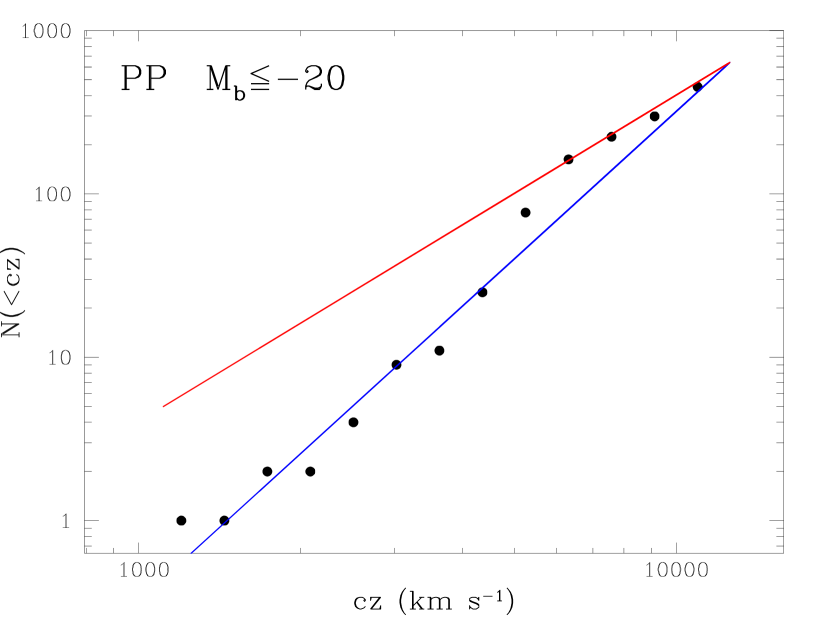
Figure 2: Number of galaxies within volumes of increasing radius in the volume–limited ($M\leq-20$) subsample of the Perseus–Pisces redshift survey of Figure  1 (filled circles). For comparison, the red line gives the relation expected for a fractal distribution with $D=2$, while the blue line refers to a homogeneous model. Apparently, the observed counts seem to stabilize around the fractal curve at large radii. (This being a cumulative distribution, points are not independent and error bars would have no meaning. See Figure 3 for an indication of the true amount of fluctuation around the differential histogram).

Let us consider the differential redshift distribution of the galaxies for the same sample, shown in Figure 3. The solid histogram in the left panel clearly shows the preponderancy of the Perseus–Pisces supercluster at $cz\sim 5500\,{\rm km\,s^{-1}}$, while again the two curves in colour show the expectation values of the counts in the $D=2$ and homogeneous cases. One can notice that the boost observed in the integral counts of Figure 2 starts where the strong positive contribution of the supercluster enters the sampled volume. The right panel shows the ratio between the observed counts and those predicted in the two scenarios, (the curve whose mean trend is closer to 1 will be the one which better describes the data). The red line (fractal case), shows a monotonic increase with scale, indicating that it predicts on the average less objects at larger and larger radii than are actually observed. The homogeneous model describes the data better, fluctuating around a substantially flat mean, although the differences between the two models for $cz>4000\,{\rm km\,s^{-1}}$ are very small and not significant. Intrinsic fluctuations due to clustering are still very strong on samples this size, and also when averaged over the large solid angle of the PP survey ($\sim 1\,sr$), they are much stronger than the Poissonian fluctuations within the bins (indicated by the error bars). Comparing the integral and differential histograms, one should probably conclude that samples of this depth are simply not large enough for using $N(r)$ as a discriminator of the global geometry.

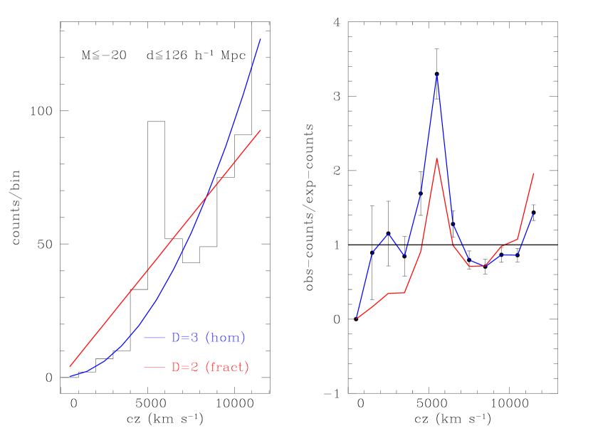
Figure 3: Histogram of the galaxy distribution as a function of distance from the observer (left panel) for the PP survey subsample. As in the previous figure, the red and blue lines give the expected behaviour for a $D=2$ fractal and a homogeneous distribution, respectively. In the right panel, the observed differential counts have been normalized to those expected for the two models. The strong positive fluctuation around $cz\simeq 5500\,{\rm km\,s^{-1}}$ corresponds to the Perseus–Pisces supercluster.

Let us therefore consider again what are presently the state–of–the–art for redshift surveys, and in particular the ESP. This redshift survey has an apparent magnitude limit of $b_{j}=19.4$ and contains radial velocities for 3342 galaxies, whose distribution in space is shown in Figure 4. Note for comparison how the largest structures in this survey are much smaller than the survey size (what R. Kirshner called “the end of greatness” when describing the similar LCRS), unlike the PP and CfA2 surveys. Based on the analysis of a preliminary version of this survey, Pietronero and collaborators again claim that the behaviour of $N(r)$ is consistent with a $D=2$ fractal. I have repeated the same exercise with the whole survey (now completed, Vettolani et al.  1997), extracting a volume–limited sample with $M\leq-20$ and $z\leq 0.189$, containing a total of 517 galaxies. One word of caution is important here: this survey is deep enough so that galaxy magnitudes have to be K–corrected before the true rest–frame absolute magnitude can be recovered (see Zucca et al.  1997 for details on the K–correction procedure). Apparently, this seems to have been neglected in the analysis presented, e.g., in P97 [see Scaramella et al.  (1997) for a more detailed investigation of this point, together with a comparison of the $N(r)$ of Abell clusters]. In Figure 5 I have plotted the integral counts $N(z)$ obtained for the ESP subsample, compared again to the expectations of the $D=2$ and $D=3$ cases, as in Figure 2.

Figure 4: Galaxy distribution in the ESO Slice Project (ESP) redshift survey.

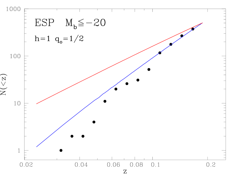
Figure 5: Number of galaxies within volumes of increasing radius in a volume–limited ($b_{J}\leq-20$) subsample of the ESP redshift survey (filled circles). The red line gives the relation expected for a fractal distribution with $D=2$, while the blue line refers to a homogeneous model. Unlike for the PP survey, and in contrast with the claims by Pietronero et al. , the observed counts on large enough scales seem to stabilize around the homogeneous model.

The counts are now performed in the full cosmological framework, assuming a spatially flat universe with $\Omega=1$, as indicated in the figure. The fractal (red) curve is computed by assuming that comoving distances are distributed according to the fractal law, and then calculating the corresponding redshift in the chosen world model. I note, however, that there is an internal inconsistency in this procedure, since the Friedmann–Robertson–Walker cosmology assumes a priori homogeneity on large scales. Therefore, we would not even be allowed to make this comparison on scales where the global cosmology starts to be important, if the fractal hypothesis were true. In other words, one would have first to re–found a different cosmology, based on a different sort of Cosmological Principle compatible with the fractal hypothesis, construct the proper distance relations, and then finally compare predictions with the observations. For our purposes, cosmological corrections are still small on these scales so that the simple FRW comparison should be meaningful.

As one can note from the figure, the integral counts seem to be very well in agreement with those expected for a homogeneous Universe on large scales. Note the low values of the counts at small radii. This is due first of all to the small survey volume within these distances (the ESP survey area is only $1^{\circ}$ thick in declination), so that bright objects are lost due to shot noise, that cuts off the bright tail of the luminosity function. (This is the same as saying that the volume is not large enough as to make the integral of the luminosity function over that volume larger than 1: since we cannot observe, say, 1/5 or 1/2 of a galaxy, no galaxy – at that luminosity – is observed). The second effect is a true underdensity in the mean distribution of galaxies in the South Galactic Pole region which seems to extend out to $\sim 140\rm\,h^{-1}\,Mpc$. This underdensity has been shown by Zucca et al.  (1997) to be the origin of the observed deficit of “bright” galaxies in the number counts.

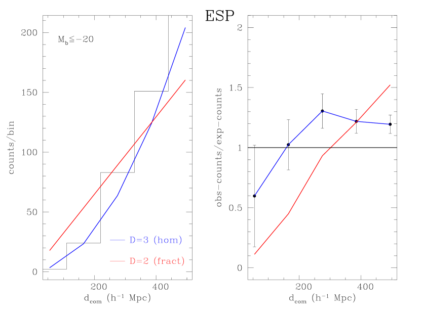
Figure 6: Differential redshift distribution for the ESP survey volume–limited subsample. The plotted points and curves in the two panels are as in figure 3.

The important result in Figure 5 is that the counts clearly stabilize around the homogeneous curve for $z>0.1$. This is in contradiction with what has been claimed by Pietronero and collaborators from the analysis of the same survey. The only explanation of the discrepancy I can find is possibly in them having improperly analysed a preliminary, incomplete version of the survey and most importantly not having performed any K–correction.

In Figure 6, just as a further indication, I show the behaviour of the differential redshift distribution for the same sample. Again, the $D=2$ fractal model (red line), overestimates the expected distribution at small distances while underestimating it at large distances.

5 So the Universe is not Fractal?

So far we have concentrated on two specific observational tests that I considered as crucial, and that explicitly show the difficulty of describing the distribution of galaxies as a pure unlimited fractal. To shortly summarize the conclusions reached so far: 1) the mean density and hence the correlation length does not depend on the sample size for the largest statistically complete redshift samples available today, and on the contrary $r_{\circ}$ is remarkably stable among surveys of very different geometry. 2) The growth of the number of galaxies in volumes of increasing radius is more consistent, within sufficiently large volumes, with a homogeneous distribution than with a fractal.

Having established this, however, what can be said about the fractal properties of the galaxy distribution in the range where galaxies are clustered, and in which their distribution shows a clear self–similar character? The classical arguments in this respect are discussed in detail in Peebles (1980; 1993), and in Mandelbrot (1982). The essence of this is that galaxy clustering on scales smaller than $\sim 5\rm\,h^{-1}\,Mpc$ is well described by a power–law correlation function $\xi(r)=(r/r_{\circ})^{-\gamma}$ with $\gamma\simeq 1.8$. On these scales $\xi(r)\gg 1$, and we have seen in § 3.1 how this implies a fractal behaviour characterized by a fractal dimension $D=3-\gamma=1.2$. N–body simulations (e.g. Valdarnini, Borgani & Provenzale 1992), statistical (Peebles 1980), and thermodynamical arguments (Saslaw 1984), seem to agree in indicating that a $\sim r^{-2}$ power–law correlation function is a sort of equilibrium attractor of fully nonlinear gravitational evolution. Independently on the way we describe it, therefore, this regime seems to be undoubtedly the product of the scale–free action of gravity.

We have also seen that, in general, a fractal regime is strictly evidenced by a power–law behaviour of $N(r)$, $\Gamma(r)$ or, better, $1+\xi(r)$. If therefore, clustering has some sort of fractal behaviour also in the linear regime (where $\xi(r)\sim 1$ or smaller), one will be capable to detect it only by looking at these functions.

Motivated by these arguments, discussed in Pietronero (1987), some years ago Guzzo et al.  (1991, G91 hereafter) studied the behaviour of $1+\xi(r)$ in the PP and CfA1 redshift surveys. The result was that consistently in both surveys this function is characterized by two distinct power–law ranges: a small–scale part with $D=1.2$ for $r<3.5\rm\,h^{-1}\,Mpc$, and a second range, between 3.5 and $\sim 20-30\rm\,h^{-1}\,Mpc$, where $1+\xi(r)$ is still well described by a power law, but with a fractal dimension $D\simeq 2.2$. They speculated that the two ranges could be evidence for two distinct physical regimes: (1) fully nonlinear gravitational clustering on small scales, and (2) quasi–linear fluctuations on larger scales, characterized by a shallower clustering, possibly still reminiscent of initial conditions. The interest in this latter range was clearly motivated by the attractive possibility to relate it directly to the linear shape of the power spectrum of density fluctuations $P(k)$. The observed behaviour implied a rather steep $P(k)$ on these scales, with $n=-D\sim-2.2$, significantly steeper than, e.g., that expected from a standard Cold Dark Matter (CDM) fluctuation spectrum on the same scales, that has an effective index close to $n=-1$. Branchini et al.  (1994) showed how a phenomenological linear power spectrum with such a slope could be numerically evolved to develop the correct small–scale $D=1.2$ slope, while providing at the same time a good match to the observed large–scale shallower clustering.

The result by G91 was certainly approximate in many respects, in particular in the treatment of redshift–space distortions. The two regimes can indeed be clearly seen only in real space: redshift–space damping produced by cluster velocity dispersions below $2-3\rm\,h^{-1}\,Mpc$ has the perverse effect of flattening down the correlation function, bringing the observed $D$ to a value around 1.6–1.8, so that when one plots $1+\xi(s)$, this is very well described by a single power law with slope $D-3\sim-1$ on all scales out to $20-30\rm\,h^{-1}\,Mpc$. For this reason, the best test of the G91 findings is provided by the distortion–free clustering measures computed from angular surveys like the APM. Qualitatively, one could already notice that the angular correlation function $w(\theta)$ from the APM survey (Maddox et al.  1990), shows a “shoulder” above $1^{\circ}$ ($\sim 4\rm\,h^{-1}\,Mpc$ at the depth of the Lick catalogue, to which that result is scaled), the same feature that G91 showed to be the fingerprint of the large–scale shallower scaling (see also Calzetti et al. 1992 for a similar inference from earlier angular data). This indication was made more explicit by the estimate of the APM real–space power spectrum, that Baugh & Efstathiou (1993), computed by de–projecting $w(\theta)$. I have replotted their estimate in Figure 7.

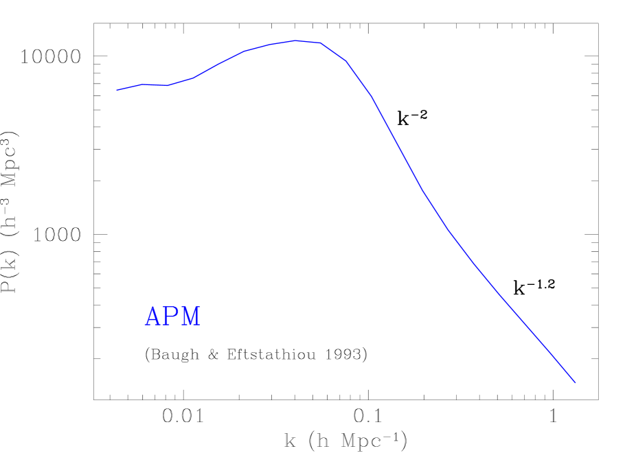
Figure 7: The real–space power spectrum measured from the APM galaxy survey. Note the two power–law regimes for $k>0.08$ h Mpc^-1, that correspond in Fourier space to the two similar scaling ranges observed in $1+\xi(r)$. Note how the logarithmic slope $n$ of the power spectrum is directly related to the fractal correlation dimension $D=-n$ in the corresponding range of scales. Error bars are omitted for clarity (see Baugh & Efstathiou 1993).

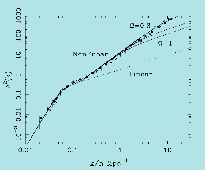
Figure 8: Observed power spectra from the APM (filled circles), and IRAS–QDOT (open circles) surveys, from Peacock (1997). The dotted line is the phenomenological model for the linear $P(k)$ that best reproduces the observed data, characterized by a power–law index above 0.08 h Mpc^-1 $n\sim-2.2$. Power spectra are here plotted as the logarithmic contribution to the variance, $\Delta^{2}(k)={\rm d}\sigma^{2}/{\rm d}\ln{k}\propto k^{3}P(k)$. [Reproduced with permission from the MNRAS].

The figure shows that at wavenumbers larger than the peak around 0.05 h Mpc^-1 the spectrum is characterized by two slopes: $k^{-2}$ at intermediate wavenumbers, and $k^{-1.2}$ at larger $k$’s (small spatial scales). These correspond, in Fourier space, to the two clustering ranges observed by G91 on $1+\xi(r)$. The transition between the two regimes is around $k\simeq 0.2$ h Mpc^-1, corresponding to the $r\sim 3-4\rm\,h^{-1}\,Mpc$ change of slope observed in the correlation function [$r\sim\lambda/4=\pi/(2k)$]. This scale, therefore, seems to assume a particularly important dynamical meaning in the clustering properties of our Universe at the present epoch: it is the typical scale below which today fluctuations are fully nonlinear.

The relation of the two power–law ranges to the linear and nonlinear regimes of evolution of the power spectrum, has been recently confirmed through a detailed investigation by Peacock (1997). Branchini et al.  (1994) simply assumed that the large–scale $D\simeq 2.2$ power law was strictly describing the behaviour of linear fluctuations, and extrapolated this regime to smaller scales to construct their phenomenological linear power spectrum. Peacock (1997), on the other hand, applies a modified version of Hamilton et al.  (1991) analytical reconstruction algorithm to the Baugh & Efstathiou APM power spectrum and to a similar real–space estimate from the IRAS–QDOT survey (Saunders et al.  1992), to obtain the linear power spectrum from the nonlinear data. The observations [expressed as variance per logarithm of $k$, $\Delta^{2}(k)\propto k^{3}P(k)$], and the reconstructed linear power spectrum (dotted line), are shown in Figure 8. The important result is that the reconstructed linear power spectrum turns out to be characterized by a an index around $n=-2.2$ for scales smaller than the turnover at $k\sim 0.08$ h Mpc^-1, as deduced by G91 and Branchini et al.  (1994) using the shape of $1+\xi(r)$.

6 Discussion and Conclusions

The main conclusions that I have reached in this harangue in defense of a homogeneous Universe can be summarized as follows.

1) There is strong evidence from the large–scale distribution of galaxies that the observed clustering does not continue to arbitrarily large scales, but is limited by a turnover to homogeneity. This cutoff scale, that we can associate to a maximum in the power spectrum $P(k)$, is most probably located around a 3D wavelength scale comprised between 100 and $200\rm\,h^{-1}\,Mpc$ and becomes evident when we properly analyze the largest surveys presently available. It is clear that even these samples have just reached this scale, and certainly we are not yet sampling well enough the largest clustering wavelengths in the galaxy density field. However, the stability of the galaxy–galaxy correlation length and the law of growth of the number of objects within larger and larger volumes are in contraddiction with a pure fractal with a well–defined $D$ on all observed scales.

2) On the other hand, within the range where they are clustered galaxies do cluster in a fractal–like way. More specifically, there is strong evidence that we are witnessing the effect of two processes, both producing a scale–free behaviour in the galaxy distribution within their respective ranges of action. At separations smaller than $\sim 3.5\rm\,h^{-1}\,Mpc$ we observe a distribution with $D=1.2$, resulting from the nonlinear gravitational evolution of the initial spectrum. On larger scales, there is a second range extending to separations of $20-30\rm\,h^{-1}\,Mpc$ in which a fractal–like scaling is also observed, but with a shallower scaling law characterized by $D=2-2.3$. We have seen that there are very good reasons to interpret this range as being directly related to initial conditions, corresponding to a linear power spectrum with a slope $n$ between $-2$ and $-2.3$. In the framework of CDM models, open models with $\Omega\simeq 0.3$ best reproduce the observed shape on small and large scales (Peacock 1997). However, the best match to the observations in absolute terms is provided by phenomenological shapes in which the maximum of $P(k)$ is much sharper than in any CDM variant (Branchini et al.  1994; Peacock 1997).

If this primordial scaling really corresponds to a fractal behaviour (to this end it would be important a better understanding of the present phase distribution of the large–scale density field as traced by galaxies, see e.g. Ghigna et al.  1994), then one can speculate how this could have developed strarting from the natural assumption of an initially gaussian density field. If initial conditions were gaussian (and therefore intrinsically non–fractal), characterized by a power–law $P(k)$ with $n\sim-2.2$ over comoving wavelengths between $\sim 1-100\rm\,h^{-1}\,Mpc$ and random phases, one could think of linear gravitational clustering (perhaps in combination with galaxy formation processes that favour the density field above a certain threshold – see e.g. Szalay & Schramm 1985), as a process that very quickly rearranges the phases of the density field, while the power spectrum slowly grows self–similarly in amplitude. This would provide the necessary phase ordering which is a key for producing fractal distributions, characterized by strongly non–random phases. In a different perspective, this stage of evolution could be seen as the build up of pancakes, i.e. the early linear growth of long–wavelength fluctuations along one preferred direction, giving rise to flattened, sheet–like structures (an interpretation already proposed by Dekel & Aarseth 1984). In fact, Provenzale et al.  (1994) explicitly showed that the observed two regimes of clustering can be reproduced also in a toy model in which: (1) galaxies are distributed as a 2D fractal on the surfaces of planar structures; (2) these are in turn randomly oriented in space in a 3D network, with a specific mean inter–plane distance. In this picture, the large–scale $D\simeq 2$ dimension would be topological, rather than fractal.

While large scales grow linearly, at the same time on small scales nonlinear gravitational clustering starts building up vigorously a different, more packed structure with $D\sim 1.2$, that grows up in time extending to larger and larger scales. Is this a true fractal distribution? It has recently been shown explicitly that the observed scaling law can be produced by a distribution of density singularities (i.e. clusters) with a certain profile (Murante et al.  1997). The observed $D=1.2$ at small separations would directly descend in this picture from the mean density profile of these clusters, that dominate two–point statistics on small scales.

My feeling is that probably on large scales (the $D\sim 2$ regime), we are seeing a true fractal essentially produced both by the re–ordering of phases along large–scale density fluctuations and the effects of galaxy formation that bias the luminous objects towards the large–scale density peaks. The result of these early processes is to form the tridimensional network of objects with scale–free clustering properties, that we observe today on scales between 5 and $\sim 50\rm\,h^{-1}\,Mpc$. On small scales, on the other hand, I find the singularity picture more realistic. In fact, nonlinear collapse (strongly anisotropic in the beginning, as driven by the initial long–wavelength distribution, i.e. preferentially along the “phase channels” provided by the large–scale structure), produces a “phase–scrambling”, with a total erasing of the initial information. The result of this process, after subsequent re–expansion, is a virialized, relaxed structure that we call a cluster, with a well–defined and rather isotropic density profile that plays the major role in producing the observed small–scale $D=1.2$ slope in the two–point correlation function. Given that we indeed observe these relaxed objects and that galaxies in clusters dominate two–point statistics on small scales, this “distribution of density singularities”, as discussed by Murante et al.  (1997), might seem a better description of the observed statistical behaviour, than that of a homogeneous fractal with the same two–point function.

At the end of the 1996 “Critical Dialogues” meeting, L. Pietronero and M. Davis agreed to wager a case of good wine (Californian vs. Italian, respectively), about which value for the galaxy correlation length will be measured by the Sloan Digital Sky Survey. The discussion I have presented here seems to point in the direction of more Italian wine to be exported to California, rather than the opposite. While we wait for the SDSS to produce its first estimate of $r_{\circ}$, however, we seem already able to draw some conclusions of methodological character. The morale of the present discussion could be that, like good wine, if fractal techniques and methods are “taken with moderation” they provide a useful perspective from which to interpret the nature and evolution of large–scale structure. This perspective is not at all in contraddiction with the classical gravitational instability description, given that an homogeneity turnover does seem to be there. This means that, unlike for a pure fractal, a mean density of the Universe can be defined and in turn the whole concept of density fluctuations makes sense. On the contrary, we have seen that statistical descriptions that are common place in the study of fractal phenomena (see e.g. Borgani 1995 for an overview), and that are often very simple (but significant) modifications of those usually applied in cosmology, can help in evidencing very important characteristics of galaxy clustering. In particular, to show where and with which properties galaxies do display a scale–free behaviour of some sort.

Continuing with the same oenological analogy, I should conclude at this point that also a good vintage wine can, if used immoderately, lead to rather annoying consequences. In the same way, I hope to have shown that the beauty and elegance of the fractal description has to be applied to the real data keeping in mind the physics of structure formation, and most importantly the whole range of subtle selection biases that affect the observations.

Acknowledgments

I am indebted to Jim Peebles for his contribution to the birth of this paper, and for his encouraging comments on the manuscript. I thank Antonello Provenzale for many stimulating discussions on this subject during the past years, and Guido Chincarini, Marc Davis, Roberto Scaramella, Gianni Zamorani, Elena Zucca, and especially Peter Schücker for very useful comments and discussions. I am grateful to all the ESP survey team for allowing me to discuss some results from the project in advance of publication, and to Carlton Baugh for providing the APM power spectrum in electronic form. John Peacock is gratefully acknowledeged for his patience in our e-mail discussions on the evolution of clustering. I would also like to acknowledge vigorous discussions with my opponents in this very stimulating controversy, Francesco Sylos–Labini and Luciano Pietronero.

Appendix A Appendix: Practical Estimators of $\xi(r)$

In P97 and in many previous works by the same authors, a basic methodological cricitism is made of the standard technique normally used to estimate $\xi(r)$ from redshift surveys in the presence of sample boundaries (e.g. Davis & Peebles 1983). The effect of the finite survey volume is usually taken into account by normalizing the observed number of pairs at each separation to that obtained from a set of random points distributed within the same volume of the survey. Without entering into the technical details of the problem, here I would only like to mention the results of two simple direct tests of the limits of this technique. To this end, Provenzale et al.   (1994) constructed simulated fractal distributions using the $\beta$–model algorithm, from which they extracted artificial mock surveys with classical “cone–like” shapes. The result was that they were not able to reproduce the observed flattening of $1+\xi(r)$ at $r>50\rm\,h^{-1}\,Mpc$ [i.e. a break in $\xi(r)$], from a pure unlimited fractal model ”observed” as the real surveys. The observed behaviour was reproduced only by a $\beta$–model with an upper cutoff to homogeneity above cubes of $\sim 50\rm\,h^{-1}\,Mpc$ side, corresponding to fluctuations with wavelength around $100\rm\,h^{-1}\,Mpc$.

The same conclusions had been reached independently by Lemson & Sanders (1991), who instead used Voronoi tesselation and Lévy flights to produce synthetic fractals by which to test the estimators of the two–point correlation function.

References

- [1] Bartlett, J., et al. (the ESP team), 1997, in preparation
- [2] Baugh, C.M., & Efstathiou, G.P., 1993, MNRAS, 265, 145
- [3] Borgani, S., 1995, Phys. Rep., 251, 1
- [4] Branchini, E., Guzzo, L. & Valdarnini, R., 1994, ApJ, 424, L5
- [5] Calzetti, D., Giavalisco, M., & Meiksin, A., 1992, ApJ, 398, 429
- [6] Castagnoli, C., & Provenzale, A., 1991, A&A, 246, 634
- [7] Charlier, C.V.L., 1908, Archiv. för Mat. Astron. Fys., 4, 1
- [8] Coleman, P.H., Pietronero, L., & Sanders, R.H., 1988, A&A, 200, L32
- [9] Davis, M., 1997, preprint, astro-ph/9610149
- [10] Davis, M., Meiksin, A., Strauss, M.A., da Costa, L.N., & Yahil, A., 1988, ApJ, 333, L9
- [11] Dekel, A., & Aarseth, S.J., 1984, ApJ, 283, 1
- [12] Di Nella, H., Montuori, M., Paturel, G., Pietronero, L., Sylos Labini, F., A&A, in press (astro-ph/9603015)
- [13] Einasto, J., Klypin, A., Saar, E., 1986, MNRAS, 219, 457
- [14] Einasto, J., et al. 1997, Nature, 385, 139
- [15] Ellis, R.S., 1997, ARA&A, in press
- [16] Fisher, K.B., Davis, M., Strauss, M.A., Yahil, A., & Huchra, J.P., 1994, MNRAS, 267, 927
- [17] Geller, M.J., & Huchra, J., 1989, Science, 246, 897
- [18] Ghigna, S., Borgani, S., Bonometto, S.A., Guzzo, L. Klypin, A., Primack, J.R., Giovanelli, R., & Haynes, M.P., 1994, ApJ, 437, L71
- [19] Giovanelli, R., & Haynes, M.P., 1991, ARA&A, 29, 499
- [20] Guzzo, L., Iovino, A., Chincarini, G., Giovanelli, R., & Haynes, M.P., 1991, ApJ, 382, L5 (G91)
- [21] Guzzo, L., Strauss, M.A., Fisher, K.B., Giovanelli, R., & Haynes, M.P., 1997, ApJ, 489, in press (astro-ph/9706150)
- [22] Hamilton, A.J.S., Kumar, P., Lu, E., & Matthews, A., 1991, ApJ, 374, L1
- [23] Iovino, A., Giovanelli, R., Haynes, M.P., Chincarini, G., & Guzzo, L. 1993, MNRAS, 265, 21
- [24] Lemson, G., & Sanders, R.H.,1991, MNRAS, 252, 319
- [25] Lin, H., 1995, PhD Thesis, University of Harvard.
- [26] Loveday, J., Maddox, S.J., Efstathiou, G., & Peterson, B.A., 1995, ApJ, 442, 457
- [27] Maddox, S.J., Efstathiou, G., Sutherland, W. J. & Loveday, J., 1990, MNRAS, 242, 43p
- [28] Mandelbrot, B.B., 1982, The Fractal Geometry of Nature (San Francisco: Freeman)
- [29] Murante, G., Provenzale, A., Spiegel, E.A., & Thierberger, R., preprint, astro-ph/9704188
- [30] Paturel, G., et al. 1995, in Information and On–Line Data in Astronomy, D. Egret & M. Albrecht eds., Kluwer, p. 115.
- [31] Peacock, J.A., 1997, MNRAS, 284, 885.
- [32] Peebles, P.J.E., 1980, The Large–Scale Structure of the Universe, (Princeton: Princeton University Press)
- [33] Peebles, P.J.E., 1993, Principles of Physical Cosmology, (Princeton: Princeton University Press)
- [34] Pietronero, L., 1987, Physica, 144A, 257
- [35] Pietronero, L., Montuori, M., & Sylos–Labini, F., 1997, preprint, astro-ph/9611197 (P97)
- [36] Provenzale, A., 1991, in Applying Fractals in Astronomy, A. Heck & J. Perdang eds., (Berlin: Springer)
- [37] Provenzale, A., Guzzo, L., & Murante, G., 1994, MNRAS, 266, 555
- [38] Saslaw, W.C., 1984, Gravitational Physics of Stellar and Galactic Systems, (Cambridge: Cambridge University Press)
- [39] Saunders, W., Rowan–Robinson, M., Lawrence, A., 1992, MNRAS, 258, 134
- [40] Scaramella, R., et al. (the ESP team), 1997, in preparation.
- [41] Szalay,A.S., & Schramm, D.N., 1985, Nature, 314, 718
- [42] Valdarnini, R., Borgani, S., & Provenzale, A., 1992, ApJ, 394, 422
- [43] Vettolani, P., et al. (the ESP team), 1997, A&A, 325, 954
- [44] Weinberg, S., 1972, Gravitation and Cosmology, (New York: Wiley)
- [45] Zucca, E., et al. (the ESP team), 1997, A&A, 326, 477