Transients from Initial Conditions: A Perturbative Analysis

Abstract

The standard procedure to generate initial conditions in numerical simulations of structure formation is to use the Zel’dovich approximation (ZA). Although the ZA correctly reproduces the linear growing modes of density and velocity perturbations, non-linear growth is inaccurately represented, particularly for velocity perturbations because of the ZA failure to conserve momentum. This implies that it takes time for the actual dynamics to establish the correct statistical properties of density and velocity fields.

We extend the standard formulation of non-linear perturbation theory (PT) to include transients as non-linear excitations of decaying modes caused by the initial conditions. These new non-linear solutions interpolate between the initial conditions and the late-time solutions given by the exact non-linear dynamics. To quantify the magnitude of transients, we focus on higher-order statistics of the density contrast $\delta$ and velocity divergence $\Theta$, characterized by the $S_{p}$ and $T_{p}$ parameters. These describe the non-Gaussianity of the probability distribution through its connected moments $\mathop{\langle}\delta^{p}\mathop{\rangle_{c}}\equiv S_{p}\mathop{\langle}\delta^{2}\mathop{\rangle}^{p-1}$, $\mathop{\langle}\Theta^{p}\mathop{\rangle_{c}}\equiv T_{p}\mathop{\langle}\Theta^{2}\mathop{\rangle}^{p-1}$. We calculate $S_{p}(a)$ and $T_{p}(a)$ to leading-order in PT with top-hat smoothing as a function of scale factor $a$.

We find that the time-scale of transients is determined, at a given order $p$, by the effective spectral index $n_{\rm eff}$. The skewness factor $S_{3}$ ($T_{3}$) attains 10$\%$ accuracy only after $a\approx 6$ ($a\approx 15$) for $n_{\rm eff}\approx 0$, whereas higher (lower) $n_{\rm eff}$ demands more (less) expansion away from the initial conditions. These requirements become much more stringent as $p$ increases, always showing slower decay of transients for $T_{p}$ than $S_{p}$. For models with density parameter $\Omega\neq 1$, the conditions above apply to the linear growth factor, thus an $\Omega=0.3$ open model requires roughly a factor of two larger expansion than a critical density model to reduce transients by the same amount. The predicted transients in $S_{p}$ are in good agreement with numerical simulations.

More accurate initial conditions can be achieved by using second-order Lagrangian PT (2LPT), which reproduces growing modes up to second-order and thus eliminates transients in the skewness parameters. We show that for $p>3$ this scheme can reduce the required expansion by more than an order of magnitude compared to the ZA. Setting up 2LPT initial conditions only requires minimal, inexpensive changes to ZA codes. We suggest simple steps for its implementation.

CITA-97-42

1 Introduction

Gravitational instability is widely considered responsible for the formation and evolution of large-scale structures in the Universe. The non-linear nature of gravitational clustering makes analytical calculations only possible for models with restrictive symmetries or in cases where the density fluctuations are small enough that a perturbative approach is possible. For this reason, numerical simulations are a vital resource for understanding how large-scale structures form and evolve in the Universe.

The standard procedure in numerical simulations is to set up the initial perturbations, assumed to be Gaussian, by using the Zel’dovich (1970) approximation (Klypin & Shandarin 1983; see also Efstathiou et al. 1985, hereafter EDFW). This gives a useful prescription to perturb the positions of particles from some regular pattern (commonly a grid or a “glass”) and assign them velocities according to the growing mode in linear perturbation theory. In this way, one can generate fluctuations with any desired power spectrum and then numerically evolve them forward in time to the present epoch.

Although the Zel’dovich approximation (hereafter ZA) correctly reproduces the linear growing modes of density and velocity perturbations, non-linear correlations are known to be inaccurate when compared to the exact dynamics (Grinstein & Wise 1987, Juszkiewicz, Bouchet & Colombi 1993, Bernardeau 1994, Catelan & Moscardini 1994, Juszkiewicz et al. 1995). This implies that it may take a non-negligible amount of time for the exact dynamics to establish the correct statistical properties of density and velocity fields. This transient behavior affects in greater extent statistical quantities which are sensitive to phase correlations of density and velocity fields; by contrast, the two-point function, variance, and power spectrum of density fluctuations at large scales can be described by linear perturbation theory, and are thus unaffected by the incorrect higher-order correlations imposed by the initial conditions.

In this work, we therefore concentrate on higher-order statistics such as the one-point cumulants of density and velocity divergence fields, characterized by the so-called $S_{p}$ and $T_{p}$ parameters (Goroff et al. 1986; see Eq. (27) below for their definition). We use non-linear perturbation theory (PT) in order to provide a quantitative description of transients. For this purpose, we extend the standard formulation of PT to include the full time-dependence of density and velocity solutions to arbitrary non-linear order in the perturbation expansion. We show that initial conditions can be thought as exciting non-linear decaying modes in the evolution of perturbations which lead to transient behavior. Although we assume the initial conditions given by the ZA, the present formalism can be useful to explore other non-Gaussian initial conditions as well. We present results up to $p=8$, although the techniques developed in this work make calculations possible to higher orders if desired with minimal extra effort. Given that current angular surveys are able to measure up to $S_{9}$ (Gaztañaga 1994; Szapudi, Meiksin & Nichol 1996), and that the situation in redshift surveys will greatly improve in the near future, it is important to address the issue of what requirements are needed in order to determine accurately these statistical measures of clustering in numerical simulations.

The problem of transients from ZA initial conditions is well known in the PT literature, and it has been pointed out many times before (e.g., Juszkiewicz, Bouchet & Colombi 1993, Juszkiewicz et al. 1995). However, the only quantitative understanding of the magnitude of this problem so far comes from the numerical work of Baugh, Gaztañaga & Efstathiou (1995, BGE hereafter), who studied the transients in the skewness of the density field and found that for CDM simulations, an expansion $a\approx 3$ away from the initial conditions was necessary to erase the memory of the ZA-induced skewness. Recently, the effect of transients in $S_{3}$ at large scales was seen in the numerical renormalization solution by Couchman & Peebles (1997, Figure 12), where fluctuations at large scales are applied by the ZA at each renormalization step and then expanded by a factor of two in scale factor. For higher order moments and velocity fields moments, there is no analysis (numerical or otherwise) available in the literature. In this sense, this work constitutes a natural development of the subject and should be useful in designing numerical simulations of cosmological structure formation.

We now give a somewhat detailed summary of the contents of this paper for those readers not familiar with the technical machinery of non-linear PT and mostly interested in the relevance of the results for numerical simulations.

In Section 2.1 we review the standard formulation of non-linear PT. Eqs. (9)-(11) show how to obtain non-linear solutions to the equations of motion by a recursive procedure from linear PT solutions, as first derived by Goroff et al. (1986).

Section 2.2 presents the description of ZA initial conditions in terms of Lagrangian trajectories (as used to set initial conditions in numerical simulations, Eqs. (12)-(13)) and in Eulerian space (Eqs. (14)-(16)), which is in fact the most convenient way to calculate the statistical properties of initial conditions. We explore two different ways of setting initial velocities, the standard ZA approach which leads to Eq. (17), and the EDFW scheme which yields Eq. (18) for the divergence of the initial peculiar velocities.

In Section 2.3, we extend the non-linear PT formalism to include a description of transients. The main result in this regard is the recursion relation in Eq. (23) which gives the non-linear solutions to the equations of motion including the properties of initial conditions (represented by the first term) and how they excite non-linear decaying modes (transients). These solutions interpolate between the initial conditions (ZA) and the late-time exact-dynamics recursion relations given by Eq. (11).

In Section 3, explicit expressions for the $S_{p}$ and $T_{p}$ are given in terms of the solutions presented in the previous section. A simple way to understand the physical meaning of the $S_{p}$ parameters is provided by the Edgeworth expansion (e.g. Juszkiewicz et al. 1995; Bernardeau & Kofman 1995) for the probability distribution function (PDF) of the standardized variable $\nu\equiv\delta/\sigma$

$$P(\nu)=P_{\rm G}(\nu)\ \Big{\{}1+\frac{1}{6}\ S_{3}\ H_{3}(\nu)\ \sigma+\Big{[}\frac{S_{4}}{24}\ H_{4}(\nu)+\frac{S_{3}^{2}}{72}\ H_{6}(\nu)\Big{]}\ \sigma^{2}+\ldots\Big{\}},$$ (1)

where $P_{\rm G}(\nu)\equiv(2\pi)^{-1/2}\ \exp(-\nu^{2}/2)$ is the Gaussian distribution, and $H_{n}(\nu)$ are the Hermite polynomials, e.g. $H_{3}(\nu)=\nu^{3}-3\nu$. An equivalent expression can be written down for the velocity divergence PDF involving the $T_{p}$ parameters. We see from Eq. (1) that as $\sigma\rightarrow 0$, the PDF approaches a Gaussian distribution. The first-order correction to Gaussianity is given by the skewness factor $S_{3}$ which, being proportional to the third moment of the PDF (see Eq. (27)), measures the asymmetry between overdense and underdense regions. Gravitational clustering leads to a positive $S_{3}$ (Peebles 1980), which means that the high-density tail of the PDF is enhanced and the underdense tail is suppressed with respect to a Gaussian distribution, as expected from the attractive nature of the gravitational force. Similarly, since underdense regions expand and occupy a larger fraction of the volume, the most probable value of $\delta$ becomes negative, from Eq. (1) the maximum of the PDF is in fact reached at

$$\delta_{{\rm max}}\approx-\frac{S_{3}}{2}\ \sigma,$$ (2)

to first order in $\sigma$. We thus see that the skewness factor $S_{3}$ contains very useful information on the shape of the PDF. Similarly, higher-order $S_{p}$ parameters provide further information on the PDF shape, for example, the next term in Eq. (1) contains a contribution from the kurtosis factor $S_{4}$ that gives the lowest-order measure of flattening of the PDF tails relative to a Gaussian distribution. Comparison with exact PDF results when available (e.g. for the ZA where the PDF can be calculated non-perturbatively, see Bernardeau & Kofman 1995) and numerical simulations (Juszkiewicz et al. 1995) shows that a few terms in Eq. (1) are good enough to reproduce the shape of the PDF near its maximum. On the other hand, the Edgeworth expansion rapidly breaks down at the tails of the distribution, even becoming non-positive definite, because they receive appreciable contributions from the whole hierarchy of $S_{p}$, and the Edgeworth series cannot be truncated at finite order. In fact, the use of powerful generating function techniques (Balian & Schaeffer 1989; Bernardeau 1992, 1994; Bernardeau & Kofman 1995), which can be thought as a resummation of the Edgeworth expansion, shows that the tails of the PDF in the asymptotic region are determined by the infinite series of $S_{p}$ parameters through their generating function.

In summary, the main point of this digression is to convince the reader of the physical relevance of the $S_{p}$ and $T_{p}$ parameters as statistical measures of clustering. It should be clear from this discussion that an accurate determination of these is desired in numerical simulations in order to represent the statistics of large-scale structures correctly (BGE; Gaztañaga & Baugh 1995; Łokas et al. 1995; Juszkiewicz et al. 1995; Colombi, Bouchet & Hernquist 1996; Bernardeau et al. 1997). Regarding the calculation of $S_{p}$ and $T_{p}$ from leading-order (tree-level) PT (that is, at lowest non-vanishing order in the variance of the density field), it turns out that vertices (defined in Eq. (32)) contain all the necessary information about the non-linear dynamics. A recursion relation for vertices that includes transients is presented in Appendix A.

In Section 4 we present the perturbative results for transients in $S_{p}$ and $T_{p}$. Figure 1 shows the magnitude of transients for $S_{p}$ ($3\leq p\leq 8$) for different spectra, and similarly for $T_{p}$ in Fig. 2. A comparison with numerical simulations with initial velocities as in EDFW is presented in Fig. 5. Figures 11 and 12 present the corresponding transients in $S_{p}$ and $T_{p}$ when initial conditions are generated using second-order Lagrangian PT (2LPT). Note the significant improvement when compared to the equivalent plots in Figs. 1 and 2 for the ZA.

Section 5 contains our conclusions and a final discussion. Technical material regarding details of the calculations and further analytic results are presented in Appendices A, B, and C. Finally, Appendix D presents a simple procedure to implement second-order Lagrangian PT initial conditions in numerical simulations which requires minimal numerically inexpensive modifications to a standard ZA code.

2 Dynamics

2.1 Standard Formulation of Perturbation Theory

In the single-stream approximation, prior to orbit crossing, one can adopt a fluid description of the cosmological $N$-body problem, where the relevant equations of motion correspond to conservation of mass and momentum and the Poisson equation (e.g., Peebles 1980). Since vorticity decays in an expanding universe, the system can be described completely in terms of the density contrast $\delta({\hbox{\BF x}})\equiv[\rho({\hbox{\BF x}},t)-\bar{\rho}]/\bar{\rho}$ and the velocity divergence, $\theta\equiv{\bf\nabla}\cdot{\hbox{\BF v}}$, where ${\hbox{\BF v}}({\hbox{\BF x}})$ is the peculiar velocity. Defining the conformal time $\tau=\int dt/a$, where $a(\tau)$ is the cosmic scale factor, and the conformal expansion rate ${\cal H}\equiv{d\ln a/{d\tau}}=Ha$, where $H$ is the Hubble constant, the equations of motion in Fourier space become (e.g. Scoccimarro & Frieman 1996)

$${\partial\tilde{\delta}({\hbox{\BF k}},\tau)\over{\partial\tau}}+\tilde{\theta}({\hbox{\BF k}},\tau)=-\int d^{3}k_{1}\int d^{3}k_{2}\ [\delta_{\rm D}]_{2}\ \alpha({\hbox{\BF k}},{\hbox{\BF k}}_{1})\ \tilde{\theta}({\hbox{\BF k}}_{1},\tau)\ \tilde{\delta}({\hbox{\BF k}}_{2},\tau),$$

$${\partial\tilde{\theta}({{\hbox{\BF k}}},\tau)\over{\partial\tau}}+{\cal H}(\tau)\ \tilde{\theta}({\hbox{\BF k}},\tau)+{3\over 2}\ \Omega\ {\cal H}^{2}(\tau)\ \tilde{\delta}({\hbox{\BF k}},\tau)=-\int d^{3}k_{1}\int d^{3}k_{2}\ [\delta_{\rm D}]_{2}\ \beta({\hbox{\BF k}},{\hbox{\BF k}}_{1},{\hbox{\BF k}}_{2})\ \tilde{\theta}({\hbox{\BF k}}_{1},\tau)\ \tilde{\theta}({\hbox{\BF k}}_{2},\tau),$$

(3b)

where we used the Fourier transform representation $\tilde{\delta}({\hbox{\BF k}})=(2\pi)^{-3}\int d^{3}x\,\delta({\hbox{\BF x}})\,e^{-i{\hbox{\BFs k}}\cdot{\hbox{\BFs x}}}$. In Eqs. (3), k denotes a comoving wave number, $[\delta_{\rm D}]_{2}\equiv\delta_{\rm D}({\hbox{\BF k}}-{\hbox{\BF k}}_{1}-{\hbox{\BF k}}_{2})$, with $\delta_{\rm D}$ the Dirac delta distribution, and

$$\alpha({\hbox{\BF k}},{\hbox{\BF k}}_{1})\equiv{{\hbox{\BF k}}\cdot{\hbox{\BF k}}_{1}\over{k_{1}^{2}}},\qquad\beta({\hbox{\BF k}},{\hbox{\BF k}}_{1},{\hbox{\BF k}}_{2})\equiv{k^{2}({\hbox{\BF k}}_{1}\cdot{\hbox{\BF k}}_{2})\over{2\ k_{1}^{2}\ k_{2}^{2}}},$$ (4)

which describe mode-coupling due to the non-linear dynamics. Equations (3) and (3b) are valid in an arbitrary homogeneous and isotropic universe, which evolves according to the standard Friedmann equations. In linear PT, the solution to the equations of motion (3) and (3b) is given by

$$\tilde{\delta}({\hbox{\BF k}},\tau) = D(\tau)\ \delta_{1}({\hbox{\BF k}}),$$ (5)

$$\tilde{\theta}({\hbox{\BF k}},\tau) = -{\cal H}(\tau)\ f(\Omega,\Lambda)\ D(\tau)\ \delta_{1}({\hbox{\BF k}}),$$ (6)

where $D(\tau)$ is linear growing mode, which from the equations of motion must satisfy

$$\frac{d^{2}D}{d\tau^{2}}+{\cal H}(\tau)\ \frac{dD}{d\tau}=\frac{3}{2}\ \Omega\ {\cal H}^{2}(\tau)\ D,$$ (7)

and $f(\Omega,\Lambda)$ is defined as

$$f(\Omega,\Lambda)\equiv\frac{d\ln D}{d\ln a}=\frac{1}{\cal H}\frac{d\ln D}{d\tau}.$$ (8)

Explicit expressions or $D(\tau)$ and $f(\Omega,\Lambda)$ are not needed for our purposes (see e.g. Peebles 1980), but useful fits in the cosmologically interesting cases are $f(\Omega,\Lambda)\approx\Omega^{3/5}$ when $\Lambda=0$ (Peebles 1976), and $f(\Omega,\Lambda)\approx\Omega^{5/9}$ when $\Omega+\Omega_{\Lambda}=1$ (Bouchet et al. 1995). When $\Omega=1$, the linear growth factor $D(\tau)$ becomes the scale factor $a(\tau)$ and $f=1$. In this case, the PT solutions at each order $n$ scale as $a^{n}(\tau)$ and a general recursion relation is available that gives the PT solutions at arbitrary order (Goroff et al. 1986, see Eqs. (11) below). When $\Omega\neq 1$ and/or $\Lambda\neq 0$, the PT solutions at each order become increasingly more complicated, due to the fact that growing modes at order $n$ in PT do not scale as $a^{n}(\tau)$. Furthermore, the solutions at each order become non-separable functions of $\tau$ and k (Bouchet et al. 1992, 1995; Bernardeau 1994b; Catelan et al. 1995), and there appear to be no general recursion relations for the PT kernels in an arbitrary FRW cosmology. However, a simple approximation to the equations of motion, $\Omega/f^{2}=1$, noted by Martel & Freudling (1991) for second order PT, leads to separable solutions to arbitrary order in PT in which the linear growth factor $D(\tau)$ plays the role of the scale factor, and the same recursion relations as in the Einstein-de Sitter case are obtained for the PT kernels (Scoccimarro et al. 1998). All the information on the dependence of the PT solutions on the cosmological parameters $\Omega$ and $\Lambda$ is then encoded in the linear growth factor, $D(\tau)$, which in turn corresponds to the normalization of the linear power spectrum. Equivalently, in this case the equations of motion can be written independently of cosmology by taking the linear growth factor as a time variable using Eq. (8) (Nusser & Colberg 1997).

The PT solutions for arbitrary cosmological models in this approximation can be written down as (Scoccimarro et al. 1998, Appendix B.3)

$$\tilde{\delta}({\hbox{\BF k}},\tau) = \sum_{n=1}^{\infty}D^{n}(\tau)\ \delta_{n}({\hbox{\BF k}}),$$ (9a)

$$\tilde{\theta}({\hbox{\BF k}},\tau) = -{\cal H}(\tau)\ f(\Omega,\Lambda)\sum_{n=1}^{\infty}D^{n}(\tau)\ \theta_{n}({\hbox{\BF k}}),$$ (9b)

The equations of motion then determine $\delta_{n}({\hbox{\BF k}})$ and $\theta_{n}({\hbox{\BF k}})$ in terms of the linear fluctuations,

$$\delta_{n}({\hbox{\BF k}}) = \int d^{3}k_{1}\ldots\int d^{3}k_{n}\ [\delta_{\rm D}]_{n}\,F_{n}^{(s)}({\hbox{\BF k}}_{1},\ldots,{\hbox{\BF k}}_{n})\ \delta_{1}({\hbox{\BF k}}_{1})\cdots\delta_{1}({\hbox{\BF k}}_{n}),$$ (10a)

$$\theta_{n}({{\hbox{\BF k}}}) = \int d^{3}k_{1}\ldots\int d^{3}k_{n}\ [\delta_{\rm D}]_{n}\,G_{n}^{(s)}({\hbox{\BF k}}_{1},\ldots,{\hbox{\BF k}}_{n})\ \delta_{1}({\hbox{\BF k}}_{1})\ldots\delta_{1}({\hbox{\BF k}}_{n}).$$ (10b)

where $[\delta_{\rm D}]_{n}\equiv[\delta_{\rm D}]({\hbox{\BF k}}-{\hbox{\BF k}}_{1}-\cdots-{\hbox{\BF k}}_{n})$, and the functions $F_{n}^{(s)}$ and $G_{n}^{(s)}$ are constructed from the fundamental mode coupling functions $\alpha({{\hbox{\BF k}}},{{\hbox{\BF k}}}_{1})$ and $\beta({{\hbox{\BF k}}},{{\hbox{\BF k}}}_{1},{{\hbox{\BF k}}}_{2})$ by a recursive procedure (Goroff et al. 1986; Jain & Bertschinger 1994),

$$F_{n}({\hbox{\BF k}}_{1},\ldots,{\hbox{\BF k}}_{n}) = \sum_{m=1}^{n-1}{G_{m}({\hbox{\BF k}}_{1},\ldots,{\hbox{\BF k}}_{m})\over{(2n+3)(n-1)}}\Bigl{[}(2n+1)\ \alpha({\hbox{\BF k}},{\hbox{\BF k}}^{(m)})\ F_{n-m}({\hbox{\BF k}}_{m+1},\ldots,{\hbox{\BF k}}_{n})$$ (11a)

$$\qquad+2\ \beta({\hbox{\BF k}},{\hbox{\BF k}}^{(m)},{\hbox{\BF k}}^{(n-m)})\ G_{n-m}({\hbox{\BF k}}_{m+1},\ldots,{\hbox{\BF k}}_{n})\Bigr{]},$$

$$G_{n}({\hbox{\BF k}}_{1},\ldots,{\hbox{\BF k}}_{n}) = \sum_{m=1}^{n-1}{G_{m}({\hbox{\BF k}}_{1},\ldots,{\hbox{\BF k}}_{m})\over{(2n+3)(n-1)}}\Bigl{[}3\ \alpha({\hbox{\BF k}},{\hbox{\BF k}}^{(m)})\ F_{n-m}({\hbox{\BF k}}_{m+1},\ldots,{\hbox{\BF k}}_{n})$$ (11b)

$$\qquad+2n\ \beta({\hbox{\BF k}},{\hbox{\BF k}}^{(m)},{\hbox{\BF k}}^{(n-m)})\ G_{n-m}({\hbox{\BF k}}_{m+1},\ldots,{\hbox{\BF k}}_{n})\Bigr{]}$$

(where ${\hbox{\BF k}}^{(m)}\equiv{\hbox{\BF k}}_{1}+\ldots+{\hbox{\BF k}}_{m}$, ${\hbox{\BF k}}^{(n-m)}\equiv{\hbox{\BF k}}_{m+1}+\ldots+{\hbox{\BF k}}_{n}$, ${\hbox{\BF k}}\equiv{\hbox{\BF k}}^{(m)}+{\hbox{\BF k}}^{(n-m)}$, and $F_{1}=G_{1}\equiv 1$). Symmetrizing $F_{n}$ and $G_{n}$ over the wavectors ${\hbox{\BF k}}_{1},\ldots,{\hbox{\BF k}}_{n}$ leads to $F_{n}^{(s)}$ and $G_{n}^{(s)}$ as needed in Eq. (10).

2.2 Initial Conditions: Zel’dovich Approximation

Let us now discuss the perturbative formulation of the Zel’dovich (1970) approximation, which we shall use to calculate the statistical properties of the initial conditions. In the ZA, the motion of each particle ${\hbox{\BF x}}({\hbox{\BF q}},\tau$) at initial position q is obtained by applying linear PT to its Lagrangian displacement, ${\bf\Psi}({\hbox{\BF q}},\tau)$,

$${\hbox{\BF x}}({\hbox{\BF q}},\tau)={\hbox{\BF q}}+{\bf\Psi}({\hbox{\BF q}},\tau)\approx{\hbox{\BF q}}-D(\tau)\ {\bf\nabla}\phi^{(1)}({\hbox{\BF q}}),$$ (12)

where $\phi^{(1)}({\hbox{\BF q}})$ denotes a Lagrangian potential given by the initial conditions, see Appendix D for a more detailed discussion of ZA in Lagrangian space. This implies that the velocities of particles initially at q are given by

$${\hbox{\BF v}}\approx-D(\tau)\ {\cal H}(\tau)\ f\ {\bf\nabla}\phi^{(1)}({\hbox{\BF q}}).$$ (13)

In Eulerian space, it can be shown that the ZA is equivalent to the dynamics obtained by replacing the Poisson equation by the ansatz (Munshi & Starobinsky 1994, Hui & Bertschinger 1996)

$${\hbox{\BF v}}({\hbox{\BF x}},\tau)=-\frac{2f}{3\Omega{\cal H}(\tau)}{\bf\nabla}\Phi({\hbox{\BF x}},\tau),$$ (14)

which is the relation between velocity ${\hbox{\BF v}}({\hbox{\BF x}},\tau)$ and gravitational potential $\Phi({\hbox{\BF x}},\tau)$ valid in linear PT theory. The ZA therefore fails to conserve momentum, i.e. the Euler equation will only be satisfied to linear order. When calculating one-point cumulants of density and velocity fields, is convenient to use the perturbative version of ZA, since the non-perturbative probability distribution function (PDF) is singular due to caustic formation in the sense that one-point cumulants $\mathop{\langle}\delta^{p}\mathop{\rangle_{c}}$ of the density field diverge for $p>1$ due to the high-density tail (e.g., see Bernardeau & Kofman 1995). The perturbative formulation of ZA follows from replacing Eq. (14) into the equations of motion (3), which yields the corresponding recursion relations (Scoccimarro & Frieman 1996)

$$F_{n}^{\rm ZA}({\hbox{\BF k}}_{1},\ldots,{\hbox{\BF k}}_{n}) = \sum_{m=1}^{n-1}{G_{m}^{\rm ZA}({\hbox{\BF k}}_{1},\ldots,{\hbox{\BF k}}_{m})\over{n(n-1)}}\Bigl{[}(n-1)\ \alpha({\hbox{\BF k}},{\hbox{\BF k}}^{(m)})\ F_{n-m}^{\rm ZA}({\hbox{\BF k}}_{m+1},\ldots,{\hbox{\BF k}}_{n})$$ (15a)

$$\qquad\qquad\qquad\qquad\qquad+\beta({\hbox{\BF k}},{\hbox{\BF k}}^{(m)},{\hbox{\BF k}}^{(n-m)})\ G_{n-m}^{\rm ZA}({\hbox{\BF k}}_{m+1},\ldots,{\hbox{\BF k}}_{n})\Bigr{]},$$

$$G_{n}^{\rm ZA}({\hbox{\BF k}}_{1},\ldots,{\hbox{\BF k}}_{n}) = \frac{1}{(n-1)}\sum_{m=1}^{n-1}G_{m}^{\rm ZA}({\hbox{\BF k}}_{1},\ldots,{\hbox{\BF k}}_{m})\ \beta({\hbox{\BF k}},{\hbox{\BF k}}^{(m)},{\hbox{\BF k}}^{(n-m)})\ G_{n-m}^{\rm ZA}({\hbox{\BF k}}_{m+1},\ldots,{\hbox{\BF k}}_{n}).$$ (15b)

Upon symmetrization these give a simple result for the density field PT kernels (Grinstein & Wise 1987)

$$F_{n}^{\rm ZA}({\hbox{\BF k}}_{1},\ldots,{\hbox{\BF k}}_{n})=\frac{1}{n!}\frac{({{\hbox{\BF k}}}\cdot{\hbox{\BF k}}_{1})}{k_{1}^{2}}\ldots\frac{({{\hbox{\BF k}}}\cdot{\hbox{\BF k}}_{n})}{k_{n}^{2}}.$$ (16)

In numerical simulations, the ZA is generally used to set the initial perturbations as follows (see e.g. EDFW). A Gaussian density field, $\delta_{\ell}({\hbox{\BF k}})$ is generated in Fourier space from the desired linear power spectrum, and therefore the Lagrangian potential $\tilde{\phi}^{(1)}({\hbox{\BF k}})=-\delta_{\ell}({\hbox{\BF k}})/k^{2}$ is Fourier transformed and its gradient taken to yield ${\bf\nabla}_{q}\phi^{(1)}({\hbox{\BF q}})$ at each “unperturbed” particle position, denoted by q, which is usually described by a grid or a “glass”. This gives the displacement field which is used in Equation (12) to displace the particles from their unperturbed positions and imposes the ZA density field from the initial Gaussian field, i.e. $\delta^{\rm ZA}({\hbox{\BF x}})={\cal M}[\delta_{\ell}({\hbox{\BF q}})]$, where ${\cal M}$ denotes the ZA mapping implied by Eqs. (10a) and (16). Equation (13) can then be used to assign the velocities to particles. In this case, the velocities then satisfy

$$\theta({\hbox{\BF x}})=-f\ {\cal H}\ \sum_{n=1}^{\infty}D^{n}(\tau)\ \int d^{3}k_{1}\ldots\int d^{3}k_{n}\ [\delta_{\rm D}]_{n}\,G_{n}^{\rm ZA}({\hbox{\BF k}}_{1},\ldots,{\hbox{\BF k}}_{n})\ \delta_{\ell}({\hbox{\BF k}}_{1})\ldots\delta_{\ell}({\hbox{\BF k}}_{n}).$$ (17)

It is in fact straightforward but tedious to show that Eq. (13) in Lagrangian space implies Eq. (17) in Eulerian space with the kernels $G_{n}^{\rm ZA}$ given by Eq. (15b).

Although most existing initial conditions codes use this prescription to set up their ZA initial conditions, there is another prescription to set initial velocities suggested by EDFW, which avoids the high initial velocities that result from Eq. (13) because of small-scale density fluctuations approaching unity when starting a simulation at late epochs (low redshift). This procedure corresponds to recalculate the velocities from the gravitational potential due to the perturbed particle positions, obtained by solving again Poisson equation after particles have been displaced according to Eq. (12). Linear PT is then applied to the density field to obtain the velocities, which implies instead of Eq. (13) and Eq. (17) that

$$\theta({\hbox{\BF x}})=-f\ {\cal H}\ \delta^{\rm ZA}({\hbox{\BF x}})=-f\ {\cal H}\ \sum_{n=1}^{\infty}D^{n}(\tau)\ \int d^{3}k_{1}\ldots\int d^{3}k_{n}\ [\delta_{\rm D}]_{n}\,F_{n}^{\rm ZA}({\hbox{\BF k}}_{1},\ldots,{\hbox{\BF k}}_{n})\ \delta_{\ell}({\hbox{\BF k}}_{1})\ldots\delta_{\ell}({\hbox{\BF k}}_{n}).$$ (18)

Therefore, in this case, the initial velocity field is such that the divergence field $\Theta(x)\equiv\theta({\hbox{\BF x}})/(-f\ {\cal H})$ has the same higher-order correlations as the ZA density perturbations. Comparing Eq. (17) and (18) we see that both prescriptions agree in linear PT, where $F_{1}^{\rm ZA}=G_{1}^{\rm ZA}=1$, but they differ at second and higher-order PT, since $F_{n}^{\rm ZA}\neq G_{n}^{\rm ZA}$ for $n>1$. This implies that these two different alternatives of setting the initial velocities affect the magnitude of the transients, as we shall see below. It turns out that in fact, the prescription given by Eq. (18) is closer to the exact dynamics given by Eqs. (10b) and (11b) than Eq. (17), therefore, the second method will excite less decaying modes and consequently transients will decay faster than in the standard ZA scheme.

2.3 Transients in Perturbation Theory

Perturbation theory describes the non-linear dynamics as a collection of linear waves, $\delta_{1}({\hbox{\BF k}})$, interacting through the mode-coupling functions $\alpha$ and $\beta$ in Eq. (4). Even if the initial conditions are set in the growing mode, after scattering due to non-linear interactions waves do not remain purely in the growing mode. In the standard treatment, presented in Section 2.1, the subdominant time-dependencies that necessarily appear due to this process have been neglected, i.e., only the fastest growing mode (proportional to $D^{n}$) is taken into account at each order $n$ in PT. In this subsection we generalize the previous results to include the full time dependence of the solutions at every order in PT. This is necessary to properly address the problem of transients from ZA initial conditions.

In this case we write the perturbative solutions as (see Eqs. (9)):

$$\tilde{\delta}({\hbox{\BF k}},\tau) = \sum_{n=1}^{\infty}D^{n}(\tau)\ \delta_{n}({\hbox{\BF k}},D),$$ (19a)

$$\tilde{\theta}({\hbox{\BF k}},\tau) \equiv -{\cal H}(\tau)\ f(\Omega,\Lambda)\ \Theta({\hbox{\BF k}},\tau)=-{\cal H}(\tau)\ f(\Omega,\Lambda)\sum_{n=1}^{\infty}D^{n}(\tau)\ \theta_{n}({\hbox{\BF k}},D),$$ (19b)

where $\delta_{n}$ and $\theta_{n}$ are written in terms of PT kernels as in Equation (10)

$$\Phi_{a}^{(n)}({\hbox{\BF k}},D)=\int d^{3}k_{1}\ldots\int d^{3}k_{n}\ [\delta_{\rm D}]_{n}\ {\cal F}_{a}^{(n)}({\hbox{\BF k}}_{1},\ldots,{\hbox{\BF k}}_{n};D)\ \delta_{1}({\hbox{\BF k}}_{1})\cdots\delta_{1}({\hbox{\BF k}}_{n}),$$ (20)

where $a=1,2$ and $\Phi_{1}^{(n)}\equiv\delta_{n}$, $\Phi_{2}^{(n)}\equiv\theta_{n}$. The kernels ${\cal F}_{a}^{(n)}$ now depend on the linear growth factor $D(\tau)$ and reduce to the ones in the previous section when transients die out, that is ${\cal F}_{1}^{(n)}\rightarrow F_{n}$, ${\cal F}_{2}^{(n)}\rightarrow G_{n}$ when $D(\tau)\rightarrow\infty$. Also, Eq. (20) incorporates in a convenient way initial conditions, if we assume that at $D=1$, ${\cal F}_{a}^{(n)}={\cal I}_{a}^{(n)}$, we effectively reduce the non-Gaussianity of initial conditions to a Gaussian problem, i.e. where the linear solutions $\delta_{1}({\hbox{\BF k}})$ are Gaussian random fields. The kernels ${\cal I}_{a}^{(n)}$ describe the initial correlations imposed at the start of the simulation, for the standard ZA scheme we have (see Eq. (17))

$${\cal I}_{1}^{(n)}=F_{n}^{\rm ZA},\ \ \ \ \ {\cal I}_{2}^{(n)}=G_{n}^{\rm ZA},$$ (21)

whereas for velocities set from perturbed particle positions we have instead (see Eq. (18))

$${\cal I}_{1}^{(n)}=F_{n}^{\rm ZA},\ \ \ \ \ {\cal I}_{2}^{(n)}=F_{n}^{\rm ZA}.$$ (22)

The recursion relations for ${\cal F}_{a}^{(n)}$, which solve the non-linear dynamics at arbitrary order in PT, can be obtained by replacing Eq. (20) into the equations of motion, which yields

$${\cal F}_{a}^{(n)}({\hbox{\BF k}}_{1},\ldots,{\hbox{\BF k}}_{n};z) = {\rm e}^{-nz}\ g_{ab}(z)\ {\cal I}_{b}^{(n)}({\hbox{\BF k}}_{1},\ldots,{\hbox{\BF k}}_{n})+\sum_{m=1}^{n-1}\int_{0}^{z}ds\ {\rm e}^{n(s-z)}\ g_{ab}(z-s)\ \gamma_{bcd}({\hbox{\BF k}},{\hbox{\BF k}}^{(m)},{\hbox{\BF k}}^{(n-m)})$$ (23)

$$\times\ {\cal F}_{c}^{(m)}({\hbox{\BF k}}_{1},\ldots,{\hbox{\BF k}}_{m};s)\ {\cal F}_{d}^{(n-m)}({\hbox{\BF k}}_{m+1},\ldots,{\hbox{\BF k}}_{n};s),$$

where $z\equiv\ln D(\tau)$ and we have assumed the summation convention over repeated indices, which run between 1 and 2. In Equation (23) the matrix

$$g_{ab}(z)=\frac{{\rm e}^{z}}{5}\Bigg{[}\begin{array}[]{rr}3&2\\ 3&2\end{array}\Bigg{]}-\frac{{\rm e}^{-3z/2}}{5}\Bigg{[}\begin{array}[]{rr}-2&2\\ 3&-3\end{array}\Bigg{]},$$ (24)

is the linear propagator (Scoccimarro 1997b). The first term represents the propagation of linear growing mode solutions, where the second corresponds to the decaying modes propagation. That is, in linear perturbation theory, density and velocity perturbations propagate in time according to

$$\Phi_{a}^{(1)}(z)=g_{ab}(z)\ \Phi_{b}^{(1)}(0).$$ (25)

If initial conditions are set in the growing mode, then $\Phi_{a}^{(1)}(0)\propto(1,1)$ vanishes upon contraction with the second term in $g_{ab}(z)$, whereas the first term reduces to the familiar $\Phi_{a}^{(1)}(z)={\rm e}^{z}\Phi_{a}^{(1)}(0)=D(\tau)\ \Phi_{a}^{(1)}(0)$. The “scattering matrix” $\gamma_{abc}$ encodes the non-linear interactions and is given by

$$\gamma_{121}({\hbox{\BF k}},{\hbox{\BF k}}_{1},{\hbox{\BF k}}_{2}) = \alpha({\hbox{\BF k}},{\hbox{\BF k}}_{1}),$$ (26a)

$$\gamma_{222}({\hbox{\BF k}},{\hbox{\BF k}}_{1},{\hbox{\BF k}}_{2}) = \beta({\hbox{\BF k}},{\hbox{\BF k}}_{1},{\hbox{\BF k}}_{2}),$$ (26b)

and zero otherwise, with ${\hbox{\BF k}}\equiv{\hbox{\BF k}}_{1}+{\hbox{\BF k}}_{2}$. Note that since $g_{ab}(z)\rightarrow\delta_{ab}$ as $z\rightarrow 0^{+}$, in Eq. (23) the kernels ${\cal F}_{a}^{(n)}$ reduce to ${\cal I}_{a}^{(n)}$ at $D=1$, where the initial conditions are set. Equation (23) reduces to the standard recursion relations in Eq. (11) for Gaussian initial conditions (${\cal I}_{a}^{(n)}=0$ for $n>1$) when transients are neglected, i.e. the time dependence of ${\cal F}_{a}^{(n)}$ is neglected and the lower limit of integration is replaced by $s=-\infty$. Also, it is easy to check from Eq. (23) that if ${\cal I}_{a}^{(n)}=(F_{n},G_{n})$, then ${\cal F}_{a}^{(n)}=(F_{n},G_{n})$, as it should be. In what follows, the kernels in Eq. (23) are assumed to be symmetrized over its arguments. Note that these kernels are no longer a separable function of wave-vectors and time.

Equation (23) gives useful insight into the nature of nonlinear PT solutions. For example, second order solutions are built from the interaction (represented by the $\gamma$ matrix) of two linear waves that are propagated freely to the present time using Eq. (24), plus the contribution from initial conditions propagated to the present represented by the first term in Eq. (23). After scatterings, waves do not remain purely in their growing modes, and from Eq. (23) one can check that there is a contribution from decaying modes propagation even for the fastest growing mode included in standard treatments of PT. More importantly for the present purposes is the fact that the contribution to the PT solutions at a given order $n$ and “time” $z$ depend on all the $n$-scattering processes that happened between $s=z$ and $s=1$, where initial conditions are set. By assuming that initial conditions are set in the “infinite past” ($s=-\infty$), the standard formulation of PT presented in the previous section contains no information on the time scale that takes to erase the memory of the correlations imposed by the initial conditions. A more detailed treatment of this formalism and other applications is left for a future paper (Scoccimarro 1997b).

3 Statistics

We are interested in one-point cumulant statistics for the density and velocity divergence fields, which can be characterized by the $S_{p}$ and $T_{p}$ parameters defined as

$$S_{p}(R)\equiv\frac{\mathop{\langle}\delta^{p}(R)\mathop{\rangle_{c}}}{\mathop{\langle}\delta^{2}(R)\mathop{\rangle}^{p-1}}\ \ \ \ \ \ \ \ \ \ T_{p}(R)\equiv\frac{\mathop{\langle}\Theta^{p}(R)\mathop{\rangle_{c}}}{\mathop{\langle}\Theta^{2}(R)\mathop{\rangle}^{p-1}},$$ (27)

where $R$ is the smoothing scale, and the subscript $c$ denotes the connected contribution, i.e. the gaussian value is subtracted off. Note that we define cumulants for the velocity divergence field in terms of $\Theta({\hbox{\BF x}})$ as defined in Eq. (19b), which differs from the standard convention by a factor $(-1)^{p}$. In this work, we use top-hat smoothing, which is described by a window function $W_{\rm TH}(kR)$

$$W_{\rm TH}(x)=\sqrt{\frac{9\pi}{2}}\ \frac{J_{3/2}(x)}{x^{3/2}}=\frac{3}{x^{3}}\ [\sin(x)-x\cos(x)]$$ (28)

in the Fourier domain, where $J_{\nu}(x)$ is a Bessel function. To simplify the notation, we henceforth denote:

$$d\sigma^{2}_{i}\equiv 4\pi\ k_{i}^{2}\ dk_{i}\ P(k_{i})\ \ \ \ \ \ \ \ \ \ W_{i\ldots j}\equiv W_{\rm TH}(|{\hbox{\BF k}}_{i}+\ldots+{\hbox{\BF k}}_{j}|R),$$ (29)

where $P(k)$ is the power spectrum, and $\sigma^{2}$ denotes the variance of the density field fluctuations

$$\mathop{\langle}\delta({\hbox{\BF k}})\delta({\hbox{\BF k}}^{\prime})\mathop{\rangle}\equiv\delta_{\rm D}({\hbox{\BF k}}+{\hbox{\BF k}}^{\prime})\ P(k)\ \ \ \ \ \ \ \ \ \ \sigma^{2}(R)\equiv\int d^{3}k\ P(k)\ W^{2}_{\rm TH}(kR).$$ (30)

A systematic framework for calculating correlations of cosmological fields in PT has been formulated using diagrammatic techniques (Fry 1984; Goroff et al. 1986; Wise 1988; Scoccimarro & Frieman 1996). From this point of view, leading order PT for the statistical quantities of interest corresponds to tree graphs, next-to-leading order PT contributions can be described in terms of one-loop graphs, etc. These diagrammatic techniques assume Gaussian initial conditions, although in principle they can be extended to any non-Gaussian model by adding the appropriate new vertices (Wise 1988). In this work we are interested in a very particular non-Gaussian initial condition, that given by the ZA as usually imposed to start numerical simulations. As shown in the previous section, in this case one can include the non-Gaussianity directly into the non-linear solutions and therefore the problem reduces effectively to one dealing with Gaussian initial conditions.

We now write down the standard expressions for the $S_{p}$ parameters in terms of non-linear kernels. In the discussion that follows, analogous analysis always applies to the velocity divergence. In the following we shall use the scale factor $a(\tau)$ to denote the time dependence, but in models with density parameter $\Omega\neq 1$ the same equations will be valid upon replacing $a(\tau)$ by the linear growth factor $D(\tau)$. For the skewness factor, we have

$$S_{3}(R,a)=\frac{6}{\sigma^{4}(R)}\int P_{1}d^{3}k_{1}\ P_{2}d^{3}k_{2}\ W_{1}W_{12}W_{2}\ {\cal F}_{1}^{(2)}({\hbox{\BF k}}_{1},{\hbox{\BF k}}_{2};a).$$ (31)

The calculation of tree-level diagrams such as this and the expressions that follow is simplified by using the fact that tree-level PT corresponds to taking the spherical average of PT kernels (Bernardeau 1992, 1994b). We therefore define the angular averaged smoothed kernels $\omega_{a}^{(n)}$ by ($a=1,2$):

$$\frac{1}{n!}\ (\nu_{n},\mu_{n})\equiv\omega_{a}^{(n)}\equiv\int\ \Big{(}\frac{d\Omega_{1}}{4\pi}\Big{)}\ldots\Big{(}\frac{d\Omega_{n}}{4\pi}\Big{)}\ W_{1\ldots n}\ {\cal F}_{a}^{(n)}({\hbox{\BF k}}_{1},\ldots,{\hbox{\BF k}}_{n}),$$ (32)

whose recursion relations for top-hat smoothing are obtained directly from Eqs. (23) in Appendix A. The vertices $\nu_{n}$ and $\mu_{n}$ are the (Eulerian) smoothed counterpart of those defined in Bernardeau (1992). Recently, Lagrangian smoothed vertices have been defined by Fosalba & Gaztañaga (1997). The skewness factor smoothed at scale $R$ can then be rewritten as:

$$S_{3}(R,a)=\int\frac{d\sigma^{2}_{1}\ d\sigma^{2}_{2}}{\sigma^{4}(R)}\ 3\ \nu_{1}(x_{1};a)\ \nu_{2}(x_{1},x_{2};a)\ \nu_{1}(x_{2};a),$$ (33)

where $x_{i}\equiv k_{i}R$ and $\nu_{1}(x)=W(kR)$. To simplify the notation, we henceforth suppress the dependence on the scale factor $a$. Similarly, the final expression for the kurtosis factor is

$$S_{4}(R) = \int\frac{d\sigma^{2}_{1}\ d\sigma^{2}_{2}\ d\sigma^{2}_{3}}{\sigma^{6}(R)}\ \Big{[}12\ \nu_{1}(x_{1})\ \nu_{2}(x_{1},x_{2})\ \nu_{2}(x_{2},x_{3})\ \nu_{1}(x_{3})+4\ \nu_{1}(x_{1})\ \nu_{1}(x_{2})\ \nu_{1}(x_{3})\ \nu_{3}(x_{1},x_{2},x_{3})\Big{]},$$

whereas for $S_{5}$ (the “pentosis” parameter according to the nomenclature of Chodorowski & Bouchet 1996), we obtain

$$S_{5}(R) = \int\frac{d\sigma^{2}_{1}\ d\sigma^{2}_{2}\ d\sigma^{2}_{3}\ d\sigma^{2}_{4}}{\sigma^{8}(R)}\ \Big{[}60\ \nu_{1}(x_{1})\ \nu_{2}(x_{1},x_{2})\ \nu_{2}(x_{2},x_{3})\ \nu_{2}(x_{3},x_{4})\ \nu_{1}(x_{4})+\ 60\ \nu_{1}(x_{1})\ \nu_{1}(x_{2})$$ (35)

$$\times\ \nu_{3}(x_{1},x_{2},x_{3})\ \nu_{2}(x_{3},x_{4})\ \nu_{1}(x_{4})+5\ \nu_{1}(x_{1})\ \nu_{1}(x_{2})\ \nu_{1}(x_{3})\ \nu_{1}(x_{4})\ \nu_{4}(x_{1},x_{2},x_{3},x_{4})\Big{]},$$

and, finally, for $S_{6}$ we have

$$S_{6}(R) = \int\frac{d\sigma^{2}_{1}\ d\sigma^{2}_{2}\ d\sigma^{2}_{3}\ d\sigma^{2}_{4}\ d\sigma^{2}_{5}}{\sigma^{10}(R)}\ \Big{[}6\ \nu_{1}(x_{1})\ \nu_{1}(x_{2})\ \nu_{1}(x_{3})\ \nu_{1}(x_{4})\ \nu_{1}(x_{5})\ \nu_{5}(x_{1},x_{2},x_{3},x_{4},x_{5})$$ (36)

$$+\ 120\ \nu_{1}(x_{1})\ \nu_{1}(x_{2})\ \nu_{1}(x_{3})\ \nu_{4}(x_{1},x_{2},x_{3},x_{4})\ \nu_{2}(x_{4},x_{5})\ \nu_{1}(x_{5})$$

$$+\ 90\ \nu_{1}(x_{1})\ \nu_{1}(x_{2})\ \nu_{3}(x_{1},x_{2},x_{3})\ \nu_{3}(x_{3},x_{4},x_{5})\ \nu_{1}(x_{4})\ \nu_{1}(x_{5})$$

$$+\ 360\ \nu_{1}(x_{1})\ \nu_{1}(x_{2})\ \nu_{3}(x_{1},x_{2},x_{3})\ \nu_{2}(x_{3},x_{4})\ \nu_{2}(x_{4},x_{5})\ \nu_{1}(x_{5})$$

$$+\ 360\ \nu_{1}(x_{1})\ \nu_{3}(x_{1},x_{2},x_{3})\ \nu_{2}(x_{2},x_{4})\ \nu_{2}(x_{3},x_{5})\ \nu_{1}(x_{4})\ \nu_{1}(x_{5})$$

$$+\ 360\ \nu_{1}(x_{1})\ \nu_{2}(x_{1},x_{2})\ \nu_{2}(x_{2},x_{3})\ \nu_{2}(x_{3},x_{4})\ \nu_{2}(x_{4},x_{5})\ \nu_{1}(x_{5})\Big{]},$$

The tree-like structure of these expressions is quite obvious. The combinatorial factors in each term corresponds to the number of labellings of each particular tree diagram; see e.g Fry (1984) for $3\leq p\leq 6$ and Boschán, Szapudi & Szalay (1994) for up to $p=8$. The expressions for $S_{7}(R)$ and $S_{8}(R)$ will not be reproduced here, but note that they can easily be obtained from the tree diagrams together with their combinatorial coefficients shown in table 1 of Boschán, Szapudi & Szalay (1994). The equivalent expressions for $T_{p}$ are generated by simply replacing $\nu$ by $\mu$ in the formulas above.

4 Results

Despite the complicated appearance of the expressions given in the previous section, they can be calculated in a straightforward manner thanks to the special geometrical properties of top-hat smoothing (Bernardeau 1994, see also Hivon et al. 1995). Gaussian smoothing does not share these properties and will not be considered here (see Łokas et al. 1995). The recursion relations for the smoothed vertices $\nu_{n}$ and $\mu_{n}$ as a function of scale factor $a$ and smoothing scale $R$ are derived in Appendix A from the recursion relations given by Eq. (23). These vertices depend on scale $R$ through derivatives of the window functions, which are then converted into derivatives of the variance with respect to scale, the $\gamma_{p}(R)$ parameters defined by (Bernardeau 1994)

$$\gamma_{p}(R)\equiv-\frac{d^{p}\ln\sigma^{2}(R)}{d\ln^{p}R}.$$ (37)

Using the results in Appendix A, we get for the skewness parameters ($\gamma\equiv\gamma_{1}=n_{\rm eff}+3$)

$$S_{3}(a) = \frac{1}{a}[4-\gamma]+\Big{\{}\frac{34}{7}-\gamma\Big{\}}+\frac{1}{a}\Big{(}\gamma-\frac{26}{5}\Big{)}+\frac{12}{35a^{7/2}}=\frac{34}{7}-\gamma-\frac{6}{5a}+\frac{12}{35a^{7/2}},$$ (38a)

$$T_{3}(a) = \frac{1}{a}[2-\gamma]+\Big{\{}\frac{26}{7}-\gamma\Big{\}}+\frac{1}{a}\Big{(}\gamma-\frac{16}{5}\Big{)}-\frac{18}{35a^{7/2}}=\frac{26}{7}-\gamma-\frac{6}{5a}-\frac{18}{35a^{7/2}},$$ (38b)

where we have assumed ZA initial velocities, Eq. (14). On the other hand, for initial velocities set from perturbed particle positions, as in Eq. (18), we have:

$$S_{3}(a) = \frac{1}{a}[4-\gamma]+\Big{\{}\frac{34}{7}-\gamma\Big{\}}+\frac{1}{a}\Big{(}\gamma-\frac{22}{5}\Big{)}-\frac{16}{35a^{7/2}}=\frac{34}{7}-\gamma-\frac{2}{5a}-\frac{16}{35a^{7/2}},$$ (39a)

$$T_{3}(a) = \frac{1}{a}[4-\gamma]+\Big{\{}\frac{26}{7}-\gamma\Big{\}}+\frac{1}{a}\Big{(}\gamma-\frac{22}{5}\Big{)}+\frac{24}{35a^{7/2}}=\frac{26}{7}-\gamma-\frac{2}{5a}+\frac{24}{35a^{7/2}}.$$ (39b)

For $\Omega\neq 1$, these expressions and the ones that follow are valid upon replacing the scale factor $a$ by the linear growth factor $D(\tau)$. For scale-free initial conditions, with spectral index $n$, the results for top-hat smoothing are restricted to $n<1$, since for $n=1$ the variance in top-hat spheres diverges and the logarithmic derivative $\gamma$ becomes meaningless (the same restriction applies to $p>3$ results). The first term in square brackets in Eqs. (38) and (39) represents the initial skewness given by the ZA (Bernardeau 1994), which decays with the expansion as $a^{-1}$ (Fry & Scherrer 1994). The second and remaining terms in Eqs. (38) and (39) represent the asymptotic exact values (in between braces; Juszkiewicz, Bouchet & Colombi 1993, Bernardeau 1994) and the transient induced by the exact dynamics respectively; their sum vanishes at $a=1$ where the only correlations are those imposed by the initial conditions. Similar results to these are obtained for higher-order moments, we refer the reader to Appendix B for explicit expressions. Note that for scale-free initial conditions, the transient contributions to $S_{p}$ and $T_{p}$ break self-similarity.

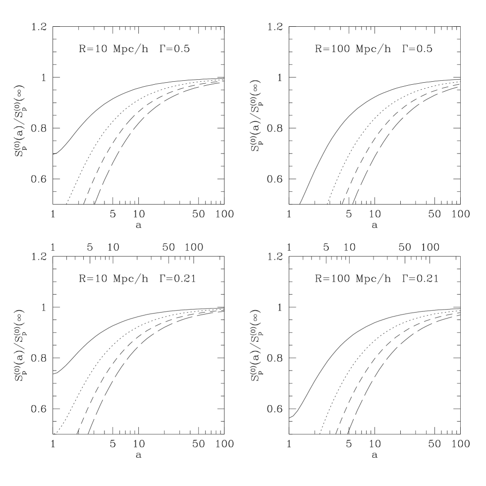
Figure 7: The ratio of the tree-level $S_{p}$ parameters at scale factor $a$ to their asymptotic exact dynamics values for CDM models as a function of scale factor $a$. Top panels correspond to a $\Gamma=0.5$ CDM model at smoothing scales $R=10,100$ h^-1Mpc, and bottom panels show the corresponding results for a $\Gamma=0.21$ CDM model. Line styles correspond to $S_{3}$ (solid), $S_{4}$ (dotted), $S_{5}$ (short-dashed), and $S_{6}$ (long-dashed). The upper axes in the bottom panels denote the scale factor $a$ for $\Omega(a)=0.3$, with $\Lambda=0$.

Figure 1 shows these results as a function of scale factor $a$ for different spectral indices, assuming that velocities are set as in the ZA. The plots show the ratio of $S_{p}(a)$ to its “true” asymptotic value predicted by PT, $S_{p}(\infty)$, for $3\leq p\leq 8$. The values at $a=1$ correspond to the ratio of ZA to exact dynamics $S_{p}$’s, which becomes smaller as either $p$ or $n$ increases. For the skewness, it takes as much as $a=6$ for $n=0$ to achieve 10% of the asymptotic exact PT value, whereas spectra with more large-scale power, where the ZA works better, require less expansion factors to yield the same accuracy. A similar constraint should hold for the bispectrum, the three-point function in Fourier space (Peebles 1980; Fry, Melott & Shandarin 1993; Scoccimarro et al. 1998). As $p$ increases, however, the transients become worse and at $p=8$ an expansion by a factor $a=40$ is required for $n=0$ to achieve $10\%$ accuracy in $S_{8}$. This suggests that the tails of the PDF could be quite affected by transients from initial conditions. Furthermore, for models where $\Omega<1$, the requirements on $a$ translate into requirements on the linear growth factor $D(\tau)$, which implies a more stringent constraint on $a$, i.e. an $\Omega<1$ simulation should be started earlier (at a higher redshift) than an $\Omega=1$ model. For example, an open model with $\Omega=0.3$ typically requires a factor of two higher initial redshift than for $\Omega=1$ (see Figs. 7 and  8 below).

Figure 2 shows the corresponding results for the velocity divergence $T_{p}$ parameters. We see that the effects of transients in this case is more severe than in the density field case, in particular as $n$ increases, since the initial $a=1$ values imposed by the initial conditions become quite different from the asymptotic exact PT values. For example, $n=0$ requires $a\approx 15$ for $10\%$ accuracy in $T_{3}$ (more than a factor of two larger than for $S_{3}$). The situation quickly deteriorates as $p$ increases. Again, the shape of the PDF of the velocity divergence should be quite sensitive to the presence of transients. Moreover, since statistics of the density field in redshift space contain contributions from velocities correlations, one expects that the redshift-space density field PDF will be more affected by transients than in real space.

Figures 3 and 4 show the equivalent results for initial velocities set from perturbed particle positions, Eq. (18). Comparing to the corresponding results in Figs. 1 and 2, these results show considerable improvement on the amount of expansion required to erase transients, by factors of two or three depending on the spectrum. We see that at most $a\approx 3$ is necessary to achieve $10\%$ accuracy in $S_{3}$, at least a factor two better than in the ZA velocities case. These results are in agreement with the numerical study of BGE for CDM models, with velocities assigned as in Eq. (18), in which they found that $a\approx 3$ was needed to recover the PT prediction for $S_{3}$ at scales where $n_{\rm eff}\approx-1$.

Figure 5 presents a comparison of the perturbative predictions for transients in $S_{p}$ parameters with the standard CDM numerical simulations measurements of BGE, kindly provided by E. Gaztañaga. The simulation evolved $100^{3}$ particles in a box 300 h^-1 Mpc a side. Initial velocities are set according to Eq. (18) as described in EDFW. The error bars in the measurements correspond to the variance over 10 realizations. We plot these N-body results by taking the ratio to the tree-level exact dynamics value predicted by PT, which has the advantage of reducing the main scale dependence. If there were no transients and no other sources of systematic uncertainties, all the curves would approach unity at large scales, where tree-level PT applies. Unfortunately, there are other sources of systematic uncertainties as we shall discuss below.

The different symbols correspond to different outputs of the simulation: open triangles denote initial conditions ($a=1$, $\sigma_{8}=0.24$), solid triangles ($a=1.66$, $\sigma_{8}=0.40$), open squares ($a=2.75$, $\sigma_{8}=0.66$), and solid squares ($a=4.2$, $\sigma_{8}=1.0$). The results for $S_{3}$ in the top left panel are those presented in Fig. 9 of BGE. For the initial conditions measurements (open triangles) there is some disagreement with the ZA predictions, especially at small scales, due to discreteness effects, which have not been corrected for. The initial particle arrangement is a grid, therefore the Poisson model commonly used to correct for discreteness is not necessarily a good approximation (see BGE for further discussion of this point). The second output time (solid triangles) is perhaps the best for testing the predictions of transients: discreteness corrections become much smaller due to evolution away from the initial conditions, and the system has not yet evolved long enough so that finite volume corrections are important. For $S_{3}$ we see excellent agreement with the predictions of Eq. (39a), with a small excess at small scales due to non-linear evolution away from the tree-level prediction. For $p>3$ the numerical results show a similar behavior with increased deviation at small scales due to non-linear evolution, as expected (see discussion below). For the last two outputs we see a further increase of non-linear effects at small scales, then a reasonable agreement (at least for $S_{3}$ and $S_{4}$) with the transients predictions, and lastly a decrease of the numerical results compared to the PT predictions at large scales due to finite volume effects, which increase with $\sigma_{8}$, $R$, and $p$ (Colombi, Bouchet & Schaeffer 1994; BGE; Colombi, Bouchet & Hernquist 1996, Munshi et al. 1997). For reasons of clarity, only measurements with reasonable error bars have been included, essentially as in BGE (see their Fig. 13).

The $N$-body results show a systematic overestimate of the PT predictions at small scales, i.e. $R\mathrel{\mathchoice{\lower 3.6pt\vbox{\halign{$\mathsurround=0pt\displaystyle\hfill#\hfil$\cr<\crcr\sim\crcr}}}{\lower 3.6pt\vbox{\halign{$\mathsurround=0pt\textstyle\hfill#\hfil$\cr<\crcr\sim\crcr}}}{\lower 3.6pt\vbox{\halign{$\mathsurround=0pt\scriptstyle\hfill#\hfil$\cr<\crcr\sim\crcr}}}{\lower 3.6pt\vbox{\halign{$\mathsurround=0pt\scriptscriptstyle\hfill#\hfil$\cr<\crcr\sim\crcr}}}}10$ h^-1Mpc for the last two outputs. Here we should stress that the PT predictions in this paper correspond to tree-level quantities, i.e. valid in the limit of vanishing variance, $\sigma^{2}(R)\rightarrow 0$. For a small variance, one can use one-loop PT to calculate the correction to the tree-level results, and neglecting transients one finds that in general (for $n<-1$ in the scale-free case)

$$S_{p}(R)=S_{p}^{(0)}+\sigma^{2}(R)\ S_{p}^{(2)}+\ldots,$$ (40)

where $S_{p}^{(0)}$ denotes the tree-level value and $S_{p}^{(2)}$ the one-loop correction coefficient (Scoccimarro & Frieman 1996). For $p=3$ and top-hat smoothing, $S_{3}^{(0)}=3.86$, $S_{3}^{(2)}=3.18$ for $n=-2$ (Scoccimarro 1997). For $p=4$ there are no available PT results to one-loop, but in the spherical collapse approximation (that has been recently extended to take into account loop-corrections by Fosalba & Gaztañaga (1997)), $S_{4}^{(0)}=27.56$, $S_{4}^{(2)}=63.56$ for $n_{\rm eff}=-2$. This approximation neglects tidal effects, but comparison with numerical simulations and exact PT results shows a good agreement for the $S_{p}$ parameters (Fosalba & Gaztañaga 1997). For example, the skewness one-loop coefficient $S_{3}^{(2)}=3.21$ for $n=-2$ is in excellent agreement with the exact PT result quoted above. These results show that at scales of a few h^-1Mpc for CDM models, where $n_{\rm eff}\approx-2$, one-loop corrections play a significant role even for $\sigma^{2}(R)<1$, and increasingly with $p$ (Fosalba & Gaztañaga 1997). This is the reason for the excess of scale dependence at $R\mathrel{\mathchoice{\lower 3.6pt\vbox{\halign{$\mathsurround=0pt\displaystyle\hfill#\hfil$\cr<\crcr\sim\crcr}}}{\lower 3.6pt\vbox{\halign{$\mathsurround=0pt\textstyle\hfill#\hfil$\cr<\crcr\sim\crcr}}}{\lower 3.6pt\vbox{\halign{$\mathsurround=0pt\scriptstyle\hfill#\hfil$\cr<\crcr\sim\crcr}}}{\lower 3.6pt\vbox{\halign{$\mathsurround=0pt\scriptscriptstyle\hfill#\hfil$\cr<\crcr\sim\crcr}}}}10$ h^-1Mpc in Fig. 5. Another interesting point of this exercise with one-loop corrections is to show how a late start in a simulation can mimic a “false agreement” with tree-level PT: transients tend to decrease the measured $S_{p}$’s, whereas one-loop corrections due to the finite variance tend to cancel this decrease. This may lead to the illusion that tree-level PT has a wider range of applicability than is really the case.

In Figure 5, the PT calculations include the full dependence on $\gamma_{p}(R)$ parameters. An approximation is sometimes used to calculate $S_{p}$ for $p>3$ in which $\gamma_{p}(R)=0$ for $p\geq 2$, on the grounds that this is true for scale-free spectra and CDM models have a slowly varying spectral index. Figure 6 addresses the validity of this approximation for standard CDM models. The top left panel shows $n_{\rm eff}=\gamma-3$ and the $\gamma_{p}(R)$ parameters for $2\leq p\leq 5$, whereas the top right panel shows the ratio of $S_{p}$ parameters ($4\leq p\leq 7$) calculated using $\gamma_{p}(R)=0$ for $p\geq 2$ to the full calculation. We see that the approximation works quite well at small scales, but as $R$ increases (and the regime where tree-level PT holds is reached) the approximation $\gamma_{p}(R)=0$ gradually breaks down. The bottom panels in Fig. 6 show the same calculation for a CDM model with shape parameter $\Gamma=0.21$ (which just corresponds to a shift in scale with respect to the $\Gamma=0.5$ model), and the corresponding calculation in the standard CDM model for the $T_{p}$ parameters. In this latter case, the approximation is worse than for the $S_{p}$ parameters. Note that we have suppressed the plotting of $T_{p}$ ratios beyond the point where they become negative for reasons of clarity.

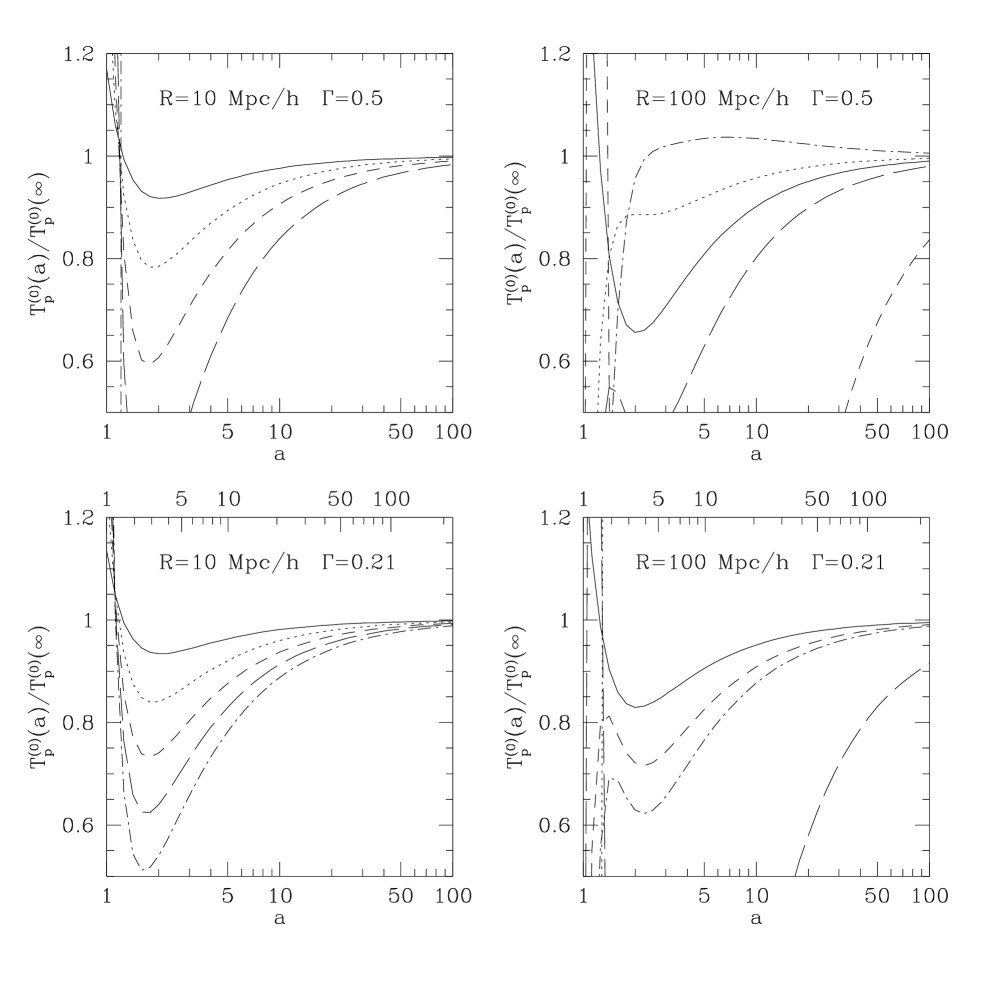
Figure 10: Same as 8, but for initial velocities set as in EDFW, see Eq. (18). The additional dot-dashed line denotes $T_{7}$.

The next two figures, Figs. 7 and 8, show the predictions of transients as a function of scale factor $a$ for $S_{p}$ and $T_{p}$ parameters respectively, at smoothing scales $R=10,100$ h^-1Mpc (left and right panels, respectively) for $\Gamma=0.5$ and $0.21$ CDM models (top and bottom panels, respectively). These calculations include the full dependence on $\gamma_{p}(R)$ parameters, and correspond to ZA initial velocities. A similar set of plots is presented in Figs. 9 and 10 for the case of velocities set as in EDFW. Comparing these two set of plots we arrive to a similar conclusion than for scale-free spectra, velocities set from perturbed particle positions lead to a faster rate of convergence to the asymptotic exact values than just pure ZA initial velocities. The latter requires a factor of about two to three more expansion away from the initial conditions to reduce transients in density and velocity statistics by the same amount. We also see that for $R=100$ h^-1Mpc, the transients are more important than for $R=10$ h^-1Mpc, as expected from the results in the scale-free case. In the bottom panels, we include upper horizontal axes which denote the scale factor $a$ for a cosmological model in which $\Omega(a)=0.3$. This serves to illustrate the fact that for models with $\Omega<1$, transients persist longer because the growth of fluctuations is governed by the linear growth factor which evolves more slowly than the scale factor. Therefore, to achieve the same accuracy regarding transient behavior, $\Omega<1$ models should be started at a higher redshift than $\Omega=1$ simulations. The results in Figs. 7-10 show that an $\Omega=0.3$ model should be started at about a factor of two larger in redshift than an $\Omega=1$ simulation. We remind the reader that this result is approximate; it depends on the assumption that $f^{2}/\Omega\approx 1$, but this approximation is better than 25% for $\Omega\geq 0.3$.

Finally, in view of these results, one is led to ask whether it is possible to decrease the magnitude of transients besides the obvious solution of starting the simulation early enough. A natural candidate to improve upon the ZA to set the initial conditions is to use second-order Lagrangian PT (hereafter 2LPT, e.g. Moutarde et al. 1991, Buchert 1992, Bouchet et al. 1995). This procedure requires minimal additional computational cost over the standard ZA scheme, as discussed in detail in Appendix D. Since 2LPT reproduces growing modes of density and velocity perturbations to second-order, there are no transients in the evolution of $S_{3}$ and $T_{3}$ parameters in this approximation. Figures 11 and 12 present the predictions for transients from 2LPT initial conditions for different spectral indices as a function of scale factor $a$ for $3\leq p\leq 8$. The details of this calculation and the analytic results are summarized in Appendix C. Compared to the corresponding results in Figs. 1 and 2 respectively (note the difference in scales), we see that 2LPT initial conditions lead to an improvement of more than an order of magnitude in the amount of expansion necessary to erase transients over the standard ZA scheme. Moreover, it yields about a factor of four improvement with respect to ZA initial conditions with velocities set from perturbed particle positions; that is, a simulation started with 2LPT initial conditions at redshift $z_{\rm start}=10$ would roughly correspond to a simulation started at $z_{\rm start}=40$ using the ZA with velocities as in EDFW, and $z_{\rm start}=100$ for a standard ZA procedure. Given that generating EDFW velocities and 2LPT initial conditions require similar additional computational costs over the ZA scheme (see Appendix D), in any case very small compared to the actual cost of running the simulation, 2LPT seems the best alternative to standard ZA methods.

5 Conclusions and Discussion

In this paper we give a perturbative analysis of the problem of transients from initial conditions when measuring moments of density and velocity fields in numerical simulations, where initial conditions are usually set using the Zel’dovich approximation (ZA). Although the ZA correctly reproduces the linear growing modes of density and velocity perturbations, non-linear growth is inaccurately represented by the ZA, because of the ZA failure to conserve momentum. This implies that it takes a non-negligible amount of time for the correct dynamics to establish the expected tree-level correlation hierarchy predicted by perturbation theory at large scales.

We focussed on one-point cumulants of the density and velocity divergence fields, characterized by the $S_{p}$ and $T_{p}$ parameters. We extended the standard formulation of perturbation theory to include to arbitrary order the transient behavior of non-linear solutions that encode the information on the amount of time needed to overcome the correlations imprinted by the initial conditions. Using these results, we calculated the full time-evolution of $S_{p}(a)$ and $T_{p}(a)$ to tree-level with top-hat smoothing as a function of scale factor $a$. These results interpolate between the initial values set by the ZA and the asymptotic values expected from the exact dynamics at large scales. More importantly, they provide a quantitative estimation of the magnitude of the effect and the amount of expansion needed to achieve a given accuracy in the determination of moments of the density and velocity fields. Needless to say, there are many other uncertainties when measuring statistics such as one-point cumulants in numerical simulations which should be properly taken into account; this has been extensively discussed in the literature (e.g. Colombi, Bouchet & Schaeffer 1994, 1995; BGE; Colombi, Bouchet & Hernquist 1996; Szapudi & Colombi 1996; Munshi et al. 1997).

We found that the magnitude of transients is determined, at a given order $p$, by the effective spectral index $n_{\rm eff}$. If initial conditions are set at $a_{0}\equiv 1$, obtaining the skewness factor $S_{3}$ ($T_{3}$) within 10$\%$ accuracy requires $a\approx 6$ ($a\approx 15$) for $n_{\rm eff}\approx 0$, whereas higher (lower) $n_{\rm eff}$ demands more (less) expansion away from initial conditions. Furthermore, these requirements become much more stringent as $p$ increases, always showing slower decay of transients for $T_{p}$ than $S_{p}$, due to velocity correlations being poorly represented by the ZA. For models with density parameter $\Omega<1$, the transients take more expansion factors to die out, since the relevant dynamical quantity that controls the growth of structure is the linear growth factor, which evolves more slowly than the scale factor. This implies, for example, that an open model where the final state corresponds to $\Omega=0.3$ requires roughly a factor of two larger expansion away from the initial conditions to erase transients than an $\Omega=1$ model. Thus, in general, numerical simulations of models with $\Omega<1$ should be started at higher redshift than critical density models to reduce transients by the same amount. We have also explored the influence of setting initial velocities on the magnitude of transients, and found that velocities set as in EDFW from the gravitational potential due to perturbed particle positions (i.e., after the ZA displacement has been applied), the time-scale of transients is reduced by a factor of two or three depending on the spectrum.

The results of the predicted transients in $S_{p}$ for $3\leq p\leq 6$ were compared with measurements in standard CDM numerical simulations by Baugh, Gaztañaga & Efstathiou (1995). We found good agreement, especially for intermediate output times where discreteness and finite volume effects are not important and tree-level PT applies over a wider range of scales. Our results show that the dependence of transients on spectral index is opposite to that of finite volume effects, which decrease with $n_{\rm eff}$ (e.g., Colombi, Bouchet & Hernquist 1996; Munshi et al. 1997). In the comparison shown in Fig. 5 we see that at late times finite volume effects start to dominate over transients, systematically decreasing $S_{5}(R)$ and $S_{6}(R)$ for $R\mathrel{\mathchoice{\lower 3.6pt\vbox{\halign{$\mathsurround=0pt\displaystyle\hfill#\hfil$\cr>\crcr\sim\crcr}}}{\lower 3.6pt\vbox{\halign{$\mathsurround=0pt\textstyle\hfill#\hfil$\cr>\crcr\sim\crcr}}}{\lower 3.6pt\vbox{\halign{$\mathsurround=0pt\scriptstyle\hfill#\hfil$\cr>\crcr\sim\crcr}}}{\lower 3.6pt\vbox{\halign{$\mathsurround=0pt\scriptscriptstyle\hfill#\hfil$\cr>\crcr\sim\crcr}}}}20$ h^-1Mpc. However, as the size of a CDM simulation box is increased and higher spectral indices are probed, transients eventually dominate over finite volume effects, since the latter become quite small as $n_{\rm eff}\rightarrow 1$.

Another interesting issue regarding transients in numerical simulations is to investigate to what extent transients are present at smaller scales. As $R$ decreases, the PT approach used here breaks down (as shown in Fig. 5 for $R\mathrel{\mathchoice{\lower 3.6pt\vbox{\halign{$\mathsurround=0pt\displaystyle\hfill#\hfil$\cr<\crcr\sim\crcr}}}{\lower 3.6pt\vbox{\halign{$\mathsurround=0pt\textstyle\hfill#\hfil$\cr<\crcr\sim\crcr}}}{\lower 3.6pt\vbox{\halign{$\mathsurround=0pt\scriptstyle\hfill#\hfil$\cr<\crcr\sim\crcr}}}{\lower 3.6pt\vbox{\halign{$\mathsurround=0pt\scriptscriptstyle\hfill#\hfil$\cr<\crcr\sim\crcr}}}}10$ h^-1Mpc in the last two outputs) since we use leading order (tree-level) PT, which yields the $S_{p}$ and $T_{p}$ parameters in the limit of vanishing variance. However, at least in the intermediate regime where the variance is of order unity and one-loop PT works well (Scoccimarro & Frieman 1996; Scoccimarro 1997), the corrections to the predictions in this paper take the form given by Eq. (40). In this case, the expected result is that transients will take longer to decay than for tree-level quantities because loop-corrections depend on higher-order non-linearities which are increasingly underestimated by the ZA. That is in fact the reason why transients in $S_{p}$ and $T_{p}$ take longer to decay as $p$ increases. On the other hand, for CDM models the spectral index decreases at smaller scales, and the magnitude of transients will decrease. As smaller scales are approached and the variance becomes larger than unity, shell-crossing becomes important and it is less clear what to expect, this depends on how much the dynamics of virializing high-density regions couples to the large-scale modes.

Since the results of transients in this work concern the statistical properties of density and velocity fields, it is likely that other statistical measures of clustering will show a similar effect, in particular those sensitive to phase correlations, where non-linear dynamics provides the leading contribution. An obvious candidate closely related to the discussion in this paper is the measurement of one-point cumulants in redshift space (Hivon et al. 1995), which can be thought as appropriate cross-correlations between density and velocity fields (Scoccimarro, Couchman & Frieman 1997). Based on the present results, one expects in this case that the $S_{p}$ parameters in redshift space will be more affected by transients that the corresponding ones in real space, since velocity correlations are more affected by transients. Other statistics sensitive to large-scale phase coherence, such as percolation studies, may show similar effects regarding transients to the ones investigated in this work.

The effect of transients also implies that one must be very careful when comparing non-linear approximations and perturbative results to numerical simulations which have not been evolved for a long enough time. In the former case, comparison among non-linear approximations usually concludes that the ZA (or modifications thereof) is a good approximation to the fully non-linear numerical simulation. These conclusions should be taken with caution if the simulation has not been started early enough so that transients from the initial conditions are still present. Also, as discussed in Section 4, when comparing numerical simulations to PT predictions, the effect of transients combined with finite values of the variance characteristic of a late simulation start tends to create the false impression that tree-level PT has a wider range of validity than is really the case.

The results in this paper should perhaps be viewed as a useful guideline for designing numerical simulations with interest in measuring higher-order statistics of density and velocity fields, as well as other measures of clustering. The main conclusion in this regard is the requirement for an early enough start to avoid undesired effects from transients, particularly for studies of clustering statistics at high redshift. Although an early start does not cause significant overhead in the time required to run a simulation because early time-steps run quite rapidly due to weak clustering, there are reasons to avoid starting a simulation at very high redshift. The faster Hubble expansion rate at earlier times demands successively shorter time-steps, but more importantly, the numerical integration of the equations of motion leads to suppressed growth of small-scale modes that becomes more significant by starting at higher redshifts (Couchman 1997). For these reasons, it is desirable to use a better approximation to generate initial conditions. A natural candidate is second-order Lagrangian PT (2LPT), which reproduces growing modes to second-order in non-linear PT. As shown in this work, this can reduce the expansion required to decay away transients by more than one order of magnitude compared to the standard ZA scheme. This is a significant improvement, particularly given that its implementation is simple and only requires minimal inexpensive modifications to widely used ZA initial conditions codes.

Appendix A Tree-Level Recursion Relations for Smoothed Vertices including Transients

We define the angular averaged smoothed kernels $\omega_{a}^{(n)}$:

$$\omega_{a}^{(n)}\equiv\int\ \Big{(}\frac{d\Omega_{1}}{4\pi}\Big{)}\ldots\Big{(}\frac{d\Omega_{n}}{4\pi}\Big{)}\ W_{1\ldots n}\ {\cal F}_{a}^{(n)}({\hbox{\BF k}}_{1},\ldots,{\hbox{\BF k}}_{n}),$$ (A1)

and similarly for the angular averaged initial conditions kernels $\eta_{a}^{(n)}$ upon replacing ${\cal F}_{a}^{(n)}$ by ${\cal I}_{a}^{(n)}$. As shown in detail by Bernardeau (1994), the operation of smoothing one-point cumulants with top-hat windows can be easily calculated due to special geometric properties. In terms of the scattering matrix elements in Eq. (26), the following properties of angular integration hold

$$\int\Big{(}\frac{d\Omega_{1}}{4\pi}\Big{)}\ \Big{(}\frac{d\Omega_{1}}{4\pi}\Big{)}\ \gamma_{121}({\hbox{\BF k}},{\hbox{\BF k}}_{1},{\hbox{\BF k}}_{2})\ W_{12} = W_{1}\ W_{2}+\frac{1}{3}\ W_{1}\ k_{2}R\ W_{2}^{\prime}$$ (A2a)

$$\int\Big{(}\frac{d\Omega_{1}}{4\pi}\Big{)}\ \Big{(}\frac{d\Omega_{1}}{4\pi}\Big{)}\ \gamma_{222}({\hbox{\BF k}},{\hbox{\BF k}}_{1},{\hbox{\BF k}}_{2})\ W_{12} = \frac{1}{3}\ W_{1}\ W_{2}+\frac{1}{6}\ W_{1}\ k_{2}R\ W_{2}^{\prime}+\frac{1}{6}\ W_{2}\ k_{1}R\ W_{1}^{\prime},$$ (A2b)

where the prime denotes a derivative (Bernardeau 1994). To prove these results, all we need is the expansion of top-hat windows such as $W_{12}$, in terms of $W_{1}$, $W_{2}$ (and their derivatives), and Legendre polynomials of the angle between ${\hbox{\BF k}}_{1}$ and ${\hbox{\BF k}}_{2}$. This, it turns out, is a straightforward application of Gegenbauer’s addition theorem for Bessel functions (e.g., Watson 1944). Then, using Eq. (A2) and the recursion relations in Eq. (23) we find:

$$\omega_{a}^{(n)}(z) = {\rm e}^{-nz}\ g_{ab}(z)\ \eta_{b}^{(n)}+\sum_{m=1}^{n-1}\int_{0}^{z}ds\ {\rm e}^{n(s-z)}\Bigg{\{}\frac{1}{3}\ g_{a1}(z-s)\ \Big{[}3\ \omega_{2}^{(m)}\ \omega_{1}^{(n-m)}+\omega_{2}^{(m)}\ \partial_{\kappa}\omega_{1}^{(n-m)}\Big{]}$$ (A3)

$$+\frac{1}{6}\ g_{a2}(z-s)\ \Big{[}2\ \omega_{2}^{(m)}\ \omega_{2}^{(n-m)}+\omega_{2}^{(m)}\ \partial_{\kappa}\omega_{2}^{(n-m)}+\partial_{\kappa}\omega_{2}^{(m)}\ \omega_{2}^{(n-m)}\Big{]}\Bigg{\}},$$

where $\kappa\equiv\ln R$ and the quantities in square brackets are evaluated at time $s$. This recursion relation (and its derivatives) can be used to obtain the smoothed vertices to arbitrary order in PT in terms of top-hat window functions and their derivatives with respect to scale, which are then straightforwardly converted to derivatives of the variance with respect to scale, yielding the $\gamma_{p}(R)$ parameters defined in Eq. (37). If we ignore transients, and assume Gaussian initial conditions, Eq. (A3) reduces to ($n>1$)

$$\omega_{a}^{(n)} = \sum_{m=1}^{n-1}\Bigg{\{}\frac{1}{3}\ \sigma_{a1}(n)\ \Big{[}3\ \omega_{2}^{(m)}\ \omega_{1}^{(n-m)}+\omega_{2}^{(m)}\ \partial_{\kappa}\omega_{1}^{(n-m)}\Big{]}$$ (A4)

$$+\frac{1}{6}\ \sigma_{a2}(n)\ \Big{[}2\ \omega_{2}^{(m)}\ \omega_{2}^{(n-m)}+\omega_{2}^{(m)}\ \partial_{\kappa}\omega_{2}^{(n-m)}+\partial_{\kappa}\omega_{2}^{(m)}\ \omega_{2}^{(n-m)}\Big{]}\Bigg{\}},$$

with

$$\sigma_{ab}(n)\equiv\frac{1}{(2n+3)(n-1)}\Bigg{[}\begin{array}[]{cc}2n+1&2\\ 3&2n\end{array}\Bigg{]}.$$ (A5)

If we further assume no smoothing, Eq. (A4) yields

$$\omega_{a}^{(n)}=\sigma_{ab}(n)\ \bar{\gamma}_{bcd}\sum_{m=1}^{n-1}\omega_{c}^{(m)}\ \omega_{d}^{(n-m)},$$ (A6)

where $\bar{\gamma}_{121}=1$, $\bar{\gamma}_{222}=1/3$, and zero otherwise, which is the limit of Eq. (A2) as the smoothing scale goes to zero, $R\rightarrow 0$. This simple recursion relation is an alternative method to reproduce the well-known results for unsmoothed vertices usually obtained using the spherical collapse approximation, i.e. $\nu_{2}=34/21$, $\nu_{3}=682/189$, $\nu_{4}=446440/43659$, …, $\mu_{2}=26/21$, $\mu_{3}=142/63$, $\mu_{4}=236872/43659$, and so on (Bernardeau 1992).

Appendix B Results for Transients in Kurtosis and Pentosis Factors

In this appendix, we present results for the transients in $S_{4},T_{4},S_{5}$ and $T_{5}$ from ZA initial conditions, for standard ZA velocities and initial velocities as in EDFW, set from perturbed particle positions (Eq. (18)). For $p=4$, evaluation of Eq. (LABEL:S4res) using the methods described in Appendix A leads to

$$S_{4}(a) = {{60712}\over{1323}}-{{62\ \gamma}\over 3}+{{7\ {\gamma^{2}}}\over 3}-{{2\ {\gamma_{2}}}\over 3}-{{816}\over{35\,a}}+{{28\ \gamma}\over{5\,a}}+{{184}\over{75\,{a^{2}}}}+{{1312}\over{245\,{a^{{7\over 2}}}}}-{{8\ \gamma}\over{5\,{a^{{7\over 2}}}}}-{{1504}\over{4725\,{a^{{9\over 2}}}}}+{{192}\over{1225\,{a^{7}}}},$$

$$T_{4}(a) = {{12088}\over{441}}-{{338\ \gamma}\over{21}}+{{7\ {\gamma^{2}}}\over 3}-{{2\ {\gamma_{2}}}\over 3}-{{624}\over{35\,a}}+{{28\ \gamma}\over{5\,a}}+{{184}\over{75\,{a^{2}}}}-{{1192}\over{245\,{a^{{7\over 2}}}}}+{{64\ \gamma}\over{35\,{a^{{7\over 2}}}}}+{{752}\over{1575\,{a^{{9\over 2}}}}}+{{432}\over{1225\,{a^{7}}}},$$

where the $\gamma_{p}$ parameters are defined in Eq. (37). For $a=1$, these expressions reduce to the initial kurtosis factors given by the ZA, and at late times they approach the asymptotic exact values (Bernardeau 1994). Similarly, for EDFW initial velocities we obtain instead

$$S_{4}(a) = S_{4}(\infty)-{{272}\over{35\,a}}+{{28\ \gamma}\over{15\,a}}+{8\over{225\,{a^{2}}}}-{{5248}\over{735\,{a^{{7\over 2}}}}}+{{32\ \gamma}\over{15\,{a^{{7\over 2}}}}}-{{5056}\over{4725\,{a^{{9\over 2}}}}}+{{1024}\over{3675\,{a^{7}}}},$$ (B3)

$$T_{4}(a) = T_{4}(\infty)-{{208}\over{35\,a}}+{{28\ \gamma}\over{15\,a}}+{8\over{225\,{a^{2}}}}+{{4768}\over{735\,{a^{{7\over 2}}}}}-{{256\ \gamma}\over{105\,{a^{{7\over 2}}}}}+{{2528}\over{1575\,{a^{{9\over 2}}}}}+{{768}\over{1225\,{a^{7}}}},$$ (B4)

where $S_{4}(\infty)$ and $T_{4}(\infty)$ denote the asymptotic exact-dynamics values given by the first four terms in Eqs. (B). For $p=5$, Eq. (35) yields for the pentosis parameters from standard ZA initial velocities

$$S_{5}(a) = {{200575880}\over{305613}}-{{1847200\ \gamma}\over{3969}}+{{6940\ {\gamma^{2}}}\over{63}}-{{235\ {\gamma^{3}}}\over{27}}-{{1490\ {\gamma_{2}}}\over{63}}+{{50\ \gamma\ {\gamma_{2}}}\over 9}-{{10\ {\gamma_{3}}}\over{27}}$$ (B5)

$$- {{74584}\over{147\,a}}+{{252\ \gamma}\over a}-{{94\ {\gamma^{2}}}\over{3\,a}}+{{20\ {\gamma_{2}}}\over{3\,a}}+{{7208}\over{63\,{a^{2}}}}-{{1352\ \gamma}\over{45\,{a^{2}}}}-{{1384}\over{225\,{a^{3}}}}+{{317104}\over{3087\,{a^{{7\over 2}}}}}-{{8984\ \gamma}\over{147\,{a^{{7\over 2}}}}}+{{188\ {\gamma^{2}}}\over{21\,{a^{{7\over 2}}}}}$$

$$- {{40\ {\gamma_{2}}}\over{21\,{a^{{7\over 2}}}}}-{{98656}\over{3969\,{a^{{9\over 2}}}}}+{{3296\ \gamma}\over{405\,{a^{{9\over 2}}}}}+{{17504}\over{17325\,{a^{{{11}\over 2}}}}}+{{1944}\over{343\,{a^{7}}}}-{{512\ \gamma}\over{245\,{a^{7}}}}+{{4352}\over{11025\,{a^{8}}}}+{{768}\over{8575\,{a^{{{21}\over 2}}}}},$$

$$T_{5}(a) = {{94262120}\over{305613}}-{{161440\ \gamma}\over{567}}+{{260\ {\gamma^{2}}}\over 3}-{{235\ {\gamma^{3}}}\over{27}}-{{130\ {\gamma_{2}}}\over 7}+{{50\ \gamma\ {\gamma_{2}}}\over 9}-{{10\ {\gamma_{3}}}\over{27}}$$ (B6)

$$- {{14792}\over{49\,a}}+{{4108\ \gamma}\over{21\,a}}-{{94\ {\gamma^{2}}}\over{3\,a}}+{{20\ {\gamma_{2}}}\over{3\,a}}+{{5512}\over{63\,{a^{2}}}}-{{1352\ \gamma}\over{45\,{a^{2}}}}-{{1384}\over{225\,{a^{3}}}}-{{68888}\over{1029\,{a^{{7\over 2}}}}}+{{1012\ \gamma}\over{21\,{a^{{7\over 2}}}}}-{{26\ {\gamma^{2}}}\over{3\,{a^{{7\over 2}}}}}$$

$$+ {{40\ {\gamma_{2}}}\over{21\,{a^{{7\over 2}}}}}+{{92072}\over{3969\,{a^{{9\over 2}}}}}-{{26248\ \gamma}\over{2835\,{a^{{9\over 2}}}}}-{{8752}\over{5775\,{a^{{{11}\over 2}}}}}+{{1944}\over{343\,{a^{7}}}}-{{96\ \gamma}\over{35\,{a^{7}}}}+{{1088}\over{1225\,{a^{8}}}}-{{2592}\over{8575\,{a^{{{21}\over 2}}}}},$$

whereas for EDFW initial velocities we get

$$S_{5}(a) = S_{5}(\infty)-{{74584}\over{441\,a}}+{{84\ \gamma}\over a}-{{94\ {\gamma^{2}}}\over{9\,a}}+{{20\ {\gamma_{2}}}\over{9\,a}}+{{136}\over{27\,{a^{2}}}}-{{184\ \gamma}\over{135\,{a^{2}}}}-{{352}\over{225\,{a^{3}}}}-{{1268416}\over{9261\,{a^{{7\over 2}}}}}+{{35936\ \gamma}\over{441\,{a^{{7\over 2}}}}}$$

$$- {{752\ {\gamma^{2}}}\over{63\,{a^{{7\over 2}}}}}+{{160\ {\gamma_{2}}}\over{63\,{a^{{7\over 2}}}}}-{{88960}\over{3969\,{a^{{9\over 2}}}}}+{{2624\ \gamma}\over{405\,{a^{{9\over 2}}}}}-{{14272}\over{7425\,{a^{{{11}\over 2}}}}}+{{3456}\over{343\,{a^{7}}}}-{{8192\ \gamma}\over{2205\,{a^{7}}}}+{{99328}\over{33075\,{a^{8}}}}-{{16384}\over{77175\,{a^{{{21}\over 2}}}}},$$

$$T_{5}(a) = T_{5}(\infty)-{{14792}\over{147\,a}}+{{4108\ \gamma}\over{63\,a}}-{{94\ {\gamma^{2}}}\over{9\,a}}+{{20\ {\gamma_{2}}}\over{9\,a}}+{{104}\over{27\,{a^{2}}}}-{{184\ \gamma}\over{135\,{a^{2}}}}-{{352}\over{225\,{a^{3}}}}+{{275552}\over{3087\,{a^{{7\over 2}}}}}-{{4048\ \gamma}\over{63\,{a^{{7\over 2}}}}}$$

$$+ {{104\ {\gamma^{2}}}\over{9\,{a^{{7\over 2}}}}}-{{160\ {\gamma_{2}}}\over{63\,{a^{{7\over 2}}}}}+{{89024}\over{3969\,{a^{{9\over 2}}}}}-{{24112\ \gamma}\over{2835\,{a^{{9\over 2}}}}}+{{7136}\over{2475\,{a^{{{11}\over 2}}}}}+{{3456}\over{343\,{a^{7}}}}-{{512\ \gamma}\over{105\,{a^{7}}}}+{{24832}\over{3675\,{a^{8}}}}+{{6144}\over{8575\,{a^{{{21}\over 2}}}}},$$

where $S_{5}(\infty)$ and $T_{5}(\infty)$ denote denote the asymptotic exact-dynamics values given by the first line in Eqs. (B5) and (B6).

Appendix C Results for Transients from Second-Order Lagrangian PT Initial Conditions

To calculate the properties of initial conditions in 2LPT, it is convenient to take advantage of the results by Munshi, Sahni & Starobinsky (1994), who derived the density and velocity divergence vertex generating functions in 2LPT for the case in which smoothing effects are neglected. The effects of smoothing can then be included by the mapping given by Bernardeau (1994b). We refer the reader to these papers for details, here we just present the results of these calculations including the effects of transients. For simplicity, we just display results assuming $\gamma_{p}=0$ for $p\geq 2$. The skewness parameters, $S_{3}$ and $T_{3}$ do not show any transient behavior in 2LPT, since these are reproduced exactly. For the kurtosis factors we have:

$$S_{4}(a)=S_{4}(\infty)-{{184}\over{105\,{a^{2}}}}+{{736}\over{945\,{a^{{9\over 2}}}}},$$ (C1)

$$T_{4}(a)=T_{4}(\infty)-{{184}\over{105\,{a^{2}}}}-{{368}\over{315\,{a^{{9\over 2}}}}},$$ (C2)

whereas for $p=5$ we obtain:

$$S_{5}(a) = S_{5}(\infty)-{{25024}\over{441\,{a^{2}}}}+{{920\ \gamma}\over{63\,{a^{2}}}}+{{320}\over{441\,{a^{3}}}}+{{85376}\over{3969\,{a^{{9\over 2}}}}}-{{3680\ \gamma}\over{567\,{a^{{9\over 2}}}}},+{{12800}\over{4851\,{a^{{{11}\over 2}}}}}$$ (C3)

$$T_{5}(a) = T_{5}(\infty)-{{19136}\over{441\,{a^{2}}}}+{{920\ \gamma}\over{63\,{a^{2}}}}+{{320}\over{441\,{a^{3}}}}-{{83536}\over{3969\,{a^{{9\over 2}}}}}+{{4600\ \gamma}\over{567\,{a^{{9\over 2}}}}}-{{6400}\over{1617\,{a^{{{11}\over 2}}}}}.$$ (C4)

Finally, the case $p=6$ yields:

$$S_{6}(a) = S_{6}(\infty)-{{16275904}\over{9261\,{a^{2}}}}+{{134872\ \gamma}\over{147\,{a^{2}}}}-{{7544\ {\gamma^{2}}}\over{63\,{a^{2}}}}+{{108800}\over{3087\,{a^{3}}}}-{{4160\ \gamma}\over{441\,{a^{3}}}}+{{50888}\over{2205\,{a^{4}}}}+{{5567104}\over{9261\,{a^{{9\over 2}}}}}$$ (C5)

$$-{{203872\ \gamma}\over{567\,{a^{{9\over 2}}}}}+{{30176\ {\gamma^{2}}}\over{567\,{a^{{9\over 2}}}}}+{{1280000}\over{11319\,{a^{{{11}\over 2}}}}}-{{166400\ \gamma}\over{4851\,{a^{{{11}\over 2}}}}}-{{3786688}\over{601965\,{a^{{{13}\over 2}}}}}+{{67712}\over{19845\,{a^{9}}}},$$

$$T_{6}(a) = T_{6}(\infty)-{{357696}\over{343\,{a^{2}}}}+{{313352\ \gamma}\over{441\,{a^{2}}}}-{{7544\ {\gamma^{2}}}\over{63\,{a^{2}}}}+{{83200}\over{3087\,{a^{3}}}}-{{4160\ \gamma}\over{441\,{a^{3}}}}+{{50888}\over{2205\,{a^{4}}}}-{{11778944}\over{27783\,{a^{{9\over 2}}}}}$$ (C6)

$$+{{418784\ \gamma}\over{1323\,{a^{{9\over 2}}}}}-{{33304\ {\gamma^{2}}}\over{567\,{a^{{9\over 2}}}}}-{{3904000}\over{33957\,{a^{{{11}\over 2}}}}}+{{217600\ \gamma}\over{4851\,{a^{{{11}\over 2}}}}}+{{1893344}\over{200655\,{a^{{{13}\over 2}}}}}+{{16928}\over{2205\,{a^{9}}}}.$$

Appendix D Lagrangian Perturbation Theory

In this appendix we present the results needed to implement 2LPT initial conditions in numerical simulations. These perturbative results are not new and have been reported before in the literature (e.g. Buchert et al. 1994, Bouchet et al. 1995), but they are collected and summarized here with emphasis on the practical issues to ease the implementation by interested readers. In particular, Buchert et al. (1994) present the necessary results to implement third-order Lagrangian PT (3LPT) solutions. However, a similar calculation to that in Appendix C shows that this only improves over 2LPT by a factor of two or so in the expansion required to erase transients. Given the additional complexity of 3LPT, which involves solving three additional Poisson equations, it does not appear worthwhile to consider.

D.1 Basic Results of Second-Order Lagrangian PT

In Lagrangian PT, the object of interest is the displacement field ${\bf\Psi}({\hbox{\BF q}})$ which maps the initial particle positions q into the final Eulerian particle positions x,

$${\hbox{\BF x}}={\hbox{\BF q}}+{\bf\Psi}({\hbox{\BF q}}).$$ (D1)

The equation of motion for particle trajectories ${\hbox{\BF x}}(\tau)$ is

$$\frac{d^{2}{\hbox{\BF x}}}{d\tau^{2}}+{\cal H}(\tau)\ \frac{d{\hbox{\BF x}}}{d\tau}=-{\bf\nabla}\Phi,$$ (D2)

where $\Phi$ denotes the gravitational potential, and ${\bf\nabla}$ the gradient operator in Eulerian coordinates x. Taking the divergence of this equation we obtain a closed equation for the displacement field

$$J({\hbox{\BF q}},\tau)\ {\bf\nabla}\cdot\Big{[}\frac{d^{2}{\hbox{\BF x}}}{d\tau^{2}}+{\cal H}(\tau)\ \frac{d{\hbox{\BF x}}}{d\tau}\Big{]}=\frac{3}{2}\Omega{\cal H}^{2}(J-1),$$ (D3)

where we have used Poisson equation together with the fact that $1+\delta({\hbox{\BF x}})=J^{-1}$, and the Jacobian $J({\hbox{\BF q}},\tau)$ is the determinant

$$J({\hbox{\BF q}},\tau)\equiv{\rm Det}\Big{(}\delta_{ij}+\Psi_{i,j}\Big{)},$$ (D4)

where $\Psi_{i,j}\equiv\partial\Psi_{i}/\partial{\hbox{\BF q}}_{j}$. Equation (D3) can be fully rewritten in terms of Lagrangian coordinates by using that ${\bf\nabla}_{i}=(\delta_{ij}+\Psi_{i,j})^{-1}{\bf\nabla}_{q_{j}}$, where ${\bf\nabla}_{q}\equiv\partial/\partial{\hbox{\BF q}}$ denotes the gradient operator in Lagrangian coordinates. The resulting non-linear equation for ${\bf\Psi}({\hbox{\BF q}})$ is then solved perturbatively, expanding about its linear solution, the Zel’dovich (1970) approximation

$${\bf\nabla}_{q}\cdot{\bf\Psi}^{(1)}=-D_{1}(\tau)\ \delta({\hbox{\BF q}}),$$ (D5)

which incorporates the kinematic aspect of the collapse of fluid elements in Lagrangian space. Here $\delta({\hbox{\BF q}})$ denotes the (Gaussian) density field imposed by the initial conditions and $D_{1}(\tau)$ is the linear growth factor, which obeys Eq. (7). The solution to second order describes the correction to the ZA displacement due to gravitational tidal effects and reads

$${\bf\nabla}_{q}\cdot{\bf\Psi}^{(2)}=\frac{1}{2}D_{2}(\tau)\sum_{i\neq j}(\Psi_{i,i}^{(1)}\Psi_{j,j}^{(1)}-\Psi_{i,j}^{(1)}\Psi_{j,i}^{(1)}),$$ (D6)

(e.g., Bouchet et al. 1995) where $D_{2}(\tau)$ denotes the second-order growth factor, which for $0.1\leq\Omega\leq 3$ ($\Lambda=0$) obeys

$$D_{2}(\tau)\approx-\frac{3}{7}D_{1}^{2}(\tau)\ \Omega^{-2/63}\approx-\frac{3}{7}D_{1}^{2}(\tau)$$ (D7)

to better than 0.5% and 7%, respectively (Bouchet et al. 1995), whereas for flat models with non-zero cosmological constant $\Lambda$ we have for $0.01\leq\Omega\leq 1$

$$D_{2}(\tau)\approx-\frac{3}{7}D_{1}^{2}(\tau)\ \Omega^{-1/143}\approx-\frac{3}{7}D_{1}^{2}(\tau),$$ (D8)

to better than 0.6% and 2.6%, respectively (Bouchet et al. 1995). Since Lagrangian solutions up to second-order are curl-free, it is convenient to define Lagrangian potentials $\phi^{(1)}$ and $\phi^{(2)}$ so that in 2LPT

$${\hbox{\BF x}}({\hbox{\BF q}})={\hbox{\BF q}}-D_{1}\ {\bf\nabla}_{q}\phi^{(1)}+D_{2}\ {\bf\nabla}_{q}\phi^{(2)},$$ (D9)

and the velocity field then reads ($t$ denotes cosmic time)

$${\bf v}\equiv\frac{d{\hbox{\BF x}}}{dt}=-D_{1}\ f_{1}\ H\ {\bf\nabla}_{q}\phi^{(1)}+D_{2}\ f_{2}\ H\ {\bf\nabla}_{q}\phi^{(2)},$$ (D10)

where $H$ is the Hubble constant, and the logarithmic derivatives of the growth factors $f_{i}\equiv(d\ln D_{i})/(d\ln a)$ can be approximated for open models with $0.1\leq\Omega\leq 1$ by

$$f_{1}\approx\Omega^{3/5},\ \ \ \ \ f_{2}\approx 2\ \Omega^{4/7},$$ (D11)

to better than 2% (Peebles 1976) and 5% (Bouchet et al. 1995), respectively. For flat models with non-zero cosmological constant $\Lambda$ we have for $0.01\leq\Omega\leq 1$

$$f_{1}\approx\Omega^{5/9},\ \ \ \ \ f_{2}\approx 2\ \Omega^{6/11},$$ (D12)

to better than 10% and 12%, respectively (Bouchet et al. 1995). The accuracy of these two fits improves significantly for $\Omega\geq 0.1$, in the range relevant for the present purposes. The time-independent potentials in Eqs. (D9) and (D10) obey the following Poisson equations (Buchert et al. 1994)

$${\bf\nabla}_{q}^{2}\phi^{(1)}({\hbox{\BF q}}) = \delta({\hbox{\BF q}}),$$ (D13a)

$${\bf\nabla}_{q}^{2}\phi^{(2)}({\hbox{\BF q}}) = \sum_{i>j}[\phi_{,ii}^{(1)}({\hbox{\BF q}})\ \phi_{,jj}^{(1)}({\hbox{\BF q}})-(\phi_{,ij}^{(1)}({\hbox{\BF q}}))^{2}],$$ (D13b)

D.2 Setting up Second-Order Lagrangian PT Initial Conditions

We now have all the elements to describe a simple prescription to implement 2LPT initial conditions (hereafter, a tilde denotes a Fourier-space quantity):

- A Gaussian density field, $\tilde{\delta}({\hbox{\BF k}})$ is generated in Fourier space from the desired linear power spectrum, and therefore $\tilde{\phi}^{(1)}({\hbox{\BF k}})$ follows from Eq. (D13a) in Fourier space.

- Inverse fast Fourier transform (FFT) of $\tilde{\phi}^{(1)}({\hbox{\BF k}})$ yields $\phi^{(1)}({\hbox{\BF q}})$ on the grid of unperturbed particle positions.

- ${\bf\nabla}_{q}\phi^{(1)}$ is obtained by differencing $\phi^{(1)}({\hbox{\BF q}})$ along the three directions, giving the necessary ingredients to displace particles and assign velocities according to the ZA. So far, this is the usual procedure.

- The array ${\bf\nabla}_{q}\phi^{(1)}$ can be stored temporarily in the array reserved for the velocities assignment. Then we need three additional arrays of dimension $N_{\rm grid}$ (where $N_{\rm grid}$ is the dimension of the grid used to set up the initial conditions, usually equal to the number of particles) to calculate the source term in Eq. (D13b). By differencing the components of the array ${\bf\nabla}_{q}\phi^{(1)}$ in a diagonal fashion we obtain the diagonal terms ${\bf\nabla}^{2}_{11}\phi^{(1)}$, ${\bf\nabla}^{2}_{22}\phi^{(1)}$, and ${\bf\nabla}^{2}_{33}\phi^{(1)}$, each stored in a $N_{\rm grid}$ array, which are then multiplied together to give the first contribution to the source term in Eq. (D13b). The second contribution, consisting of the non-diagonal terms $\phi_{,ij}^{(1)}({\hbox{\BF q}})$ in Eq. (D13b), is obtained by simply differencing and accumulating in turn, without the need of additional memory space. This yields the source term to the second Poisson equation on the grid of unperturbed particle positions, stored in an array of dimension $N_{\rm grid}$.

- FFT of this source term, solving Eq. (D13b) for $\tilde{\phi}^{(2)}({\hbox{\BF k}})$ in Fourier space, and inverse FFT yields the second-order potential $\phi^{(2)}({\hbox{\BF q}})$ on the grid of unperturbed particle positions.

- The $\phi^{(2)}({\hbox{\BF q}})$ array is then differenced along one direction (recycling one of the two usable $N_{\rm grid}$ arrays to thus store ${\bf\nabla}_{1}\phi^{(2)}$) and then particles are displaced and velocities assigned along the direction in question by combining ${\bf\nabla}_{1}\phi^{(1)}$ and ${\bf\nabla}_{1}\phi^{(2)}$ according to Eqs. (D9) and (D10). The same procedure is applied in turn to the two remaining directions.

We therefore see that the additional requirements for 2LPT initial conditions generation over the standard ZA scheme is basically two FFT’s, a $3\times N_{\rm grid}$ array, and differencing of the Lagrangian potentials. These are indeed very modest by speed and memory considerations, especially given the fact that setting up initial conditions is always a small fraction of the cost of running the numerical simulation. In view of the substantial improvement (more than one order of magnitude) on the required amount of expansion to erase transients from initial conditions, it seems well worth the minimal extra effort.

Figure 1: The ratio of the tree-level $S_{p}$ parameters at scale factor $a$ to their asymptotic exact dynamics value for scale-free initial spectra with different spectral indices: $S_{3}$ (solid lines), $S_{4}$ (dotted), $S_{5}$ (short-dashed), $S_{6}$ (long-dashed), $S_{7}$ (dot-short-dashed), and $S_{8}$ (dot-long-dashed). The values at $a=1$ represent those set by the ZA initial conditions. For cosmological models with $\Omega<1$, the horizontal axis becomes the linear growth factor.

Figure 2: Same as Figure 1, but for the $T_{p}$ parameters.

Figure 3: Same as Figure 1, but for initial velocities set as in EDFW, see Eq. (18).

Figure 4: Same as Figure 2, but for initial velocities set as in EDFW, see Eq. (18).

Figure 5: Symbols show the ratio of the $S_{p}$ parameters at scale factor $a$ measured in SCDM numerical simulations (Baugh, Gaztañaga & Efstathiou 1995) to their asymptotic tree-level exact dynamics value as a function of smoothing scale $R$. Symbols represent $a=1$ (open triangles), $a=1.66$ (filled triangles), $a=2.75$ (open squares) and $a=4.2$ (filled squares). Error bars denote the variance of measurements in 10 realizations. Solid lines correspond to the predictions of transients in tree-level PT, expected to be valid at large scales.

Figure 6: The top left panel shows the $\gamma_{p}$ parameters as a function of smoothing scale $R$ for a $\Gamma=0.5$ CDM model. The solid line corresponds to $n_{\rm eff}(R)\equiv\gamma(R)-3$, and $\gamma_{2}$ (dotted line), $\gamma_{3}$ (short-dashed), $\gamma_{4}$ (long-dashed), $\gamma_{5}$ (dot-dashed). The top right panel shows the ratio of the $S_{p}$ parameters to those calculated by setting $\gamma_{p}=0$ for $p\geq 2$ as a function of scale. Line-styles denote $S_{4}$ (solid), $S_{5}$ (dotted), $S_{6}$ (short-dashed) and $S_{7}$ (long-dashed). The left bottom panel shows the analogous calculation for a $\Gamma=0.21$ CDM model. Right bottom panel presents a similar result for the $T_{p}$ parameters in the $\Gamma=0.5$ CDM model.

Figure 8: Same as Fig. 7, but for the $T_{p}$ parameters.

Figure 9: Same as Fig. 7, but for initial velocities set as in EDFW, see Eq. (18). The additional dot-dashed line denotes $S_{7}$.

Figure 11: Same as Fig. 1, but for initial conditions set using second-order Lagrangian perturbation theory. Compare with Figs. 1 and 3 (note the difference in plot scales).

Figure 12: Same as Fig. 2, but for the $T_{p}$ parameters. Compare with Figs. 2 and 4

References

- (1)
- (2) Balian, R., & Schaeffer, R. 1989, A & A, 220, 1
- (3)
- (4) Baugh, C. M., Gaztañaga, E., & Efstathiou, G. 1995, MNRAS 274, 1049 (BGE)
- (5)
- (6) Bernardeau, F. 1992, ApJ, 392, 1
- (7)
- (8) Bernardeau, F. 1994, ApJ, 433, 1
- (9)
- (10) Bernardeau, F. 1994b, A & A, 291, 697
- (11)
- (12) Bernardeau, F., & Kofman, L. 1995, ApJ, 443, 479
- (13)
- (14) Bernardeau, F., van de Weygaert, R., Hivon, E., & Bouchet F. R. 1997, MNRAS, 290, 566
- (15)
- (16) Boschán, P., Szapudi, I., & Szalay, A.S. 1994, ApJS, 93, 65
- (17)
- (18) Buchert, T. 1992, MNRAS, 254, 729
- (19)
- (20) Buchert, T., Melott, A. L., & Weiss, A. G. 1994, A & A, 288, 349
- (21)
- (22) Bouchet, F. R., Juszkiewicz, R., Colombi, S., Pellat, R., & 1992, ApJ, 394, L5
- (23)
- (24) Bouchet, F. R., Colombi, S., Hivon, E., & Juszkiewicz, R. 1995, A&A, 296, 575
- (25)
- (26) Catelan, P., Lucchin, F. , Matarrese, S., & Moscardini, L. 1995, MNRAS, 276, 39
- (27)
- (28) Catelan, P., & Moscardini, L. 1994, ApJ, 426, 14
- (29)
- (30) Chodorowski, M. J., & Bouchet, F. R. 1996, MNRAS, 279, 557
- (31)
- (32) Colombi, S., Bouchet, F. R., & Schaeffer, R. 1994, A&A, 281, 301
- (33)
- (34) Colombi, S., Bouchet, F. R., & Schaeffer, R. 1995, ApJS, 96, 401
- (35)
- (36) Colombi, S., Bouchet, F. R., & Hernquist, L. 1996, ApJ, 465, 14
- (37)
- (38) Couchman, H. M. P. & Peebles, P. J. E. 1997, preprint, astro-ph/9708230.
- (39)
- (40) Couchman, H. M. P. 1997, private communication
- (41)
- (42) Efstathiou, G., Davis, M., Frenk, C. S., & White, S. D. M. 1985, ApJS, 57, 241 (EDFW)
- (43)
- (44) Fosalba, P., & Gaztañaga, E. 1997, in preparation
- (45)
- (46) Fry, J. N. 1984, ApJ, 279, 499
- (47)
- (48) Fry, J. N., Melott, A. M. & Shandarin, S. F. 1993, ApJ, 412, 504
- (49)
- (50) Fry, J. N., & Scherrer, R. J. 1994, ApJ, 429, 36
- (51)
- (52) Gaztañaga, E. 1994, ApJ, 268, 913
- (53)
- (54) Gaztañaga, E. & Baugh, C. M. 1995, MNRAS, 273, L1
- (55)
- (56) Goroff, M. H., Grinstein, B., Rey, S.-J., & Wise, M. 1986, ApJ, 311, 6
- (57)
- (58) Grinstein, B. & Wise, M. 1987, ApJ, 320, 448
- (59)
- (60) Hivon, E., Bouchet, F. R., Colombi, S., & Juszkiewicz, R. 1995, A&A, 298, 643
- (61)
- (62) Hui, L., & Bertschinger, E. 1996, ApJ, 471, 1
- (63)
- (64) Jain, B. & Bertschinger, E. 1994, ApJ, 431, 495
- (65)
- (66) Juszkiewicz, R., Bouchet, F. R., & Colombi, S. 1993, ApJ, 412, L9
- (67)
- (68) Juszkiewicz, R., Weinberg, D. H., Amsterdamski, P., Chodorowski, M., & Bouchet, F. R. 1995, ApJ, 442, 39
- (69)
- (70) Klypin, A. A. & Shandarin, S. F. 1983, MNRAS, 204, 891
- (71)
- (72) Łokas, E. L., Juszkiewicz, R., Weinberg, D. H. & Bouchet, F. R. 1995, MNRAS, 274, 730
- (73)
- (74) Martel, H., & Freudling, W. 1991, ApJ, 371, 1
- (75)
- (76) Moutarde, F., Alimi, J. M., Bouchet, F. R., Pellat, R., & Ramani, A., 1991, ApJ, 382, 377
- (77)
- (78) Munshi, D., & Starobinsky, A. A. 1994, ApJ, 428, 433
- (79)
- (80) Munshi, D., Sahni, V., & Starobinsky, A. A. 1994, ApJ, 436, 517
- (81)
- (82) Munshi, D., Bernardeau, F., Melott, A. L., & Schaeffer, R. 1997, submitted to MNRAS, astro-ph/9707009 .
- (83)
- (84) Nusser, A., & Colberg, J. M. 1997, submitted to MNRAS, astro-ph/9705121.
- (85)
- (86) Peebles, P. J. E. 1976, ApJ, 205, 318
- (87)
- (88) Peebles, P. J. E. 1980, The Large-Scale Structure of the Universe (Princeton: Princeton Univ. Press)
- (89)
- (90) Scoccimarro, R., 1997, ApJ, 487, 1
- (91)
- (92) Scoccimarro, R. 1997b, in preparation
- (93)
- (94) Scoccimarro, R., & Frieman, J. A. 1996, ApJS, 105, 37
- (95)
- (96) Scoccimarro R., Colombi, S., Fry, J. N., Frieman, J., Hivon, E., & Melott, A., 1998, ApJ, 496, in press, astro-ph/9704075.
- (97)
- (98) Scoccimarro R., Couchman, H. M. P., & Frieman, J. 1997, in preparation.
- (99)
- (100) Szapudi, I., & Colombi, S. 1996, ApJ, 470, 131
- (101)
- (102) Szapudi, I., Meiksin, A., & Nichol, R. C. 1996, ApJ, 473, 15
- (103)
- (104) Watson, G. N. 1944, A Treatise on the Theory of Bessel Functions, 2nd ed., Cambridge University Press
- (105)
- (106) Wise, M. B. 1988, in The Early Universe, ed. W. G. Unruh & G. W. Semenoff (Dordrecht: Reidel), 215
- (107)
- (108) Zel’dovich, Ya. B., 1970, A&A, 5, 84
- (109)