The circumstellar shell of the post-AGB star HD 56126: the ¹²CN/¹³CN isotope ratio and fractionation

Abstract

We have detected circumstellar absorption lines of the ¹²CN and ¹³CN Violet and Red System in the spectrum of the post-AGB star HD 56126. From a synthetic spectrum analysis, we derive a Doppler broadening parameter of $b=0.51\pm 0.04$ km s^-1, ¹²CN/¹³CN$=38\pm 2$, and a lower limit of $2000$ on ¹²CN/¹⁴CN and ¹²C¹⁴N/¹²C¹⁵N. A simple chemical model has been computed of the circumstellar shell surrounding HD 56126 that takes into account the gas-phase ion-molecule reaction between CN and C⁺. From this we infer that this reaction leads to isotopic fractionation of CN. Taking into account the isotopic exchange reaction and the observed ¹²CN/¹³CN we find ¹²C/¹³C$\sim 67$ (for $T_{\rm kin}=25$ K). Our analysis suggests that ¹²CN has a somewhat higher rotational temperature than ¹³CN: $T_{\rm rot}=11.5\pm 0.6$ and $8.0\pm 0.6$ K respectively. We identify possible causes for this difference in excitation temperature, among which the $N^{\prime\prime}$ dependence of the isotopic exchange reaction.

1 Introduction

The evolution of a low-mass red giant terminates on the tip of the Asymptotic Giant Branch (AGB). The remnant, which is a carbon-oxygen core with a dilute extended convective envelope, evolves along a constant luminosity track toward the White Dwarf (WD) phase. This transition from the AGB to the WD is referred to as the post-AGB phase, or the Pre-Planetary Nebulae (PPN) phase. Since low-mass stars are the main contributors of carbon, nitrogen, and s-process elements to the interstellar medium (ISM) (Forestini & Charbonnel 1997), accurate information of the chemical composition of AGB and post-AGB stars is important. Post-AGB stars may provide useful information on the composition of the gas returned to the ISM. In particular, the fact that their spectra are much simpler than those of the cool AGB stars affords novel opportunities to infer details of the composition of AGB stellar envelopes.

The present photosphere of HD 56126 ($T_{\rm eff}=7000$ K) is carbon-rich (C/O$\simeq$1.4), metal-poor ([Fe/H]$\simeq$-1.0), and enhanced in s-process elements ([s/Fe]=1.7) (Klochkova 1995). Such an abundance pattern resembles that of carbon stars (Lambert et al. 1986, Utsumi 1970) that result from the dredge-up of nucleosynthesis products as a star evolves up the AGB. HD 56126 is the prototype of a group of post-AGB and AGB stars that exhibit absorption lines from circumstellar C₂ and CN (from now on C means ¹²C and N means ¹⁵N) in their spectra (Bakker et al. 1996 (Paper I), Bakker et al. 1997 (Paper II)). In order to facilitate further discussion, we introduce the term “C2CN” stars to refer to this group of stars. Molecules are present in the detached shell surrounding the star and the chemical composition of the dusty shell reflects the photospheric composition of the star when it was at the tip of the Asymptotic Giant Branch (TP-AGB). The molecular composition of the shell has evolved, for example a simple molecule like CN is believed to be formed as a result of photodissociation of complex molecules (in this case HCN) by the interstellar radiation field.

Excitation of the CN molecule’s X${}^{2}\Sigma^{+}$ ground state is likely controlled by absorption and re-emission of photons in the Violet (${\rm B}^{2}\Sigma^{+}\rightarrow{\rm X}^{2}\Sigma^{+}$) and Red (${\rm A}^{2}\Pi\rightarrow{\rm X}^{2}\Sigma^{+}$) System, and pure rotational transitions (principally de-excitation) in the X${}^{2}\Sigma^{+}$ state. At the low densities of the circumstellar shell, the pure rotational transitions will cool the rotational ladder below the gas kinetic temperature (sub-thermal). For a symmetric molecule without a dipole moment (e.g. C₂), pure rotational transitions are forbidden and the molecule can not efficiently cool. The excitation temperature is higher than the kinetic temperature of the gas (supra-thermal). Through measurement of the level population and modeling of the (de-)excitation processes, the CN molecule serves as a probe of the physical conditions in the shell. A molecule like CN additionally affords an opportunity to compare column densities of isotopomers, e.g. the ratio of CN to ¹³CN. In turn, understanding of the chemistry enables the isotopic ratio ¹²C/¹³C to be derived from the measured ¹²CN/¹³CN ratio.

In this paper (Paper III) we present and discuss the first measurement of the CN/¹³CN ratio and an estimate of the ¹²C/¹³C ratio and lower limits on ¹²C/¹⁴C and ¹⁴N/¹⁵N in the circumstellar shell of a post-AGB star. In Sec. 2 we discuss the observations and the dataset of equivalent widths used in our analysis. Sec. 3 goes into the details of the molecular parameters used, and Sec. 4 describes the analysis and results. A discussion of the results is presented in Sec. 5.

2 Observations and equivalent widths

High-resolution spectra were obtained with 2.7 m Harlan J. Smith telescope of the W. J. McDonald observatory and the coudé cross-dispersed echelle spectrograph (Tull et al. 1995). Spectra at a resolution $R=\lambda/\Delta\lambda\simeq 140,000$ were acquired of the ($v^{\prime}-v^{\prime\prime})=(0-0)$ band of the CN Violet System and $R\simeq 200,000$ of the (3-0) and (4-0) bands of the CN Red System. Observations were made from December 1996 to March 1997 (Table 1). The spectral resolution of the spectra was determined from the $FWHM$ of the emission lines in the accompanying ThAr arc spectrum and corrected for the intrinsic width of the ThAr emission lines.

Table 1: Log of observations.

Date $HJD$ Int. [s] $R=\frac{\lambda}{\Delta\lambda}$ $\lambda_{\rm c}$ [Å] $SNR$ Remark 29 Dec. 96 2450446.7158 6$\times$1800 200,000 7558 100 Red (3,0) + H$\alpha$ 02 Jan. 97 2450450.8708 3$\times$1800 140,000 4062 20 Violet (0,0) + Ca II H + H$\epsilon$ 28 Feb. 97 2450507.5840 6$\times$1800 140,000 4056 15 Violet (0,0) + H$\delta$ 01 Mar. 97 2450508.5696 6$\times$1800 140,000 3874 22 Violet (0,0) + H$\delta$ 03 Mar. 97 2450510.6087 8$\times$1800 200,000 6086 70 Red (3,0) + Red (4,0) Co-added spectra Violet System (0,0) 7.5 hrs 140,000 3877 35 Red System (3,0) 7.0 hrs 200,000 6945 200 Red System (4,0) 4.0 hrs 200,000 6195 90

Observations of 30 minutes have been co-added to give the final spectra for each night. All spectra were reduced using IRAF in the standard manner. Individual integrations were corrected for the velocity shift due to the Earth rotation and instrumental drift before combining them to an average spectrum. The final S/N ratio of the spectra is 35 for the Violet (0-0) band and 200 and 90 for the Red (3-0) and (4-0) bands respectively.

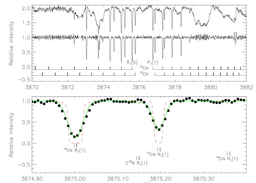
Figure 1: CN Violet System (0,0) band towards HD 56126. The upper panel shows the observed spectrum and a rectified spectrum corrected for the underlying photospheric features. The rectified spectrum contains only circumstellar lines. The lower panel shows on an expanded wavelength scale the strongest line (the R₁, R₂, and ${}^{\rm R}Q_{21}$ blend for $N^{\prime\prime}=1$), and demonstrates that we have not detected ¹⁴CN and C¹⁵N. The dashed spectrum is a synthetic spectrum computed for $b=0.51$ km s^-1 , $T_{\rm rot}=11.5$ K for CN, $T_{\rm rot}=8.0$ for the CN isotopes, and the isotope or lower limit isotope ratios as determined in this work. The solid spectrum is the synthetic spectrum convolved to our spectral resolution of $R=140,000$.

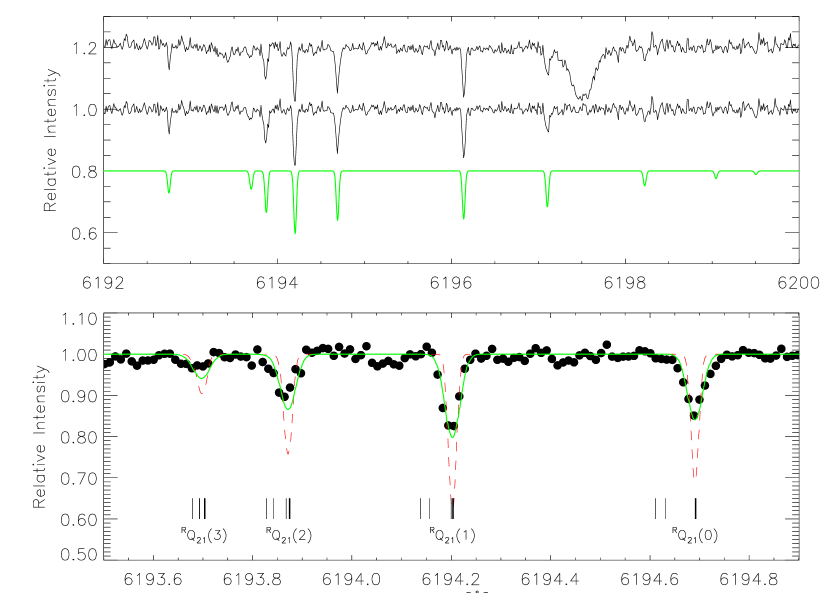
Figure 2: CN Red System (4,0) band towards HD 56126. The upper panel shows the observed spectrum (offset by 0.2), a rectified spectrum corrected for the underlying photospheric features, and convolved synthetic spectrum (offset by -0.2) The rectified spectrum contains only circumstellar lines. The lower panel shows on an expanded wavelength scale centered around the strongest line (the $\rm{}^{R}Q_{21}$(1) or R₂(1) blend) (lower panel). The dashed and solid synthetic spectrum are explained in the caption of Fig. 1. The ¹³CN (4,0) band is red-shifted by about 54 Å  and not covered by this spectrum. The solid spectrum is the synthetic spectrum convolved to our spectral resolution of $R=200,000$.

Portion of the final spectra are shown in Figs. 1 and 2. From each final spectrum we removed the molecular features and fitted a high order spline that followed all photospheric features. The observed spectrum what divided by this fit to obtain the rectified spectrum which only contains the molecular features. Circumstellar CN lines are readily distinguishable from the much broader photospheric lines of various atomic species. The equivalent widths (Tables 2 and 3) of the molecular lines were measured relative to the local continuum (taking into account stellar absorption lines). A search for ¹⁴CN and C¹⁵N of the Violet System (0,0) band was unsuccessful: an upper limit to their equivalent width is 1.5 mÅ.

HD 56126 is a pulsating star. The photospheric spectrum from the star might therefore change from one run to the other and combining the spectrum from different runs could lead to errors. We therefore have measured the equivalent width of the lines for each night separately and averaged to obtain the final equivalent width. The spectra in Figs. 1 and 2 are combined using all available data and there is no indication that the photospheric spectrum has indeed changed from one run to the next.

This high quality dataset was extended with previous data of the Red System (1,0), (2,0), and (3,0) bands (presented in Paper I), provided by spectra collected with the WHT/UES at a spectral resolution of $R\approx 50,000$. Our new measurements for the Red (3-0) band are in good agreement with measurements of Paper I. The weaker lines were only detected at our higher resolution. Our new measurements for the Red (3-0) band are in good agreement with measurements of Paper I.

Table 2: CN Violet System (0,0) with $f_{(0,0)}=0.0330$. Derived column densities are given in Table 4.

$B(N^{\prime\prime})$ $\lambda_{\rm rest}$ [Å] $\Delta\lambda$ [Å]^a $f_{N^{\prime}J^{\prime},N^{\prime\prime}J^{\prime\prime}}$ $f_{\rm eff}N$[cm^-2] $W_{\lambda}$ [mÅ] Remark CN ¹³CN ¹⁴CN C¹⁵N CN ¹³CN $\rm R_{1}$(6) 3870.666l 0.348l 0.604c 0.239c 0.0176 $0.0178N(6)$ $<2.0$ $<2.0$ $\rm R_{2}$(6) 3870.657l 0.0178 $\rm{}^{R}Q_{21}$(6) 3870.665c 0.0002 $\rm R_{1}$(5) 3871.358l 0.300l 0.550c 0.218c 0.0178 $0.0180N(5)$ $9.6\pm 0.3$ $<2.0$ $\rm R_{2}$(5) 3871.366l 0.0180 $\rm{}^{R}Q_{21}$(5) 3871.371c 0.0002 $\rm R_{1}$(4) 3872.045l 0.277l 0.497c 0.197c 0.0180 $0.0183N(4)$ $29.0\pm 0.5$ $<1.7$ too strong $\rm R_{2}$(4) 3872.053l 0.0183 $\rm{}^{R}Q_{21}$(4) 3872.058c 0.0003 $\rm R_{1}$(3) 3872.716l 0.252l 0.446c 0.176c 0.0183 $0.0189N(3)$ $25.1\pm 0.3$ $6.3\pm 0.5$ perturbed $\rm R_{2}$(3) 3872.712l 0.0189 $\rm{}^{R}Q_{21}$(3) 3872.725c 0.0006 3872.774l $10.0\pm 0.3$ perturbation $\rm R_{1}$(2) 3873.363l 0.222l 0.396c 0.156c 0.0189 $0.0198N(2)$ $37.1\pm 0.3$ $18.6\pm 0.3$ $\rm R_{2}$(2) 3873.370l 0.0198 $\rm{}^{R}Q_{21}$(2) 3873.371l 0.0009 $\rm R_{1}$(1) 3873.991l 0.192l 0.348c 0.137c 0.0198 $0.0220N(1)$ $36.7\pm 0.3$ $25.0\pm 0.3$ $\rm R_{2}$(1) 3873.996l 0.0220 $\rm{}^{R}Q_{21}$(1) 3873.998l 0.0022 $\rm R_{1}$(0) 3874.602l 0.176l 0.301c 0.119c 0.0220 $0.0330N(0)$ $36.3\pm 0.3$ $21.1\pm 0.4$ $\rm{}^{R}Q_{21}$(0) 3874.605l 0.0110 $\rm{}^{P}Q_{12}$(1) 3875.758l 0.0110 $\rm P_{1}$(1) 3875.759l 0.130o 0.212c 0.083c 0.0110 $0.0110N(1)$ $32.6\pm 0.3$ $18.4\pm 0.3$ $\rm{}^{P}Q_{12}$(2) 3876.304l 0.0022 $\rm P_{1}$(2) 3876.306l 0.105l 0.170c 0.067c 0.0132 $0.0132N(2)$ $29.0\pm 0.3$ $13.7\pm 0.3$ $\rm P_{2}$(2) 3876.308l 0.0110 $\rm{}^{P}Q_{12}$(3) 3876.830c 0.0009 $\rm P_{1}$(3) 3876.834l 0.063l 0.130c 0.050c 0.0141 $0.0141N(3)$ $27.6\pm 0.3$ $4.2\pm 0.5$ $\rm P_{2}$(3) 3876.836l 0.0132 $\rm{}^{P}Q_{12}$(4) 3877.336c 0.0006 $\rm P_{1}$(4) 3877.341l 0.056l 0.091c 0.035c 0.0147 $0.0147N(4)$ $24.1\pm 0.3$ $<1.0$ $\rm P_{2}$(4) 3877.345l 0.0141 $\rm{}^{P}Q_{12}$(5) 3877.821c 0.0003 $\rm P_{1}$(5) 3877.828l 0.028c 0.054c 0.020c 0.0150 $0.0150N(5)$ $3.9\pm 0.5$ polluted perturbed $\rm P_{2}$(5) 3877.825l 0.0147 3877.885l $<1.0$ perturbation $\rm{}^{P}Q_{12}$(6) 3878.286c 0.0002 $\rm P_{1}$(6) 3878.294l 0.008c 0.018c 0.006c 0.0152 $0.0152N(6)$ $<1.0$ $<1.0$ $\rm P_{2}$(6) 3878.300l 0.0150 a: isotopic shift relative to CN. Example: R₂(1) ¹⁴CN at 3873.996+0.348=3874.344 Å c: computed; l: laboratory data; o: spectrum bl: blended with the ¹²CN P(5) blend For lines with laboratory data: $v$(CN)$=77.5\pm 0.5$ km s^-1 and $v$(¹³CN)$=76.7\pm 1.8$ km s^-1

Table 3: CN Red System (4,0) with $f_{(4,0)}=1.09\times 10^{-4}$. Derived column densities are given in Table 4.

$B(N^{\prime\prime})$ $\lambda_{\rm rest}$ [Å] $f_{N^{\prime}J^{\prime},N^{\prime\prime}J^{\prime\prime}}\times 10^{4}$ $f_{\rm eff}\times 10^{4}N(N^{\prime\prime})$[cm^-2] $W_{\lambda}$ [mÅ] Remark $\rm{}^{S}R_{21}$(3) 6186.293l 0.101 0.058N(3) $\leq 1.5$ $\rm{}^{S}R_{21}$(2) 6187.764l 0.112 0.067N(2) $1.8\pm 0.5$ $\rm{}^{S}R_{21}$(1) 6189.397l 0.127 0.085N(1) $3.1\pm 0.5$ $\rm{}^{S}R_{21}$(0) 6191.159c 0.151 0.151N(0) $2.4\pm 0.1$ $\rm R_{2}$(3) 6192.087l 0.202 $\rm{}^{R}Q_{21}$(3) 6192.101c 0.217 0.211N(3) $\leq 1.5$ $\rm R_{2}$(2) 6192.255l 0.203 $\rm{}^{R}Q_{21}$(2) 6192.274c 0.237 0.223N(2) $5.3\pm 0.6$ $\rm R_{2}$(1) 6192.572c 0.215 $\rm{}^{R}Q_{21}$(1) 6192.605l 0.264 0.248N(1) $8.0\pm 0.2$ $\rm{}^{R}Q_{21}$(0) 6193.008l 0.363 0.363N(0) $7.2\pm 0.1$ $\rm Q_{2}$(1) 6194.485l 0.363 0.182N(1) $6.7\pm 0.1$ $\rm{}^{Q}P_{21}$(1) 6194.550c 0.091 $\rm Q_{2}$(2) 6195.467l 0.316 0.188N(2) $4.5\pm 0.5$ $\rm{}^{Q}P_{21}$(2) 6195.515c 0.102 $\rm Q_{2}$(3) 6196.622l 0.323 0.197N(3) $1.7\pm 0.2$ $\rm{}^{Q}P_{21}$(3) 6196.638c 0.103 $\rm P_{2}$(2) 6197.458l 0.091 0.036N(2) $\leq 1.5$

3 Molecular data

3.1 CN Violet System

Wavelengths for CN Violet System (0,0) were computed from the wavenumbers of Prasad et al. (1992) and the isotopic wavelengths for ¹³CN Violet System (0,0) from Jenkins & Wooldridge (1938). The isotopic shift of the ¹³CN P₁($N^{\prime\prime}=1$) blend was obtained from our observed spectrum. Lines positions not listed in these papers were computed using the molecular constants given by Prasad et al. and the standard relations for the mass dependence of the various molecular constants (cf Bernath 1995). The computed wavenumbers were in good agreement with the laboratory measurements. Predictions were extended to the isotopes ¹⁴CN and C¹⁵N. Table 2 lists the wavelength shift of the various isotopes relative to CN. The isotopic shift is the same for the three lines within one blend. For example: the ¹³CN ^RQ₂₁ (2) line is at 3873.593 Å. In all cases the index of refraction of standard air was computed using the formula given by Morton (1991).

The $f_{\rm V}$-value of the Violet System is well determined experimentally and theoretically. Theoretical calculations by Knowles et al. (1988) and Bauschlicher, Langhoff & Taylor (1988) predict $f_{\rm V}$(0-0)=0.0345 and 0.0335 respectively. An earlier calculation by Larsson, Siegbahn & $\rm\AA$gren (1983) gave $f_{\rm V}$(0-0)=0.0324. The most accurate experimental results are the measurements of the radiative lifetime of the B${}^{2}\Sigma^{+}$ state. Low rotational states of the $v^{\prime}=0$ level of the B state have measured lifetimes (in ns) of $60.8\pm 2.0$ (Luk & Bersohn 1973), $65.1\pm 0.8$ (Jackson 1974), and $66.7\pm 1.4$ (Duric, Erman & Larsson 1978). Theoretical values (including the small contribution from the B${}^{2}\Sigma^{+}\rightarrow$A${}^{2}\Pi$) are 60.7 (Knowles et al.), 62.4 (Bauschlicher et al.) and 66.6 (Larsson et al.) We adopt $f_{\rm V}(0-0)=0.033$ which is approximately the average of these various theoretical and experimental estimates. The uncertainty is not more than a few per cent.

3.2 CN Red System

Accurate wavelengths of Red System CN lines were taken from Davis & Phillips (1963), and the isotopic shifts for ¹³CN Red System from Hosinsky et al. (1981). Wavelengths not found in literature were computed using the molecular constants of Prasad & Bernath (1992) and compared to those of the SCAN tape (Jørgensen & Larsson 1990).

Theory and experiment have not yet fully converged for the Red System $f_{\rm R}$-value - see brief review by Larsson (1994). Theoretical predictions are $f_{\rm R}(3-0)=3.34\times 10^{-4}$ (Knowles et al. 1988), $3.35\times 10^{-4}$ (Bauschlicher et al. 1988), and $4.58\times 10^{-4}$ (Larsson et al. 1983). Davis et al. (1986) measured the $f_{\rm R}$-values of six Red System bands relative to the Violet (0-0) band using absorption lines produced by the transmission of light through a column of CN in a furnace. Their result, adjusted by 3% to account for the difference between their adopted and the above recommendation for $f_{\rm V}$(0-0), gives $f_{\rm R}(3-0)=(2.9\pm 0.2)\times 10^{-4}$, a value slightly smaller than the most recent theoretical calculations. Davis et al.’s results for other bands were similarly smaller than the theoretical predictions. Gredel, van Dishoeck & Black (1991) analyze observations of CN Violet (0-0) and Red (2-0) interstellar absorption lines in the same line of sight using the $f_{\rm R}$-values of $f_{\rm V}(0-0)=0.0342$ and $f_{\rm R}(2-0)$ from Davis et al. (1986). Gredel et al. remark that the Violet and Red lines give the same column density but “a slightly higher Red System oscillator strength would improve the agreement between the Violet and the Red System data”. Inspection of Gredel et al.’s results suggests that the theoretical value given by Knowles et al. and Bauschlicher et al. fit the suggestion of “a slightly higher” $f_{\rm R}$-value but Larsson et al.’s value is probably too large. There remains an unresolved question posed by measurements of the radiative lifetimes of vibrational levels of A${}^{2}\Pi$ state. What appear to be the best measurements, radiative lifetimes from laser-induced fluorescence (Lu, Huang & Halpern 1992), are consistently shorter than the theoretical predictions: the difference amounts to about 30 % for $v^{\prime}$=0 but a factor 3 for $v^{\prime}$=7. These lifetimes imply that our adopted $f_{\rm R}$-values may be underestimates. We adopt the $f_{\rm R}$-value given by Knowles et al. and Bauschlicher et al. with a small correction for our adopted $f_{\rm V}$ value: $f_{\rm R}(0-0)=23.7\times 10^{-4}$, $f_{\rm R}(1-0)=19.1\times 10^{-4}$, $f_{\rm R}(2-0)=9.0\times 10^{-4}$, $f_{\rm R}(3-0)=3.3\times 10^{-4}$, and $f_{\rm R}(4-0)=1.1\times 10^{-4}$.

3.3 Oscillator strength of individual lines

The oscillator strength of a transition is given to an acceptable precision by $f_{N^{\prime}J^{\prime},N^{\prime\prime}J^{\prime\prime}}$ $=\left(\nu_{N^{\prime}J^{\prime},N^{\prime\prime}J^{\prime\prime}}/\nu_{0}\right)$ $f_{v^{\prime}v^{\prime\prime}}S_{J^{\prime}J^{\prime\prime}}/$ $\left(2J^{\prime\prime}+1\right)$ where $\nu_{N^{\prime}J^{\prime},N^{\prime\prime}J^{\prime\prime}}$ and $\nu_{0}$ are the frequency of the transition and the band origin respectively. $f_{v^{\prime}v^{\prime\prime}}$ is the band oscillator strength discussed in Sect 3.1 & 3.2, and $S_{J^{\prime}J^{\prime\prime}}$ is the Hönl-London factor (also called the natural line strength). The computation of the Hönl-London factors is described in App. A.

Almost all CN “lines” consist of two or three unresolved transitions. For example, the R-branch lines of the violet system (Table 2 and Fig. 1) are effectively a triplet of transitions ($\rm R_{1}$($N^{\prime\prime}$), $\rm R_{2}$($N^{\prime\prime}$), and $\rm{}^{R}Q_{21}$($N^{\prime\prime}$)). For the Red System, several branches provide an accompanying satellite line (Table 3 and Fig. 2), e.g. , $\rm R_{2}$($N^{\prime\prime}$) is accompanied by $\rm{}^{R}Q_{21}$ ($N^{\prime\prime}$).

The determination of column densities may use a curve of growth computed for a single line. If unresolved components of a blend are separated by more than about the Doppler width $\Delta\lambda_{\rm D}$, the equivalent width of the lines of individual transitions are added. If the separation is much less than $\Delta\lambda_{\rm D}$, the blend may be presented as a single line with a so-called effective oscillator strength (see App. A). For separations comparable to $\Delta\lambda_{\rm D}$, there is no simple way to represent the blend on the curve of growth for a single line.

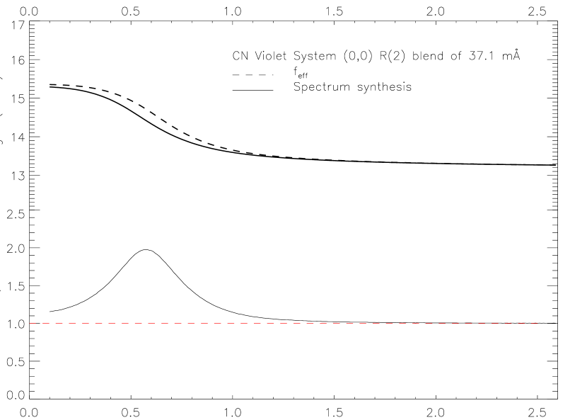
Figure 3: A comparison of the derived column density of the $N^{\prime\prime}=2$ level from the CN Violet System (0,0) R(2) line at 3873.37 Å. The solid line is obtained from the spectrum synthesis method, while the dashed line uses the effective oscillator strength and a curve of growth for a single, unblended line. The separation between the two principal lines of the blend is 0.54 km s^-1.

A correct treatment of the overlap of spectral lines in a blend necessarily requires the computation of synthetic spectra. A computer program (MOLLEY-CN) was developed that computes wavenumbers, Hönl-London factors and oscillator strength for any (isotopic) band of the CN Red and Violet System. From these numbers a synthetic spectrum based on a Voigt profile is computed. Input to the program is the rotational temperature, total column density, isotope ratios, Doppler $b$-parameter, and the spectral resolution of the output spectrum. MOLLEY-CN is available on request from the authors. As an aid to those who prefer the method of effective oscillator strength, we have investigated the error this latter method introduces on the derived column densities. For this purpose we have chosen the CN Violet (0,0) R(2) blend for which the two principal transitions are separated by 0.54 km s^-1. For a range of Doppler $b$-parameters the column density of the $N^{\prime\prime}=2$ (F₁ and F₂) level has been computed using the effective oscillator strength and synthetic spectra for a line with an equivalent width of 37.1 mÅ. Fig. 3 demonstrates the results. The derived $b$-parameter in this work is $b=0.51\pm 0.04$ km s^-1, and the effective oscillator strength method is clearly unacceptable for this work. We therefore will use the method of computing synthetic spectra to determine the column density responsible for the observed equivalent width of a “blend”. The only remaining limitation is that the line might be blended with transitions originating from other $N^{\prime\prime}$ level and that the rotational temperature must be given to compute such a blend. This limitation is easily overcome by iteration using an improved estimate of the rotational temperature.

Fig. 3 can be qualitatively understood in the following way. Use of $f_{\rm eff}$ assumes that the lines which form a blend (R(2) is a triplet) have exactly the same wavelength. This approximation is valid only for $b$-values much larger than the separation between the lines of a blend. Fig. 3 demonstrates this as the computed column density from the two methods are the same for large $b$-values. For small $b$-values, the use of $f_{\rm eff}$ fails because the lines are (partly) separated and the blend absorbs more efficiently than assumed by the $f_{\rm eff}$ method. For a given equivalent width of a line, this means that the spectrum synthesis method yields a lower column density than the $f_{\rm eff}$ method. The R(2) blend has three lines. For moderate column densities, the contribution of the weakest line (^RQ₂₁ (2)) can be neglected and the ratio of the column density as derived from the two method is given by the inverse of the slope of the curve of growth. The slopes are: 1 for the linear part, 0.5 for the damping wings, and $<$ 0.5 for the saturated part of the curve of growth, and the maximum ratios are therefore: 1, 2 and $>$ 2. We see that in Fig. 3 the ratio goes to 2 when the two strongest lines of the triplet are on the saturated part of the curve of growth, For larger column densities, the blend is highly saturated and the broad damping wings contribute significantly to the equivalent width. The damping wings will be the same in both cases and the ratio will go to one. We note that in the “real” world lines never become this strong.

4 Analysis

4.1 Velocities

From the molecular lines with tabulated laboratory wavenumbers, we find an average heliocentric radial velocity of $77.5\pm 0.5$ km s^-1. To within the errors of the measurements, the velocity is independent of the rotational level $N^{\prime\prime}$. All velocities given in this article are corrected to the heliocentric rest frame. HD 56126 is a pulsating star (Oudmaijer & Bakker 1994, Lèbre et al. 1996, discussion of Paper II) and the photospheric velocity derived from our spectra will not be a good estimate of the systemic velocity of the star. In order to derive an expansion velocity we use the systemic velocity derived from CO radio line emission (for overview see Paper I). For $v_{\ast,CO}=85.6\pm 0.5$ km s^-1  we arrive at an expansion velocity of $v_{\rm exp}=8.1\pm 0.7$ km s^-1. This result is consistent with that derived from the width of the CO lines: $v_{\rm exp}=12.1\pm 1.0$ km s^-1 (Nyman et al. 1992). The expansion velocity is similar to expansion velocities of AGB stars suggesting that the molecule-containing layer around the post-AGB star, which is possibly part of the terminal “superwind” of the AGB star, was not ejected at very high velocity (panel b of Fig. 3).

4.2 Doppler $b$-parameter and synthetic spectra

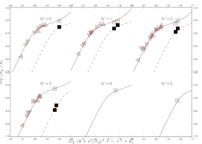
Figure 4: Curve of growth for each $N^{\prime\prime}$ level. The displacement of CN (solid line) and ¹³CN (dashed line) along the horizontal axis gives the isotope ratio derived from that $N^{\prime\prime}$ level. Squares for the Violet System (0,0), and triangles for the Red System bands (triangle pointing up (1,0), right (2,0), down (3,0), and left (4,0)). The over plotted theoretical model is for $b=0.51$ km s^-1.

In paper I it was demonstrated that the Red System (3,0) band is just saturated while the stronger (2,0) and (1,0) are saturated. From this it is obvious that the Violet System (0-0) band with $f_{\rm V}$-values a factor of ten higher than the Red System must be highly saturated. Of course, this circumstance facilitates the detection of the ¹³CN lines. The degree of saturation can be judged from Fig. 4 showing curves of growth for each $N^{\prime\prime}$ level. Observed lines from a given $N^{\prime\prime}$ level are combined into a single curve using the adopted $f$-values. The fitted theoretical curve is computed from a single line assuming $b=0.51$ km s^-1. Clearly the unsaturated lines are all from the Red System: 3-0 and 4-0 for the $N^{\prime\prime}=0$ level, but extending to the 1-0 band for the $N^{\prime\prime}=3$ level. For all relevant $N^{\prime\prime}$ levels, the ¹²CN/¹³CN ratio is obtainable from a comparison of ¹³CN Violet System lines with CN Red System lines of about the same strength. Thus, the ¹²CN/¹³CN ratio is insensitive to the $b$-value but dependent on the ratio of the $f$-values for the Violet and Red System. A sensitivity to the $b$-value does exist because, as noted above, the precise curve of growth is dependent on the make-up of individual CN features. For a detailed analysis we must determine the Doppler $b$-parameter and derive column densities from the observed equivalent widths by taking into account the details of the blends and optical depth effects.

For each transition (spectral line) there are two unknown parameters which affect the observed equivalent width: the Doppler $b$-parameter and the column density of the level the transition originates from ($N(N^{\prime\prime}$)). The $b$-parameter must be the same for all lines, under the assumption that they are all formed from the same gas. The $N(N^{\prime\prime})$ is the same for those transitions for a given level $N^{\prime\prime}$ of the same isotope. In this study we included $N^{\prime\prime}=0,1,2,3,4,5$ for CN and $N^{\prime\prime}=0,1,2,3$ for ¹³CN, thus ten independent column densities. We assumed that the F₁ and F₂ level population is given by their degeneracy level and the energy of the average $N^{\prime\prime}$ level. We solved for $b$ and $N(N^{\prime\prime})$ in the following manner:
For a range of $b$-parameters ($0.10\leq b\leq 2.60$ km s^-1  in steps of 0.01 km s^-1), the column density responsible for the observed equivalent width of the blend is determined by means of spectrum synthesis. We did not fit the observed spectra directly, but instead used the observed equivalent width. Although we have ten independent measure of the $b$-parameter, most of the $N^{\prime\prime}$ levels are only probed by one or two lines and the errors are rather large. We have limited the analysis therefore to the CN $N^{\prime\prime}=0,1,2,3$ levels which are each probed by at least ten blends. For each $b$-parameter, $\log N(N^{\prime\prime})$ and its standard deviation where computed. The final $b$-parameter is given by the combination for which the standard deviation is minimal, and by averaging the $b$-parameter weighted by the number of lines. The CN Doppler-parameter was found to be $b=0.51\pm 0.04$ km s^-1. This same process was repeated for C₂ using the data of Paper I, and this resulted in $b=0.53\pm 0.03$ km s^-1. Since the CN data is of higher quality we adopt $b=0.51\pm 0.04$ km s^-1  for both CN and C₂. Given the $b$ value, the $FWHM$ of the absorption line profile should be at least $0.85\pm 0.05$ km s^-1. In order to resolve these lines a spectral resolution of $R\geq 350,000$ is needed. This confirms that we are not be able to resolve these lines profiles in our spectra. The line profiles of the synthetic spectra can be perfectly fitted to the observed ones for this $b$-value convolved to the spectral resolution of the observations. No additional macroturbulent broadening is needed to explain the observations.

4.3 Column densities and rotational temperatures

Some additional lines were observed which are identified as due to perturbations (Prasad et al. 1992). Perturbations occur from the crossing of energy levels in two different electronic manifolds (Kotlar et al. 1980). The perturbations in the Violet System (0,0) band originate from B${}^{2}\Sigma$ $v=0$ levels perturbed by the A${}^{2}\Pi$ $v=10$ level. Perturbations affect the oscillator strength of lines. Since a study of the perturbations is beyond the scope of this work, we will not include the perturbed lines in our analysis.

The derived average column density per $N^{\prime\prime}$ level and isotope is listed in Table 4. Given these column densities an absolute rotational diagram can be constructed (Fig. 5) and the rotational temperature can be determined. Using a first order fit (constant $T_{\rm rot}$), we find $T_{\rm rot}($CN$)=12.8\pm 0.6$ K, and $T_{\rm rot}(^{13}$CN$)=8.0\pm 0.6$ K. The rotational temperature for $N^{\prime\prime}=0,1,2$ and 3 of CN is determined very largely by the weak CN Red System lines, especially the (3-0) and (4-0) lines measured off our McDonald spectra: $T_{\rm rot}($CN$)=11.1\pm 0.8$ K. For $N^{\prime\prime}=4$ and 5, the column density is set almost exclusively by a CN Violet System line which, in the case of $N^{\prime\prime}=4$, is partially saturated: the $N^{\prime\prime}=4$ and 5 levels give a temperature of ($T_{\rm rot}($CN$)=10.8\pm 0.8$ K) that within the errors is identical to the temperature from $N^{\prime\prime}=0$ to 3. The column density for $N^{\prime\prime}=4$ and 5 seems higher by 0.3 dex than given by extrapolation from $N^{\prime\prime}=0$ to 3. This offset corresponding to a reduction of the Red System $f_{\rm R}$-values by a factor two (relative to the Violet System) is probably excluded by experimental and theoretical results on the $f$-values (see above). A single rotational temperature (Table 4) can be fitted to the points in Fig. 5.

Available ¹³CN lines, all from the Violet System, are partially saturated except for the $N^{\prime\prime}=3$ lines. Saturation means that the derived column densities are dependent on the $b$-value and the adopted splitting of the unresolved lines that make up the lines. In light of the fact that the $b$-values from CN and C₂ are in excellent agreement, we believe the $b$-value is not a serious contributor of uncertainty to the determination of $T_{\rm rot}$ for ¹³CN. Certainly, the column density of $N^{\prime\prime}=0$ cannot be lowered (relative to $N^{\prime\prime}=3$) by 0.5 dex needed to make the ¹³CN rotational temperature equal to that of CN.

From a study of millimeter emission lines (e.g. CO and CN) of seven planetary nebulae, Bachiller et al. (1997b) found a kinetic temperature of the CN line forming region of only 25 K, and a rotational temperature of CN of 5-10 K. Quite unexpectedly we found different rotational temperatures for CN and ¹³CN of $T_{\rm rot}=11.5\pm 0.6$ and $8.0\pm 0.6$ K respectively.

In light of the continuing discrepancies between experimental and theoretical estimates for the CN Red System’s $f_{\rm R}$-values and the radiative lifetimes of the A${}^{2}\Pi$ state, it is of interest to consider if our spectra can give useful information on the ratio ($f_{\rm R}/f_{\rm V}$) of the Red to Violet System $f$-values. Of course, the fundamental problem is that the Violet strongest lines of a given $N^{\prime\prime}$ are much stronger than the strongest Red System lines of the same $N^{\prime\prime}$ (¹³CN lines are of comparable strength to the Red System CN lines but the ¹²CN/¹³CN ratio is not independently known). A simple check of the $f_{\rm R}/f_{\rm V}$ is possible by insisting that each band yields the same column density. We have conducted this exercise and found that relative to the Violet System (0,0) band, the Red System bands give a larger total column density by a factor 2.3 (1-0), 2.4 (2-0), 2.1 (3-0), and 2.0 (4-0). To get consistent column densities the $f_{\rm R}$ values have to be decreased by this factor. This is clearly unacceptable and we will adopt our initial estimated of the $f$-values to proceed with our analysis. It seems that the correction factor is wavelength dependent: it increases with increasing wavelength. This could suggest that there is scattered light (continuum, or CN emission line radiation) which fills in the absorption profile. Since our observations were collected over several years (the Red System was mainly observed in 1992 and the Violet System only in 1997), there is the possibility that the strength of the lines have decreased with time. This idea can easily be tested by simultaneously observing both systems.

4.4 CN/¹³CN/¹⁴CN/C¹⁵N isotope ratios

Based on our findings of a different rotational temperature for CN and ¹³CN, it is clear that the CN/¹³CN ratio will dependent on the $N^{\prime\prime}$ levels included in the determination of the column densities. The CN/¹³CN ratio for each N^′′ level is given in Table 4 with an estimate of its uncertainty. In order to determine the isotope ratio of the line forming region we add the contributions from all $N^{\prime\prime}$ levels: CN/¹³CN = $\sum_{N^{\prime\prime}=0}^{5}N(N^{\prime\prime})^{\rm CN}/\sum_{N^{\prime\prime}=0}^{3}N(N^{\prime\prime})^{\rm{}^{13}CN}=38.0\pm 1.5$. If the measured $T_{\rm rot}$ is applicable to $N^{\prime\prime}\geq 5$ levels, these bands contribute insignificantly to the summation.

Upper limits to the equivalent widths of 1.5 mÅ  for both the ¹⁴CN and C¹⁵N lines correspond to the following lower limits: CN/C¹⁵N($N^{\prime\prime}=1$) $\geq 2000$, and CN/¹⁴CN($N^{\prime\prime}=1$) $\geq 2000$. Assuming that the rotational temperature of ¹⁴CN and C¹⁵N is equal to the one of CN, we find lower limits of CN/C¹⁵N $\geq 2000$, and CN/¹⁴CN $\geq 2000$.

Table 4: Column densities and the isotope ratios derived from spectrum synthesis for $b=0.51$ km s^-1, and the $f$-values given in Sect. 3.1 & 3.2.

$N^{\prime\prime}$ $\log N(N^{\prime\prime})$ [cm${}^{-2}]$ CN/¹³CN CN/¹⁴CN CN/¹⁵CN CN ¹³CN ¹⁴CN C¹⁵N 0 $14.80\pm 0.17$(10) $13.22\pm 0.10$(1) $38.3\pm 3.0$ 1 $15.05\pm 0.17$(12) $13.59\pm 0.10$(2) $\leq 11.72$ $\leq 11.72$ $28.8\pm 2.1$ $\geq 2000$ $\geq 2000$ 2 $14.85\pm 0.16$(17) $13.16\pm 0.10$(2) $48.2\pm 2.8$ 3 $14.39\pm 0.13$(11) $12.44\pm 0.10$(2) $89.2\pm 3.9$ 4 $13.78\pm 0.10$(01) $\leq 11.79$ 5 $12.70\pm 0.10$(01) 6 $\leq 11.79$ preferred ratios Total: $15.44\pm 0.06$(52) $13.86\pm 0.09$(7) $\leq 11.72$ $\leq 11.72$ $38.0\pm 1.5$ $\geq 2000$ $\geq 2000$ $T_{\rm rot}$ [K]: $11.5\pm 0.6$ $8.0\pm 0.6$ - numbers in brackets are the number of lines used to determine the average column density. - errors are the standard deviations on the average, if less than 4 lines, 0.10 was adopted.

Figure 5: Rotational diagram for CN and ¹³CN with the column densities of Table 4 ($b=0.51$ km s^-1). Note that the slope of the two curves are different. This translates in CN having a higher rotational temperature than ¹³CN.

5 Discussion

Doppler parameter of $b=0.51\pm 0.04$ km s^-1  sets and upper limit on the kinetic temperature of $T_{\rm kin}=400\pm 50$ K. This is rather high for gas which is about $10^{16}$ cm from the central star (Meixner et al. 1997). Based on radio observations of CN towards post-AGB stars, Bachiller et al. (1997b) argue that they find $T_{\rm kin}\simeq 10{\rm~{}to~{}}25$ K. The $b$-parameter must, therefore, have an additional contribution from turbulence. The CN rotational temperature cannot be used to estimated the kinetic temperature since the molecule is sub-thermal. C₂ behaves supra-thermal, but the rotational temperature derive from the $J^{\prime\prime}=0$ and $J^{\prime\prime}=1$ level is a good indicator for the gas kinetic temperature. This would suggest $T_{\rm kin}\simeq 189$ K (Bakker & Lambert 1997). This value is also much higher than would be expected, and it is clear that we need an independent accurate determination of the kinetic temperature. The turbulence required is in the range of $v_{\rm micro}=0.36{\rm~{}to~{}}0.50$ km s^-1  and depends on the adopted $T_{\rm kin}$. The source of turbulence is not identified, but might be the result of small scale turbulence, non-Maxwellian velocity distribution, velocity stratification, the presence of multiple unresolved absorption components due to separate clumps.

An isotopic ratio as determined from molecules (${}^{i}{\rm XY}$ and ${}^{j}{\rm XY}$) does not necessarily reflect the intrinsic isotopic ratio (${}^{i}{\rm X}/^{j}{X}$) of the gas. For example, interstellar (and probably circumstellar) CO is subject to two competing processes which affect this ratio: photodissociation by line radiation and ion-molecule charge exchange (Watson et al. 1976). The net result depends on the local conditions (density, temperature, and radiation field).

Since photodissociation for the CO molecule is driven by line radiation, the more abundant CO, the more the molecule can shield itself against the dissociating by photons. The CN molecule is photodissociated by continuum radiation, not by lines. The ion-molecule reaction on the other hand will operate for CN. The gas-phase ion-molecule reaction for CN is given by:

$${\rm{}^{13}C^{+}}+{\rm{}^{12}CN}\rightleftharpoons{\rm{}^{12}C^{+}}+{\rm{}^{13}CN}+\Delta E$$ (1)

where $\Delta E$ is the zero-point energy difference derived from the molecular parameters (Prasad et al. 1992) and the relation of isotopic dependence of the Dunham coefficients. We find 31, 58, and 23 K for ¹³CN, ¹⁴CN, and C¹⁵N respectively. The reaction to the right will be referred to as the forward reaction ($k_{f}$) and to the left as the reverse reaction ($k_{r}$). C⁺ can be produced by cosmic ray ionization of free carbon atoms and molecules containing carbon (e.g. CO), and by the reactions of He⁺ with these molecules (where CO is the dominant one).

Our picture of the chemistry of the CN molecule in the circumstellar shell is a simple one. CN molecules which are produced by photodissociation of the parent molecule HCN, are subsequently destroyed by photodissociation. Between their formation and destruction, CN molecules participate in the isotopic exchange reaction. If the time scale for the isotopic exchange reaction is shorter than the lifetime of CN, then the exchange reaction will reach equilibrium:

$$R_{\rm eq}=R_{0}/\alpha$$ (2)

$${\rm with}$$

$$\alpha=\frac{k_{f}}{k_{r}}=e^{\Delta E/kT_{\rm kin}}$$ (3)

$$R_{0}=\frac{[^{12}{\rm C}^{+}]}{[^{13}{\rm C}^{+}]}=\frac{[^{12}{\rm C}]}{[^{13}{\rm C}]}$$ (4)

$$R_{\rm eq}=\frac{[^{12}\rm CN]}{[^{13}\rm CN]}$$ (5)

with the square bracket denoting the local density of that species in cm^-3, $R_{\rm eq}$ and $R_{0}$ the equilibrium CN and true C isotope ratio. A lower limit to the kinetic temperature is given by the CN rotational temperature of 12 K. This gives an upper limit on $\alpha$ of 13. For higher temperature, $\alpha$ decreases to unity. This clearly indicates that if the ion-molecule reaction is in equilibrium, we may underestimate the isotope ratio by as much as a factor 13! For a more realistic $T_{\rm kin}\simeq 25$ K, and an $R_{\rm eq}=23$, we find a true $R_{0}={\rm C}/^{13}{\rm C}=80$.

To assess the behavior of the ratio $\rm{}^{12}CN/^{13}CN$ in an expanding shell, we use the theoretical work of Cherchneff et al. (1993) on the chemistry of the circumstellar shell surrounding the carbon star IRC +10216. The shell radius where CN is more abundant than half its peak abundance are between $0.7\times 10^{17}$ and $1.3\times 10^{17}$ cm. Together with the expansion velocity this gives a lifetime for CN of about $2\times 10^{3}$ years. Basically this is the lifetime of a single CN molecule after photodissociation of HCN, before the photodestruction of CN, not taking into account any other reaction that could produce or destroy CN.

The time scale for the ion-molecule reaction is more difficult to estimate. Adams et al. (1985) computed reaction rates ($k_{f}$) for polar molecules and found that they are as high as $10^{-7}$ cm³ s^-1 for low temperature gas ($T_{\rm kin}<50$ K). The radius at which the CN abundance peaks ($r\simeq 1.0\times 10^{17}$ cm^-3) has a C⁺ abundance of $3\times 10^{-4}$ cm^-3. The time scale for the isotopic exchange reaction as derived from the forward rate coefficient and this C⁺ particle density is of the order of $1\times 10^{3}$ years. The isotopic exchange reaction time scale is comparable to the CN life time. This suggest that we have to look into this process in some greater detail.

Figure 6: (a) The density of CN and ¹³CN (solid lines) and C⁺ and ¹³C⁺ (dashed lines) as function of distance to the star (adopted from Cherchneff et al. 1993). (b) The contribution of the column density to the total column density, normalized to a peak value of 1. (c) The local isotope ratio for CN and C⁺ as function of radius for reaction rates of $\log k_{f}$=-11 to -3 in steps of 1. $k_{f}=1.0\times 10^{-7}$ is enhanced. (d) The final observed isotope ratio, with a dot at our preferred rate coefficient.

The effect of the isotopic exchange reaction should ideally be studied by computing self consistent chemical models for the abundances and radiation field appropriate for HD 56126. Such a study is beyond the scope of this work, instead we will make some estimates. A model of the circumstellar shell of the carbon star IRC +10216 has been computed by Cherchneff et al. (1993). This model uses a large number of chemical reactions, the interstellar radiation field, circumstellar reddening, and computes the abundances of the most important molecular species. The two major differences between IRC +10216 and HD 56126 are (i) the inner shell radius of HD 56126 will be much larger than for IRC +10216, and (ii) the radiation field of HD 56126 (7000 K, Klochkova 1995) is significantly hotter than that of IRC +10216 (3500 K). The larger inner radius does not affect the chemical structure of the remaining shell. A 7000 K stellar radiation field has fewer UV photons than the interstellar UV field (see Paper II) such that the interstellar radiation field will dominate the photodissociation processes. Therefore the chemical structure of IRC +10216 is applicable to HD 56126. From the model, we infer that CN is produced mainly by photodissociation of HCN and destroyed by photodissociation into C and N. From Cherchneff et al. we take the CN and C⁺ density (panel a of Fig. 6). Assuming that the isotopic exchange reaction for CN has reached equilibrium ($T_{\rm kin}=25$ K), we assume a true isotope ratio of $R_{0}=67$. From this we compute where the contribution to the observed column density comes from (panel b of Fig. 6): the line is formed where the CN density is highest. For a range of reaction rates we have computed the local CN and ¹³CN densities, while the C⁺ density in unaffected by the isotopic exchange reaction. (panel c of Fig. 6). C⁺ is mainly formed from CO and the processes involved in the production of C⁺ are not coupled to CN. The assumed reaction rate is $k_{f}=1.0\times 10^{-7}$. We see that the transition from the initial CN isotope ratio to the equilibrium value occurs where the CN density is highest and that this transition is rather fast. From these densities, we can computed the predicted observed CN isotope ratio (panel d of Fig. 6). To obtain an observed CN isotope ratio of 38 at $T_{\rm kin}=25$ K, we have to start with an intrinsic isotope ratio of $R_{0}=67$ and $R_{\rm eq}=19$. Clearly, the isotopic exchange reaction is important. Based on this analysis we suggest that the intrinsic carbon isotope ratio is ¹²C/¹³C=$67$ for $T_{\rm kin}=25$ K. Adams et al. (1985) show that the rate coefficient is dependent on the rotational quantum number. The higher the rotational quantum number, the lower the rate coefficient. If this dependence is rather strong, then the isotopic exchange reaction would be able to explain the difference in rotational temperature between CN and ¹³CN: for $N^{\prime\prime}=0$ more ¹³CN is formed than for $N^{\prime\prime}=5$ leading to a lower CN isotope ratio as derived from $N^{\prime\prime}=0$ than from $N^{\prime\prime}=4$.

Isotopic exchange reactions are very efficient at low temperatures and for high dipole moment molecules. From this we predict that CO (with a lower dipole moment) will be less affected, while C₂ with no dipole moment is unaffected. C₂ will therefore give the true isotope ratio and combined with CN this may give the kinetic temperature of the gas. The isotopic exchange reaction also enhances the abundance of ¹⁴CN and C¹⁵N.

In order to derive the mass-loss rate from the CN absorption lines we adopt the CN abundance (in number of particles) of $X_{\rm CN}=1.0\times 10^{-6}$ for AFGL 2688 (Bachiller et al. 1997a). AFGL 2688 (the Egg Nebula) is so far the only C2CN stars for which radio emission of CN has been observed. The inner and outer radius of the ejecta of HD 56126 have been determined by Meixner et al. (1997) by modeling the spatial distribution of the infrared source: $r_{\rm inner}=45\pm 2\times 10^{15}$ cm (1.0$\pm$0.15”), and $r_{\rm outer}=155\pm 15\times 10^{15}$ cm ($3.6\times 3.3^{\prime\prime}$ at 11.8 $\mu$m). Assuming that CN coincides with the infrared source, we find $\dot{M}=4.5\pm 0.8\times 10^{-5}$ M_⊙ yr^-1.

The prototype of the AGB stars, IRC +10216/CW Leo, is a massive, highly-evolved carbon star with $3M_{\odot}\leq M_{\rm ZAMS}\leq 5M_{\odot}$ (Guélin et al. 1995). For IRC +10216 the isotope ratios are well determined and give an estimate of the ratios which one might expect to detect for a carbon-rich post-AGB star like HD 56126: C/¹³C=44${}^{+3}_{-3}$, ¹²C/¹⁴C$\geq 62600$, N/¹⁵N$\geq$5300, O/¹⁷O=840${}^{+230}_{-170}$, and O/¹⁸O=1260${}^{+315}_{-240}$ (see Forestini & Charbonnel for an overview). Our estimate of the ¹²C/¹³C ratio for HD 56126’s shell is consistent with that of IRC +10216. Results for circumstellar shells around four other carbon stars were provided by Kahane et al. (1992): C/${}^{13}\leq 60$, $>30$, $32^{+10}_{-7}$ and $31^{+6}_{-5}$. These too suggest that HD 56126 is not exceptional.

A comparison may also be made with isotopic ratios pertaining to the photosphere of cool carbon (AGB) stars. It must be borne in mind that the photospheric ratios may evolve before the stars shed the material that becomes the circumstellar shell of a post-AGB star. Luminous AGB stars of intermediate mass experience H-burning at the base of their convective envelope. This decreases the C/¹³C ratio but rather quickly also converts the star from C-rich to O-rich. It seems improbable that C-rich post-AGB stars will have evolved from this intermediate stage. At lower luminosity and for lower mass stars, ¹²C from the He-burning shell is added following a thermal pulse. Repetition of this addition will increase the photosphere’s C/¹³C ratio unless H-burning converts ¹²C to ¹³C. On this scenario, the C/¹³C ratio of a post-AGB star might be higher than that of a typical AGB progenitor.

Through analysis of infrared spectra of N-type carbon stars, Lambert et al. (1986) showed that most stars had a C/¹³C ratio in the range 30 to 70: a value of 67 is not unusual. Ohnaka & Tsuji (1996), however, from analysis of spectra near 8000 Åreported, systematically lower ratios but a ratio of 67 would not be unusual, although on the high end of the distribution function. This possible shift between the C/¹³C ratio of stars and HD 56126 may be due to the fact that the stellar ratios continue to evolve before the post-AGB phase is reached. On the other hand, quantitative analysis of SiC circumstellar grains extracted from meteorites shows a C/¹³C distribution function that mimics well Lambert et al.’s stellar distribution, which suggests, perhaps, that evolutionary changes are minimal.

A priority goal has to be the determination of more accurate C/¹³C ratios for HD 56126 and an adequate sample of post-AGB stars. In the case of HD 56126 the ratio is presently uncertain for several reasons. A minor contributor to uncertainty is the combined use of CN Violet and Red System lines and the presence of uncertainty over the $f$-values of the Red System. This uncertainty could be avoided by re-observation of the strongest CN Red System bands to higher S/N ratio such that their ¹³CN lines are detectable. A key problem will remain in that the CN molecules are fractionated in the shell and this has to be modeled in order to extract the C/¹³C ratio that is of primary interest. This extraction requires a better understanding of physical conditions in the shell. We suggest that this understanding may be obtained by analyzing spectra of other C-containing molecules. In particular, C₂ is accessible by the Phillips system, and CO is probably detectable in the infrared. Lacking an electric dipole moment, the isotopic exchange reaction involving C₂ will be very slow, and, as we have already shown observationally (Bakker & Lambert 1997), the C₂ and CN rotational ladders are influenced differently by the local density and the ambient radiation field. The CO molecule has a smaller dipole moment than CN, and its photodissociation is line-dominated. Measurements of the ratios C₂/¹²C¹³C, and CO/¹³CO together with the CN/¹³CN ratio will shed light on the physical conditions in the shell, and on the true ¹²C/¹³C ratio. If such data can be assembled for a sample of post-AGB stars, it will be possible to trace a link with their AGB antecedents.

Appendix A Hönl-London factors and effective oscillator strength

Hönl-London factors were computed from the equations given in Schadee (1964) and Kovács (1969), and normalized according to the sum rule $\sum_{J^{\prime}}S_{J^{\prime}J^{\prime\prime}}=\left(2-\delta_{0,\Lambda^{\prime}+\Lambda^{\prime\prime}}\right)\times\left(2S^{\prime\prime}+1\right)\times\left(2J^{\prime\prime}+1\right)$ as stated by (Larsson 1983). For both the Red and Violet System we take $S^{\prime\prime}=0.5$ since both originate from the same ground level (${}^{2}\Sigma$). For the Red System ($\Pi-\Sigma$, $\Lambda^{\prime}=1$ and $\Lambda^{\prime\prime}=0$) we find $\delta_{0,1}=0$ and for the Violet System ($\Sigma-\Sigma$, $\Lambda^{\prime}=0$ and $\Lambda^{\prime\prime}=0$) $\delta_{0,0}=0$. For the Red System we summed over twelve transitions following the selection rule ($\Delta J=-1,0,1$ and $\Delta N=-2,-1,0,1,2$) (six for $N^{\prime\prime}=J^{\prime\prime}+0.5$ and six for $N^{\prime\prime}=J^{\prime\prime}-0.5$ for a given $J^{\prime\prime}$) ($\rm P_{1}$, $\rm Q_{1}$, $\rm R_{1}$, $\rm{}^{Q}P_{21}$, $\rm{}^{R}Q_{21}$, $\rm{}^{P}Q_{12}$, $\rm{}^{Q}R_{12}$, $\rm P_{2}$, $\rm Q_{2}$, $\rm R_{2}$, $\rm{}^{S}R_{21}$ and $\rm{}^{O}P_{12}$) and for the Violet System over six transitions following the selection rule ($\Delta J=-1,0,1$ and $\Delta N=-1,1$ ) (three for $N^{\prime\prime}=J^{\prime\prime}+0.5$ and three for $N^{\prime\prime}=J^{\prime\prime}-0.5$ for a given $J^{\prime\prime}$) ($\rm P_{1}$, $\rm R_{1}$, $\rm{}^{Q}P_{21}$, $\rm{}^{Q}R_{12}$, $\rm P_{2}$ and $\rm R_{2}$). For both the Red and Violet System this results in the relation: $\sum_{J^{\prime}}f_{J^{\prime}J^{\prime\prime}}=2\times f_{v^{\prime}v^{\prime\prime}}$. The oscillator strength of individual lines were checked against those of the SCAN tape (for the Red system) and those listed in literature (for the Violet system).

Given a Doppler broadening of $b=0.51$ km s^-1, transitions which are separated from each other by less than 0.012 Å  (Violet System), and 0.022 Å  (Red System), overlap and the two transitions should be treated as one line with an effective oscillator strength. Lines which are separated by more than this interval should be treated separately, although they might not be resolved in the spectrum. In physical terminology: if lines are separated by less than the Doppler $b$-parameters, their optical depth at any frequency point should be added before computing the line profile ($I=e^{-(\tau_{1}+\tau_{2})}$). If lines are separated by more than the Doppler $b$-parameter, the line profiles at any frequency point can be added ($I=0.5\times e^{-\tau_{1}}+0.5\times e^{-\tau_{2}}$), although adding the optical depth is also fine. For each blend we can determine an effective oscillator strength in the following way:

The F1 ($J^{\prime\prime}=N^{\prime\prime}+0.5$) and F2 ($J^{\prime\prime}=N^{\prime\prime}-0.5$) levels have different degeneracy:

$$g_{e}(F1)=2\times J^{\prime\prime}+1=2\times N^{\prime\prime}+2$$ (6)

$$g_{e}(F2)=2\times J^{\prime\prime}+1=2\times N^{\prime\prime}$$ (7)

Each $N^{\prime\prime}$ levels has therefore a degeneracy of

$$g_{e}(F1+F2)=2\times(2\times N^{\prime\prime}+1)$$ (8)

This is even valid for $N^{\prime\prime}=0$ although that level has no F2 levels. The reason for this is that each $J^{\prime\prime}$ level is split into $2\times J^{\prime\prime}+1$ so called $m$-levels. Those levels are only separated from each other under the influence of a strong external magnetic field (Zeeman splitting). In the case of circumstellar CN there is no observational evidence to assume that these levels are separated which indicates that there is no measurable magnetic field in the line forming region. To first order the $m$ levels for F1 and F2 for a given $N^{\prime\prime}$ have the same energy and therefore the same population. This allows us to write:

$$N(N^{\prime\prime},F1)=g_{e}(F1)/g_{e}(F1+F2)\times N(N^{\prime\prime},F1+F2)$$ (9)

$$N(N^{\prime\prime},F2)=g_{e}(F2)/g_{e}(F1+F2)\times N(N^{\prime\prime},F1+F2)$$ (10)

$$N(N^{\prime\prime},F1+F2)=N(N^{\prime\prime},F1)+N(N^{\prime\prime},F2)$$ (11)

$${\rm and}$$

$$f_{\rm eff}N(N^{\prime\prime})=\sum_{i}f_{i}N_{i}(N^{\prime\prime})$$ (12)

$$f_{\rm eff}N(N^{\prime\prime})=\left(\sum_{i}f_{i}(F1)\times(N^{\prime\prime}+1)+\sum_{i}f_{i}(F2)\times N^{\prime\prime}\right)\times\frac{N(N^{\prime\prime})}{(2\times N^{\prime\prime}+1)}$$ (13)

As examples we take two blends. $\Delta N=N^{\prime}-N^{\prime\prime}=0$ at 6194.5 Å  (Red System):

$$f_{\rm eff}N(N^{\prime\prime}=1)=\left(0.091\times 2+0.363\times 1\right)\times\frac{N(N^{\prime\prime}=1)}{3}=0.182N(N^{\prime\prime}=1)$$

and $\Delta N=N^{\prime}-N^{\prime\prime}=-1$ at 3876.3 Å  (Violet System):

$$f_{\rm eff}N(N^{\prime\prime}=2)=\left(0.0132\times 3+0.0022\times 2+0.0110\times 2\right)\times\frac{N(N^{\prime\prime}=2)}{5}=0.0132N(N^{\prime\prime}=2)$$

Appendix B Extra line lists

Table 5: Index of refraction for air. Table will not appear in journal.

Band	nair
Violet System (0,0)	1.000283
Red System (1,0)	1.000274
Red System (2,0)	1.000275
Red System (3,0)	1.000276
Red System (4,0)	1.000277

Table 6: CN Red System (1,0) with $f_{(1,0)}=1.90\times 10^{-4}$. Derived column densities are given in Table 4. Table will not appear in journal.

$B(N^{\prime\prime})$ $\lambda_{\rm rest}$ [Å] $f_{N^{\prime}J^{\prime},N^{\prime\prime}J^{\prime\prime}}\times 10^{4}$ $f_{\rm eff}\times 10^{4}N(N^{\prime\prime})$ [cm^-2] $W_{\lambda}$ [mÅ] Remark $\rm{}^{S}R_{21}$(3) 9129.142c 1.75 1.00N(3) no $\rm{}^{S}R_{21}$(2) 9133.730c 1.95 1.17N(2) no $\rm{}^{S}R_{21}$(1) 9136.579c 2.19 1.46N(1) no $\rm{}^{S}R_{21}$(0) 9139.686c 2.62 2.62N(0) 33.7 $\rm R_{2}$(3) 9141.169c 3.55 $\rm{}^{R}Q_{21}$(3) 9141.189c 3.77 3.67N(3) 35.3 $\rm R_{2}$(2) 9141.870c 3.55 $\rm{}^{R}Q_{21}$(2) 9141.886c 4.11 3.89N(2) 57.8 $\rm R_{2}$(1) 9142.828c 3.76 $\rm{}^{R}Q_{21}$(1) 9142.838c 4.62 4.33N(1) 57.8 polluted $\rm{}^{R}Q_{21}$(0) 9144.042c 6.34 6.34N(0) 57.8 $\rm Q_{2}$(1) 9147.208c 6.34 3.18N(1) 61.5 $\rm{}^{Q}P_{21}$(1) 9147.217c 1.60 $\rm Q_{2}$(2) 9149.167c 5.53 3.29N(2) 47.0 $\rm{}^{Q}P_{21}$(2) 9149.182c 1.79 $\rm Q_{2}$(3) 9151.381c 5.67 3.45N(3) 31.1 $\rm{}^{Q}P_{21}$(3) 9151.401c 1.79 $\rm P_{2}$(2) 9153.532c 1.59 0.636N(2) 27.4 $\rm P_{2}$(3) 9158.658c 2.02 0.866N(3) $\rm R_{1}$(3) 9177.032c 4.86 2.78N(3) 31.5 $\rm R_{1}$(2) 9179.911c 5.32 3.19N(2) 47.6 $\rm R_{1}$(1) 9183.209c 6.38 4.25N(1) 101.8 polluted $\rm R_{1}$(0) 9186.932c 10.10 10.10N(0) 59.9 $\rm{}^{Q}R_{12}$(3) 9189.465c 3.72 $\rm Q_{1}$(3) 9189.486c 5.61 97.8 polluted $\rm{}^{Q}R_{12}$(2) 9189.581c 5.03 $\rm Q_{2}$(2) 9189.597c 5.14 $\rm{}^{Q}R_{12}$(1) 9190.120c 8.96 5.83N(1) 62.9 $\rm Q_{1}$(1) 9190.129c 4.26 $\rm{}^{P}Q_{12}$(2) 9196.511c 3.38 1.802N(2) 42.2 $\rm P_{1}$(2) 9196.525c 0.75 $\rm{}^{P}Q_{12}$(3) 9199.171c 3.59 2.26N(3) 22.2 $\rm P_{1}$(3) 9199.192c 1.27 $\rm{}^{O}P_{12}$(3) 9206.114c 0.52 0.223N(3) no no: not observed thus not available

Table 7: CN Red System (2,0) with $f_{(2,0)}=9.03\times 10^{-4}$. Derived column densities are given in Table 4. Table will not appear in journal.

$B(N^{\prime\prime})$ $\lambda_{\rm rest}$ [Å] $f_{N^{\prime}J^{\prime},N^{\prime\prime}J^{\prime\prime}}\times 10^{4}$ $f_{\rm eff}\times 10^{4}N(N^{\prime\prime})$ [cm^-2] $W_{\lambda}$ [mÅ] Remark $\rm{}^{S}R_{21}$(0) 7871.654c 1.24 1.24N(0) 29.4 polluted $\rm R_{2}$(3) 7872.889c 1.68 $\rm{}^{R}Q_{21}$(3) 7872.905c 1.79 1.74N(3) 18.5 polluted $\rm R_{2}$(2) 7873.332c 1.68 $\rm{}^{R}Q_{21}$(2) 7873.343c 1.96 1.85N(2) 38.8 polluted $\rm R_{2}$(1) 7873.985c 1.79 $\rm{}^{R}Q_{21}$(1) 7873.992c 2.19 2.06N(1) 45.8 polluted $\rm{}^{R}Q_{21}$(0) 7874.852c 3.01 3.01N(0) 39.1 $\rm Q_{2}$(1) 7877.198c 3.01 1.51N(1) 98.2 polluted $\rm{}^{Q}P_{21}$(1) 7877.205c 0.76 $\rm Q_{2}$(2) 7878.686c 2.62 1.56N(2) 35.6 $\rm{}^{Q}P_{21}$(2) 7878.697c 0.85 $\rm Q_{2}$(3) 7880.384c 2.69 1.43N(3) 19.2 $\rm{}^{Q}P_{21}$(3) 7880.400c 0.85 $\rm P_{2}$(2) 7881.889c 0.76 0.30N(2) nd $\rm P_{2}$(3) 7885.725c 0.96 0.41N(3) nd $\rm R_{1}$(3) 7899.481c 2.31 1.35N(3) 42.0 polluted $\rm R_{1}$(2) 7901.520c 2.52 1.51N(2) 31.6 $\rm R_{1}$(1) 7903.892c 3.03 2.02N(1) 41.3 $\rm R_{1}$(0) 7906.598c 4.79 4.79N(0) 46.3 $\rm{}^{Q}R_{12}$(3) 7908.597c 1.76 $\rm{}^{Q}R_{12}$(2) 7908.611c 2.39 50.1 polluted $\rm Q_{1}$(3) 7908.613c 2.66 $\rm Q_{1}$(2) 7908.622c 2.43 $\rm{}^{Q}R_{12}$(1) 7908.959c 4.25 2.76N(1) 53.3 polluted $\rm Q_{1}$(1) 7908.966c 2.02 $\rm{}^{P}Q_{12}$(2) 7913.692c 1.60 0.86N(2) 19.1 $\rm P_{1}$(2) 7913.704c 0.36 $\rm{}^{P}Q_{12}$(3) 7915.714c 1.70 1.08N(3) 18.5 $\rm P_{1}$(3) 7915.729c 0.61 $\rm{}^{O}P_{12}$(3) 7920.804c 0.25 0.11N(3) nd no: not observed thus not available

Table 8: CN Red System (3,0) with $f_{(3,0)}=3.34\times 10^{-4}$. Derived column densities are given in Table 4. Table will not appear in journal.

B($N^{\prime\prime}$) $\lambda_{\rm rest}$[Å] $f_{N^{\prime}J^{\prime},N^{\prime\prime}J^{\prime\prime}}\times 10^{4}$ $f_{\rm eff}\times 10^{4}N(N^{\prime\prime})$ [cm^-2] $W_{\lambda}$[mÅ] Remark ${}^{S}R_{21}$(4) 6916.868l 0.282 0.157N(4) no ${}^{S}R_{21}$(3) 6918.581l 0.310 0.177N(3) no ${}^{S}R_{21}$(2) 6920.480l 0.343 0.206N(2) no ${}^{S}R_{21}$(1) 6922.568l 0.387 0.258N(1) no ${}^{S}R_{21}$(0) 6924.827l 0.461 0.461N(0) $10.7\pm 1.0$ $R_{2}$(4) 6925.811c 0.627 ${}^{R}Q_{21}$(4) 6925.821l 0.612 0.619N(4) $1.9\pm 0.5$ tentative $R_{2}$(3) 6925.893c 0.619 ${}^{R}Q_{21}$(3) 6925.909l 0.663 0.644N(3) $6.5\pm 0.5$ $R_{2}$(2) 6926.194c 0.622 ${}^{R}Q_{21}$(2) 6926.178l 0.725 0.684N(2) $16.3\pm 0.5$ $R_{2}$(1) 6926.656c 0.658 ${}^{R}Q_{21}$(1) 6926.650l 0.811 0.760N(1) $23.0\pm 0.5$ ${}^{R}Q_{21}$(0) 6927.304l 1.110 1.110N(0) $48.9\pm 5.0$ polluted $Q_{2}$(1) 6929.062l 1.110 0.555N(1) $18.8\pm 0.5$ ${}^{Q}P_{21}$(1) 6929.067c 0.278 $Q_{2}$(2) 6930.272l 0.969 0.576N(2) $14.0\pm 0.5$ ${}^{Q}P_{21}$(2) 6930.302c 0.314 $Q_{2}$(3) 6931.673l 0.992 0.605N(3) $6.0\pm 1.0$ line too weak ${}^{Q}P_{21}$(3) 6931.663c 0.315 $P_{2}$(2) 6932.715l 0.278 0.111N(2) $6.0\pm 0.5$ $Q_{2}$(4) 6933.179l 1.030 0.627N(4) $\leq 1.5$ ${}^{Q}P_{21}$(4) 6933.206c 0.305 $P_{2}$(3) 6935.720l 0.353 0.151N(3) $\leq 1.5$ $P_{2}$(4) 6938.910l 0.399 0.177N(4) $\leq 1.5$ $R_{1}$(4) 6945.273l 0.811 0.451N(4) $\leq 1.5$ $R_{1}$(3) 6946.479l 0.850 0.486N(3) $5.9\pm 1.0$ $R_{1}$(2) 6947.962l 0.929 0.557N(2) $13.0\pm 0.5$ polluted $R_{1}$(1) 6949.763l 1.115 0.743N(1) $24.0\pm 1.0$ $R_{1}$(0) 6951.816l 1.766 1.766N(0) $24.0\pm 5.0$ ${}^{Q}R_{12}$(2) 6953.415c 0.881 $Q_{1}$(2) 6953.461l 0.898 $24.1\pm 0.5$ ${}^{Q}R_{12}$(3) 6953.459c 0.655 $Q_{1}$(3) 6953.461l 0.980 ${}^{Q}R_{12}$(1) 6953.643c 1.568 1.021N(1) $25.7\pm 0.5$ $Q_{1}$(1) 6953.643l 0.747 ${}^{Q}R_{12}$(4) 6953.776c 0.532 $Q_{1}$(4) 6953.787l 1.040 0.814N(4) $2.3\pm 0.5$ tentative ${}^{P}Q_{12}$(2) 6957.302c 0.593 0.316N(2) $8.4\pm 0.5$ $P_{1}$(2) 6957.301l 0.132 ${}^{P}Q_{12}$(3) 6958.905c 0.631 0.397N(3) $4.6\pm 0.5$ $P_{1}$(3) 6958.907l 0.222 ${}^{P}Q_{12}$(4) 6960.782c 0.612 0.433N(4) $\leq 1.5$ $P_{1}$(4) 6960.805l 0.289 ${}^{O}P_{12}$(3) 6962.795l 0.092 0.039N(3) $\leq 1.5$ ${}^{O}P_{12}$(4) 6966.212l 0.138 0.061N(4) $\leq 1.5$ no: not observed thus not available