Global stability and the mass-to-light ratio of galactic disks

Abstract

We examine the global stability of an exponential stellar disk embedded in a dark matter halo and constrain the mass-to-light ratio of observed disks in the I-band, $\Upsilon_{I}$. Assuming only that the radial surface density distribution of disks is exponential, we derive an analytic upper limit: $\Upsilon_{I}\la 2.4h$, for a Hubble constant of $100h~{}\mbox{km s${}^{-1}$}\mbox{Mpc}^{-1}$. Using $N$-body simulations we derive a stability criterion significantly different from that of previous authors. Using this criterion we argue that, almost independent of the concentration of the halo, $\Upsilon_{I}\la 1.9h$. We discuss this result in relation to other independent determinations of $\Upsilon_{I}$, its limitations and its implications for theories of disk formation and barred galaxies.

1 Introduction

Stellar disks are a potentially powerful probe of the mass distribution in spiral galaxies. In particular, the rotation curve (defined in Section 2) is a direct probe of the gravitational force in the disk. The fact that the rotation curves of spiral galaxies are rather flat is usually taken to imply the presence of an extended halo of dark matter (e.g. Freeman 1970, Persic & Salucci 1991). Dark halos have been traditionally modelled by isothermal spheres with homogeneous cores, and assigned a mass-to-light ratio according to the ‘maximum-disk’ hypothesis, in which the largest mass possible is assigned to the disk consistent with the rotation curve (Carignan & Freeman 1985). Recent theoretical work has suggested that the isothermal form of the halo may not be appropriate (Navarro, Frenk & White 1996, Moore et al. 1997, Kravstov et al. 1997). Rix & Courteau (1997) have recently argued that the Tully-Fisher relation (Tully & Fisher 1977) has too little scatter to be consistent with the maximum-disk hypothesis.

Dalcanton, Spergel & Summers (1997), and Mo, Mao & White (1997) point up the need for a consistent and accurate picture of disk mass-to-light ratios for the theory of disk formation, and to understand the Tully-Fisher relation. As was pointed out by Rix & Courteau (1997), the maximum disk hypothesis and the Tully-Fisher relation are together incompatible with a near universal mass-to-light ratio, $\Upsilon$. Yet, the stellar populations of spiral disks at $z=0$ are generally believed to have rather uniform properties. In particular they all have similar colours, which leads one to believe that they should have similar $\Upsilon$.

Ostriker & Peebles (1973) argued that extended halos of dark matter in disk galaxies are required to stabilize the disks against global bar instabilities. They were able to draw very strong conclusions from $N$-body simulations with only 300 particles. Efstathiou, Lake & Negroponte (1982) (ELN) conducted larger $N$-body experiments specifically with disk components appropriate for real galaxies, and concluded that $\Upsilon_{\rm bol}\leq 1.5\pm 0.2$.

ELN compared their numerical results with only 12 galaxies due to limited data at that time. Since then, observations of spiral galaxies have improved tremendously owing to the great interest in the Tully-Fisher relation as a distance indicator (Giovanelli et al. 1997 and references therein). Large samples of spiral galaxies are now available (e.g. Mathewson & Ford 1996; Courteau 1996, 1997). In this paper, we re-examine the constraints from considerations of global stability which may be placed on the mass-to-light ratio of disks.

In the next section we review the properties of exponential disks, and their relation to real disk galaxies. In Section 3 we review the physics of global instability in disks. In Section 4 we describe the observations of disk galaxies, and how they can be used to constrain $\Upsilon$. In Section 5 we describe our $N$-body simulations. In Section 6 we discuss the results of independent determinations of mass-to-light ratios of galactic disks. In Section 7 we discuss the implications of our results and draw conclusions.

2 Exponential disks

The luminous disks of spiral galaxies are commonly modelled by an exponential surface brightness distribution:

$$\mu(R)={L_{\rm d}\over 2\pi R_{\rm d}^{2}}\exp(-R/R_{\rm d})$$ (1)

where $R$ is the usual cylindrical radius, and $L_{\rm d}$ is the total luminosity of the disk. Here we collect some notation and a number of useful results relating to exponential disks.

The disk has a mass $M_{\rm d}$, and a mass-to-light ratio in the $I$-band $\Upsilon_{I}$ in solar units. Thus the surface mass density of the disk is

$$\Sigma(R)=\mu(R)\Upsilon_{I}={M_{\rm d}\over 2\pi R_{\rm d}^{2}}\exp(-R/R_{\rm d}).$$ (2)

The gravitational potential in the disk $\Phi$ is conveniently decomposed into contributions from the disk and a halo:

$$\Phi=\Phi_{\rm d}+\Phi_{\rm h}.$$ (3)

(We use the subscripts ‘d’ for ‘disk’, and ‘h’ for ‘halo’ throughout.) We assume for the present purposes that the halo is spherical, and usually we think of it as being composed of dark matter, but it may also contain a stellar component (e.g. the ‘bulge’ of an earlier type spiral).

The speed of test particles on circular orbits $v_{\rm c}$ as a function of $R$ is given by

$$v^{2}_{\rm c}(R)=-{\partial\Phi\over\partial R}.$$ (4)

For the sake of definiteness, we shall refer to $v_{\rm c}(R)$ as the ‘true rotation curve’ of the system (or just ‘the rotation curve’). The observed line-of-sight velocity of a tracer population corrected for inclination we refer to as the rotation curve of the tracer. For instance, the HI rotation curve (apart from small contributions from turbulent motion) is thought to be a good measure of the true rotation curve as long as the system is axisymmetric. Some of the samples of galaxies used in this paper have rotation curves measured in H_α, but analyzed in a way which is supposed to maximize the agreement with HI (Raychaudhury et al 1997, Courteau 1997).

Following Efstathiou, Lake & Negroponte (1982) we define the dimensionless quantity

$$\epsilon_{\rm m}={v_{\rm m}\over(GM_{\rm d}/R_{\rm d})^{1/2}},$$ (5)

where $v_{\rm m}$ is the maximum value of $v_{\rm c}$, and $G$ is the gravitational constant. The rotation curve of an isolated exponential disk ($\Phi_{\rm h}=0$) is (Freeman 1970):

$$v^{2}_{\rm d}(R)={2GM_{\rm d}\over R_{\rm d}}y^{2}[I_{0}(y)K_{0}(y)-I_{1}(y)K_{1}(y)],$$ (6)

where $y=R/(2R_{\rm d})$. $I_{i}$ and $K_{i}$ are modified Bessel functions. An isolated disk has $\epsilon_{\rm m}\equiv\epsilon_{\rm d}\approx 0.63$ and a disk embedded in a halo has $\epsilon_{\rm m}>\epsilon_{\rm d}$.

3 Global stability

An isolated thin exponential disk is known to be violently unstable, as are all isolated thin disks. The fastest growing instability is generically global (the whole system is deformed) and bar shaped. The instability in conservative and/or collisionless systems is generally purely dynamical (growth timescale of order the crossing time). Secular instabilities set in in systems with dissipation and/or collisions generally on longer timescales. The disk may be stabilized if the disk is thickened in the vertical direction, as exemplified by the Maclaurin sequence of gaseous spheroids (Chandrasekhar 1969): near spherical members of the family are stable; they become first secularly and then dynamically unstable as the eccentricity is increased (see for example Christodoulou, Schlosman & Tohline 1995). A similar pattern is found for the stellar analogues of the Maclaurin spheroids. Stability may also be conferred by adding an external potential—in the extreme limit that the disk is composed of test particles it is trivially stable. As was pointed out by Ostriker & Peebles (1973) this mechanism can be used on rather general grounds to argue that spiral galaxies contain halos of dark matter.

There has been some debate as whether a disk with a given eccentricity and/or external potential is expected to be stable on theoretical grounds. Many attempts have been made to find a single parameter which delineates a boundary between stability and instability. Ostriker & Peebles (1973) used as a parameter the ratio

$$t_{\rm OP}=T_{\rm mean}/W$$ (7)

of the mean kinetic to total potential energy. The stellar disks studied by Ostriker & Peebles (1973) were stable if $t_{\rm OP}<0.14$ to very high accuracy. Remarkably, this criterion was shown to unify their results with all existing results on the stability of disks. Subsequent authors pointed to various insufficiencies of $t_{\rm OP}$ as applied to specific cases (Miller 1978, Miller & Smith 1979). Efstathiou, Lake & Negroponte (1982) refined the definition to patch up some of these difficulties, defining a related parameter $t_{*}$, but in the end concluded that $\epsilon_{\rm m}$ (cf. equation 5) was a better indicator of stability for their models. In particular they found that all models with $\epsilon_{\rm m}\la 1.1$ were unstable, whereas the stability boundary in $t_{*}$ depended on the halo concentration. Christodoulou, Schlosman & Tohline (1995) proposed a further refinement of $t_{*}$ by analogy with the Maclaurin series, defining a new parameter

$$\alpha=\sqrt{{\textstyle{1\over 2}}ft},$$ (8)

where $t=T/W$ and $f$ is a form factor dependent on the shape of the disk. Both $t$ and $f$ were given precise definitions only for the Maclaurin sequences. They showed that $\alpha$ led to a stability criterion which was broadly consistent with that of ELN. However, $\alpha$ was not defined properly for disks with external potentials, and they failed to address the issue of the halo concentration.

The importance of global stability is this: the disks in spiral galaxies appear to be long lived, and the majority do not contain bars. In the next section we describe how the apparent stability of galactic disks can be used to constrain their mass-to-light ratio.

$\epsilon_{l}h^{-{\textstyle{1\over 2}}}$

$\mu_{0}(I-\hbox{mag/sec}^{2})$

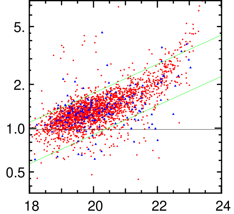
Figure 1: The quantity $\epsilon_{l}h^{-1/2}$ (as defined in equation 10) is shown versus $I$-band central surface brightness for the sample of spiral galaxies of Mathewson & Ford (1996) (with crude bulge correction, see text). On this plot, a fixed value of $\epsilon_{\rm m}$ corresponds to a horizontal line with amplitude $\epsilon_{\rm m}(\Upsilon_{I}h^{-1})^{1/2}$. The horizontal solid line shows the value of $\epsilon_{\rm m}$ for a self-gravitating disk ($\epsilon_{\rm m}=0.63$) with $\Upsilon_{I}=2.14h$. The two shaded lines bracket the predicted ranges (see text). Barred galaxies are shown as triangles.

4 Comparison with observations

To compare a theoretical instability criterion with observations, we need both detailed rotation curves (to obtain $v_{\rm m}$) and surface photometry (to obtain $R_{\rm d}$). We have examined the data from a wide variety of sources. The largest data set is that of Mathewson & Ford (1996) (MF) which has rotation velocities and $I$-band photometry for a sample of nearly 2500 Southern spiral galaxies taken from the ESO-Uppsala catalogue. The majority are relatively late types: of those 2275 for which Hubble types are given, 1055 are Sc or Sbc; 814 are Sb; and 5 are Sa. We convert the published photometric quantities to $R_{\rm d}$ and the central surface brightness $\mu_{0}$ by assuming an exponential profile. Details are given in an Appendix. The Appendix also describes how we make a crude bulge subtraction from the MF data, the results being labelled MFD in Table 1. Since Mathewson & Ford (1996) provide the largest uniform data set we adopt it whenever we quote a numerical result (including bulge subtraction when not explicitly specified). We list the other data sets for comparison purposes.

Table 1: Observational data and summary of limits on $\Upsilon_{I}$. Column (1), Name of data set; (2), number of galaxies; (3) median central surface brightness $\langle\mu_{0}\rangle$ in mag/sec²; (4), $\epsilon_{l}$ minimum, maximum, median and 10% quantile values; (5) $\Upsilon_{I}$ limit derived from 10% quantile and assuming $\epsilon_{\rm m}>0.63$; (6) assuming $\epsilon_{\rm m}>0.72$. See text for description of data set names. The row labelled ‘All’ contains the combined properties of all the preceding rows. MFB refers to the subset of MF which is barred.

Set	$N$	$\langle\mu_{0}\rangle$	$\epsilon_{l}$[min,max,med,10%]	$\Upsilon_{I}$(1)	$\Upsilon_{I}$(2)
MF	2446	$19.97$	$[0.43,7.50,1.19,0.92]$	$2.14$	$1.64$
C97	304	$20.14$	$[0.54,2.03,1.13,0.90]$	$2.02$	$1.55$
C96	316	$20.39$	$[0.76,1.84,1.15,0.96]$	$2.34$	$1.79$
SML	23	$22.87$	$[0.54,5.72,1.95,1.04]$	$2.72$	$2.08$
SMH	23	$20.97$	$[0.67,3.56,1.32,0.80]$	$1.62$	$1.24$
BBFN	371	$18.47$	$[0.35,2.10,0.99,0.70]$	$1.24$	$0.95$
DG	84	$20.05$	$[0.59,1.77,1.04,0.84]$	$1.79$	$1.37$
RBKG	25	$20.89$	$[0.89,1.78,1.28,1.08]$	$2.93$	$2.24$
B	12	$19.89$	$[0.67,1.96,1.12,0.84]$	$1.77$	$1.35$
All	3604	$20.01$	$[0.35,7.50,1.16,0.88]$	$1.96$	$1.50$
MFD	2446	$19.97$	$[0.45,7.50,1.30,0.98]$	$2.41$	$1.85$
MFB	175	$19.94$	$[0.54,4.37,1.20,0.90]$	$2.05$	$1.57$

The data of Courteau (1996) and Courteau (1997) are in principle the same, but one paper gives kinematic measurements and the other photometric, and we list them separately. To obtain the missing data in these cases we use the observed Tully-Fisher relation (Giovanelli et al. 1997; Shanks 1997):

$${\cal M}_{I}-5\log h=-(21.00\pm 0.02)-(7.68\pm 0.13)(\log W-2.5),$$ (9)

where $h$ is the Hubble constant in units of $100~{}\mbox{km s${}^{-1}$}\mbox{Mpc}$, and where $W$ is the inclination-corrected width of the HI line profile. The maximum of the rotation curve $v_{\rm m}$ is given by $v_{\rm m}=W/2$. Courteau (1997) has measured rotation not in HI, but in H_α. Raychaudhury et al. (1997) show that to a good approximation values of $W$ determined from H_α are consistent with those determined from HI.

For data sets without $I$-band quantities we convert using for all galaxies $B-I=1.7$ (de Jong 1996) and $r-I=0.77$ (Rix & Courteau 1997). When $R_{\rm d}$ or $\mu_{0}$ are missing we calculate them assuming an exponential profile.

The other data sources are as follows with a short description of the quantities provided. C97: ($R_{\rm d}$, $v_{\rm m}$) provided by the author from Courteau (1997). C96: Courteau (1996) ($R_{\rm d}$, $r$-magnitudes). SML: de Blok & McGaugh (1996) low surface brightness galaxies ($R_{\rm d}$, $v_{\rm m}$, $B$-magnitudes). SMH: de Blok & McGaugh (1996) high surface brightness galaxies (ditto). BBFN: Burstein et al (1996) spiral types ($v_{\rm m}$, effective $B$-band photometric quantities). DG: Dale et al (1995), ($R_{\rm d}$, $v_{\rm m}$, $I$-magnitudes and $\mu_{0}$). RBKG: Raychaudhury et al (1997), ($R_{\rm d}$, $v_{\rm m}$, $I$-magnitudes). B: Bottema (1993), ($R_{\rm d}$, $v_{\rm m}$, $B$-magnitudes).

The luminosity (in solar units) is derived from listed magnitudes using $L_{I}=10^{0.4(4.15-{\cal M}_{I})}$. We can then directly compute the quantity

$$\epsilon_{l}={v_{\rm m}\over(GL_{I}/R_{\rm d})^{1/2}},$$ (10)

which is related to $\epsilon_{\rm m}$ by

$$\epsilon_{l}=\epsilon_{\rm m}\Upsilon_{I}^{1/2}.$$ (11)

The quantity $\epsilon_{l}^{2}$ has the units of a mass-to-light ratio, and indeed it is a measure of the total mass (including dark matter halo) contributing to the rotation curve. Let us define a quantity

$$\Upsilon_{I}^{\rm tot}(R)={v^{2}_{\rm c}(R)R\over GL_{I}(R)},$$ (12)

which measures the total mass-to-light ratio as a function of radius. For an isolated disk it is a constant ($=\Upsilon_{I}$) and with an extended dark halo it increases with radius. The maximum rotation velocity in general occurs at $R=R_{\rm m}>R_{\rm d}$, and the luminosity enclosed is ${L_{I}}_{\rm,m}<L_{I}$, hence $\epsilon_{l}^{2}<\Upsilon_{I}^{\rm tot}(R_{\rm m})$. For an isolated disk $R_{\rm m}=2.2R_{\rm d}$ and $L_{I,\rm m}=0.65L_{I}$, so $\Upsilon_{I}=\Upsilon_{I}^{\rm tot}(R_{\rm m})=3.4\epsilon_{l}^{2}$.

In Figure 1, we show $\epsilon_{l}$ as a function of central surface density $\mu_{0}$ for the MFD data. The extra factor of $h$ in the abscissa makes the plotted quantities independent of the Hubble constant. The figure reveals a marked correlation between $\epsilon_{l}$ and $\mu_{0}$. This is expected if $\Upsilon_{I}$ is independent of $\mu_{0}$ in the standard picture of disk formation (Fall & Efstathiou 1980). The trend can be understood with a simple model where the dark matter halo is assumed to be a singular isothermal sphere and disk self-gravity is ignored (Mo, Mao & White 1997). In this model, the disk scale length and surface mass density scale as

$$R_{\rm d}\propto\lambda R_{\rm h},~{}~{}\Sigma_{0}\propto{M_{d}\over 2\pi R_{\rm d}^{2}}\propto{m_{d}v_{\rm m}\over\lambda^{2}}H(z),$$ (13)

where $m_{d}$ is the fraction of halo mass that settles into the disk, $\lambda$ is the dimensionless spin parameter, $v_{\rm m}$ is the halo circular velocity and $H(z)$ is the Hubble constant at redshift $z$ (see Mo, Mao & White 1997 for details). The Tully-Fisher relation is given by

$$L_{I}=Av^{3}_{\rm m},~{}~{}A\equiv f_{l}{m_{d}\over\Upsilon_{I}h^{-1}}{H_{0}\over H(z)},$$ (14)

where $f_{l}$ is a dimensionless constant which depends on the cosmology and halo profile (Mo, Mao & White 1997). From equations (13) & (14), we have

$$\epsilon_{l}h^{-1/2}\propto\lambda^{1/2}A^{-1/2}\left({H_{0}\over H(z)}\right)^{1/2},$$ (15)

and

$$\mu_{0}\propto{v_{\rm m}\over\lambda^{2}}A\left({H_{0}\over H(z)}\right)^{-2},$$ (16)

where $\mu_{0}\equiv\Sigma_{0}/\Upsilon_{I}$. Notice that $m_{d},\Upsilon_{I}$ and the Hubble constant come into the above expressions only through $A$ defined in equation (14). From equations (15) and (16) we obtain the dependence of $\epsilon_{l}$ on $\mu_{0}$ as

$$\epsilon_{l}h^{-1/2}\propto\mu_{0}^{-1/4}v^{1/4}_{\rm m}A^{-1/4}.$$ (17)

For a given central surface brightness, the scatter in $\epsilon_{l}$ is determined by the range in circular velocities and the scatter in the Tully-Fisher amplitude $A$. Since the scatter in $A$ is approximately a factor of 2 and the velocity range is $\approx 100-300~{}\mbox{km s${}^{-1}$}$, we expect a scatter of roughly 60 percent. In Figure 1, we overlay the predicted slope and scatter on top of the data points with the normalization chosen to reproduce the observed median value of $\epsilon_{l}$ in the range $\mu_{0}\in(20,21)$. The lines are derived from the 25 and 75% quantiles of $A/v_{\rm m}$ of the data—the equivalent scatter in $A$ is a factor of $\approx 1.9$ or $0.7$ magnitudes. As can be seen, the predicted slope and scatter are consistent with the observed data points. Thus, the data are consistent with the assumption that the value of $A$ is independent of $\mu_{0}$ for these galaxies. At the fainter end the observed $\epsilon_{l}$ is slightly higher than the model prediction, implying either $\Upsilon_{I}$ is higher or $m_{d}$ is lower for low-surface-brightness galaxies. The former would result from a lower star formation efficiency, as suggested by observations (e.g. McGaugh & de Blok 1997). Since $\epsilon_{l}\propto\lambda^{1/2}$ (cf. equation 15), a substantial angular momentum loss would lower $\epsilon_{l}$ significantly and make many disks unstable. Hence, the stability of disks require approximate conservation of angular momentum in the disk formation process. The normalization in equation (17) is dependent on the detailed halo profiles and other factors. A detailed comparison with the observations would also need to take into account observational biases (e.g, in surface brightness), which is beyond the scope of the present work.

Assuming that the disks are exponential already sets a limit on $\Upsilon_{I}$: they should all have $\epsilon_{\rm m}>0.63$, the value for an isolated disk. To be conservative, let us suppose that 90% of galaxies should have $\epsilon_{\rm m}>0.63$, and ascribe the remaining 10% to deviations from exponential and/or measurement errors. In Figure 1 the solid horizontal line marks the 10% quantile of $\epsilon_{l}$ in the data of Mathewson & Ford (1996) (after crude bulge subtraction, see Appendix). This corresponds to $\epsilon_{\rm m}=0.63$ for $\Upsilon_{I}=2.41h$. When the bulge subtraction is not carried out the implied value of $\Upsilon_{I}$ goes down by about 20 percent to $\Upsilon_{I}=2.14h$. The quantiles and implied limits on $\Upsilon_{I}$ for the other data sets are given in Table 1. The differences between the data sets are on the whole not large. Burstein et al (1996) (BBFN) give only effective quantities, and hence we believe this data is more heavily contaminated with bulge contributions than the others. This would account for the lower values of $\epsilon_{l}$ and $\Upsilon_{I}$ (and also for the brighter median $\mu_{0}$).

If $\Upsilon_{I}>2.41h$ more than 10% of galaxies would have $\epsilon_{\rm m}<0.63$ which would be incompatible with their having exponential surface density distributions. Thus a conservative upper limit on the mass-to-light ratio of disks is $\Upsilon_{I}<2.41h$. Note that this limit applies only under the assumption that $\Upsilon_{I}$ is independent of $\mu_{0}$. This assumption is, as we argued, consistent with the observational data, if we adopt the standard picture of disk formation. The derived limit is also consistent with independent measurements of $\Upsilon_{I}$ (see Section 6 for details). However, since $\epsilon_{l}$ is higher for low-surface-brightness galaxies, a higher upper limit on $\Upsilon_{I}$ is still allowed for these galaxies without violating the constraint $\epsilon_{\rm m}>0.63$.

A tighter upper limit on $\Upsilon_{I}$ is provided by demanding that disks are dynamically stable. The stability criterion proposed by ELN ($\epsilon_{\rm m}<1.1$) implies a very low value of $\Upsilon_{I}$: the 10% quantile giving an upper limit of $\Upsilon_{I}<0.79h$ for the MFD data. This upper limit is very low and is inconsistent with direct measurements of $\Upsilon_{I}$. To try and resolve this conflict we carried out our own $N$-body simulations to locate the stability boundary independently.

5 Numerical simulations

Here we describe $N$-body simulations of exponential disks embedded in dark halos. The halos we use, in common with ELN, are rigid (i.e. they are modelled by a fixed potential). The halo density profile used was either a Hernquist (1990) profile, or a truncated isothermal sphere as described in Hernquist (1993). A comparison between the two halo types probes the effect of halo concentration on disk stability. The disk is locally isothermal:

$$\rho(R,z)={\Sigma(R)\over 2z_{0}}{\rm sech}^{2}(z/z_{0})$$ (18)

with a constant vertical scale height of $z_{0}=0.2R_{\rm d}$ at all radii. The radial dispersion velocity is given by

$$\langle v_{R}^{2}\rangle=C\exp(-R/R_{\rm d})$$ (19)

with $C$ constant. This is consistent with observations of galactic disks (van der Kruit & Searle 1981, Bottema 1987). The constant $C$ is chosen by fixing $Q=1.2$ (Toomre 1963) at $R=2.4R_{\rm d}$ (this is then roughly the minimum $Q$ in the disk). Galactic stellar disks may well have larger values of $Q$ (Lewis & Freeman 1989), but this would lead to greater stability, and hence the limit we derive will be conservative. The disk equilibria were set up as described by Hernquist (1993) using a code provided by Professor Hernquist himself.

We used the AP³M code of Couchman, Pearce and Thomas (1995) compiled for isolated (not cosmological) initial conditions, and modified to include the rigid halo contribution. The simulations had 16384 disk particles, and a softening length of $0.05R_{\rm d}$. Each simulation was run for approximately 7 times $2\pi(R_{\rm d}^{3}/GM_{\rm d})^{1/2}$. Table 2 lists the simulation parameters in full. The rotation curves of some of the models are shown in Figure 2. The Hernquist halos have cuspy profiles and hence the rotation curves rise much more steeply than in the isothermal case for the same scale length. The Hernquist rotation curves are also more peaked than the isothermal case. Peakiness is not in this instance an indication of low $\epsilon_{\rm m}$ but rather of the finite mass of the halo: the rotation curves are roughly Keplerian for $R\ga 3$.

Table 2: Simulation parameters. Lengths in units of $R_{\rm d}$; masses in units of $M_{\rm d}$. LH$=$Hernquist profile; IS$=$isothermal. $M_{\rm h}$ is total halo mass. The IS halos were truncated exponentially at $r=8$ (Hernquist 1993); $a$ is halo scale length; $\epsilon_{\rm m}$ is defined in equation (5)

Name	Halo	$M_{\rm h}$	$a$	$\epsilon_{\rm m}$	bar
1001	LH	$1$	1	$0.78$	no
1002	LH	$2$	1	$0.92$	no
1004	LH	$4$	1	$1.15$	no
1005	LH	$.5$	1	$0.70$	yes
1101	IS	$2.5$	1	$0.78$	no
1102	IS	$5$	1	$0.92$	no
1104	IS	$10$	1	$1.16$	no
1103	IS	$2$	1	$0.75$	no
1105	IS	$1.25$	1	$0.70$	yes

$v_{\rm c}\over\sqrt{GM_{\rm d}/R_{\rm d}}$

$R/R_{\rm d}$

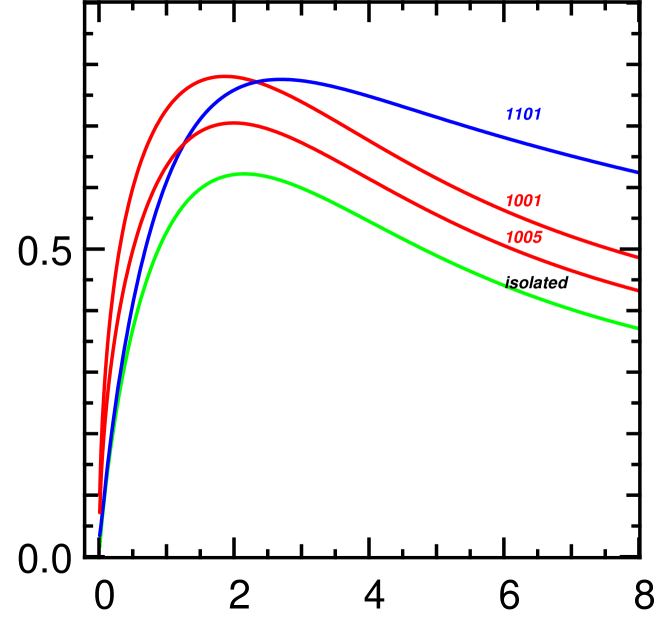
Figure 2: The rotation curves of some of the models in Table 2. The lower curve is that of an isolated exponential disk.

We can evaluate the strength of the instability visually and quantitatively. The endpoints of simulations 1005 and 1001 are shown in Figure 3, and a bar is clearly visible in the former. As an objective measure we use a logarithmic spiral decomposition of the surface density (Anathassoula & Sellwood 1986). We define the quantity

$$A_{p}={\sqrt{N}\over M_{\rm d}}\;\sum\limits_{j=1}^{N}m_{j}\exp[i(2\theta_{j}+p\ln R_{j})],$$ (20)

where $p$ is the logarithmic spiral wavenumber, $m_{j}$ is the mass, and $(R_{j},\theta_{j})$ are the cylindrical co-ordinates of a particle labelled by an index $j$. The factor outside the summation scales $A_{p}$ so that the expected value is unity if there is no significant structure at a given $p$. The factor of 2 in the argument of the exponential means that we pick out density perturbations with $m=2$ symmetry. For $p>0$ we have a trailing spiral and for $p<0$ a leading spiral. A bar has $p=0$. We measure $A_{p}$ approximately 40 times during each simulation, and consider the quantity $\left|A_{0}\right|$ defined as the average over the range $p\in[-1,1]$. In Figure 4 we show $\left|A_{0}\right|$ as a function of time for all the simulations. Those with visually identifiable bars (1005, 1105) show up clearly as having a significantly larger value of $\left|A_{0}\right|$. Thus both methods agree. We give an indication of whether a bar was present or not in Table 2.

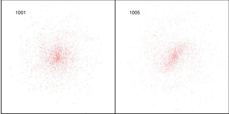
Figure 3: The endpoints of two of the simulations (showing only 4096 particles to avoid crowding). Simulation 1005 clearly shows a strong bar, while 1001 does not. The rotation curves of these two models are shown in Figure 2. The figures are bounded by the simulation box which is 8$R_{\rm d}$ on a side.

$\left|A_{0}\right|$

$t/T_{\rm d}$

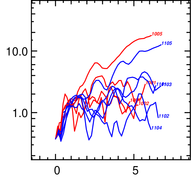
Figure 4: The strength of the bar $\left|A_{0}\right|$ as a function of time for the simulations in Table 2. Simulations 1005 and 1105 show clearly the presence of a bar, as shown in Figure 3. The time unit is $T_{\rm d}=2\pi(R_{\rm d}^{3}/GM_{\rm d})^{1/2}$.

It follows that the boundary $\epsilon_{\rm c}$ between global stability and a bar-forming instability lies between $\epsilon_{\rm m}=0.70$ and $\epsilon_{\rm m}=0.75$. The 10% quantile in Figure 1 combined with these values of $\epsilon_{\rm c}$ gives an upper limit to the mass-to-light ratio $\Upsilon_{I}<(1.85\pm.1)h$. The formal error only reflects the uncertainty in the value of $\epsilon_{\rm c}$. The upper limit would be higher if one had more tolerance for disks with apparent $\epsilon_{\rm m}<\epsilon_{\rm c}$. Nevertheless the limit is in agreement with independent direct measurements (see Section 6).

The critical value $\epsilon_{\rm c}$ is much lower than that obtained by ELN for their ‘FE’ models ($\epsilon_{\rm c}\approx 1.1$). ELN also conducted simulations with isothermal halos similar to ours, but they did not cover as much parameter space as their FE models, and were not analyzed in much detail. The obvious differences between our simulations and those of ELN are that our simulations are 3-dimensional, and that they have slightly better formal resolution. Resolution would not seem to explain our different conclusion. Indeed, we carried out simulations with $N=1024$ and a significantly larger softening length and reached the same conclusion. The difference could arise from the finite thickness of our disks. They have a vertical scale height of $0.2R_{\rm d}$, implying a formal eccentricity of $e=\sqrt{1-.2^{2}}=0.97$. Isolated stellar Maclaurin spheroids are already unstable at $e=0.97$. The added external potential may be enough to stabilize our disks but not those of ELN with $e=1$. A further difference between our simulations and those of ELN is the value of Toomre’s $Q$ and its dependence on radius. Most of the simulations of ELN use $Q(R)=\hbox{constant}=1.05$, whereas we use a profile with a broad minimum of $Q=1.2$ at $R\approx 2.4R_{\rm d}$. ELN also ran a few simulations with $Q$ a decreasing function of radius, and reported that their results were unchanged. The lower value of $Q$ would make their disks more prone to bar formation. Note however that typical values for galactic disks are even higher than in our simulations (Lewis & Freeman 1989, Bottema 1987, von Linden & Fuchs 1997).

Our results support the conclusion of ELN that $\epsilon_{\rm m}$ is a good indication of stability, independent of halo type and concentration (the Hernquist halos are more concentrated than the isothermal ones). One implication is that a modified Ostriker & Peebles criterion such as that considered by Christodoulou, Schlosman & Tohline (1995) is unlikely to be universal.

6 Independent determinations of $\Upsilon$

Limits on the mass-to-light ratio of the Galactic disk in the solar neighbourhood can be derived from a combination of kinematic measurements and star counts. Kuijken & Gilmore (1989) derive a local surface mass density in the disk of $40{M_{\sun}}/{\hbox{pc}}^{2}$, and star counts give a $V$-band luminosity density of $15{L_{\sun}}/{\hbox{pc}}^{2}$ (Gould, Bahcall & Flynn 1996). Dividing mass by light we obtain $\Upsilon_{V}=2.67$, and thus $\Upsilon_{I}\approx 1.9$ (assuming $V-I=1.0$). This number is independent of $h$, and hence is rather high compared with the upper limit derived from the $N$-body simulations. The data quoted by Bottema (1993) give a value of $\epsilon_{l}=1.37$ for the Galaxy, so for $\Upsilon_{I}\approx 1.9$ we obtain $\epsilon_{\rm m}\approx 1.0$. Thus despite having high $\Upsilon_{I}$ we conclude that the disk of the Galaxy should be globally stable.

Mass-to-light ratios can also be derived from pure stellar population synthesis arguments, although there is always some uncertainty arising from the poorly known initial mass function (IMF), particularly from the low-mass cut-off in the IMF. A few stellar population models are available (e.g., Bertelli et al 1994; Bruzual & Charlot 1993; Worthey 1994). For a Salpeter IMF, the mass-to-light ratio derived by various authors appear to agree within an accuracy of 25% (Charlot, Worthey & Bressan 1996). The predicted $\Upsilon_{I}$ depends on the metallicity and age of the stellar population. For a stellar population with age between 5-12 Gyr and with a solar metallicity, $\Upsilon_{I}$ is between $0.9$-$1.8$ for a constant star formation rate (cf Table 3 in de Jong 1996). For an exponential star formation law, the mass-to-light ratio is about 20% higher. The predicted values are in good agreement with the values derived from the instability analysis presented in this paper. In the comparison, we have neglected the uncertainty due to dust, since the Tully-Fisher studies already attempt to correct for its effect. Furthermore de Jong (1996) argues that dust reddening probably plays a minor role in the color gradients in disk galaxies. Nevertheless, the dust correction remains a nuisance in these comparisons.

$\Upsilon_{I}/h$

$\mu_{0}(I-\hbox{mag/sec}^{2})$

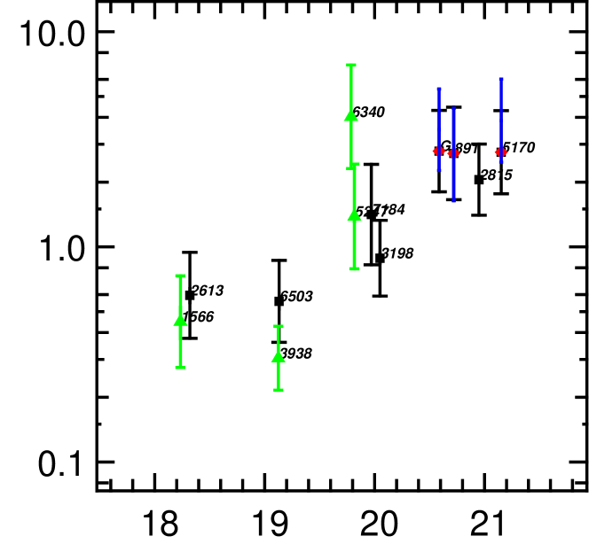
Figure 5: The mass-to-light ratio versus I-band central surface brightness for 12 galaxies from Bottema (1993) calculated according to equation (22). Each point is marked by its NGC number (or G for the Galaxy). For the Galaxy $\Upsilon_{I}$ has not been divided by $h$. Squares are for inclined galaxies; triangles for face-on galaxies; circles are additional points for highly inclined galaxies where $z_{0}$ is measured (otherwise $z_{0}/R_{\rm d}=0.2$ is assumed). The errorbars are estimated from the errors in the velocity dispersions.

A direct measurement of the mass-to-light ratio of extragalactic disks requires detailed kinematic studies such as that described by Bottema (1993). Bottema (1997) derives a value of $\Upsilon_{I}=(1.7\pm 0.5)h$ after somewhat uncertain processing of his data. The measurement of $\Upsilon$ relies on the relation between vertical velocity dispersion $\sigma_{z}$, surface density $\Sigma$ and vertical scale height $z_{0}$. Essentially, the larger the value of $\Sigma$, the hotter a disk has to be at constant $z_{0}$. For a disk which is well approximated by an isothermal sheet (cf. equation 18)

$$\sigma_{z}^{2}=\pi G\Sigma z_{0}$$ (21)

(e.g. Binney & Tremaine 1987). Assuming an exponential radial profile we can write the mass-to-light ratio as

$$\Upsilon={2G\sigma_{z}^{2}R_{\rm d}\over L_{\rm d}}{R_{\rm d}\over z_{0}}.$$ (22)

Taking account of the possible variations in vertical density profile in the disk, equation (22) represents an upper limit on $\Upsilon$ (Wielen & Fuchs 1983). Bottema measures $\sigma_{z}(R\!=\!0)$ for face-on galaxies, and asserts that $\sigma_{R}(R\!=\!R_{\rm d})=\sigma_{z}(R\!=\!0)$ for inclined galaxies (this is true for the Galaxy). Only 4 of the 12 galaxies are edge-on enough to measure $z_{0}$, so an assumption also has to be made about its value in the other galaxies. Bottema discusses this problem in some depth. Where it can be measured directly $z_{0}/R_{\rm d}\approx 0.2$ and does not vary by more than about 20 percent (Barteldrees & Dettmar 1994).

Figure 5 shows $\Upsilon_{I}$ calculated from equation (22) (assuming $z_{0}/R_{\rm d}=0.2$ where no measurement is available) plotted against $\mu_{0}$. The quantity plotted is independent of $h$. In the case of the Galaxy $\Upsilon_{I}$ has not been divided by $h$. The first impression of this figure is a marked trend of smaller $\Upsilon_{I}$ for higher surface brightness galaxies (low $\mu_{0}$ in magnitudes). The range of values of $\Upsilon_{I}$ is also large (about a factor of $10$ between smallest and largest values). This is in marked conflict with the received wisdom regarding mass-to-light ratios of galactic disks, based on the uniformity of the colours of stellar populations (de Jong 1996). Indeed taken at face value, the trend in Figure 5 is so strong that when applied to equation (17) it should produce an anti-correlation between $\epsilon_{l}$ and $\mu_{0}$ for constant $m_{d}$.

$\epsilon_{\rm m}$

$\mu_{0}(I-\hbox{mag/sec}^{2})$

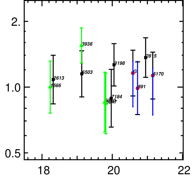
Figure 6: Shows $\epsilon_{\rm m}$ for the galaxies of Bottema (1993) given the values of $\Upsilon_{I}$ from Figure 5.

How should we interpret Figure 5? We would like to see many more data before any strong conclusions are drawn. One can separate the galaxies by eye into two groups: one with high surface brightness ($\mu_{0}<19.5$) and low $\Upsilon_{I}$, and the other with lower surface brightness ($\mu_{0}>19.5$) and higher $\Upsilon_{I}$. Of the four galaxies with $\mu_{0}<19.5$, two have significant non-stellar contributions to their luminosity (3938 and 1566) which could bias them artificially towards the bottom left of Figure 5. Notice that few galaxies in the MF sample have surface brightness as high as these four galaxies. Taken on their own, the galaxies with $\mu_{0}>19.5$ have values of $\Upsilon_{I}$ which are perhaps not a strong function of $\mu_{0}$.

From equations (5) & (22) we can obtain a simple expression for $\epsilon_{\rm m}$ in terms of kinematical quantities:

$$\epsilon_{\rm m}={v_{\rm m}\over\sigma_{z}}\sqrt{z_{0}\over 2R_{\rm d}}.$$ (23)

Figure 6 shows the values of $\epsilon_{\rm m}$ for the galaxies in Figure 5 calculated from equation (23). They are all $\ga 0.75$ so the values of $\Upsilon_{I}$ in Figure 5 are consistent with the disks being globally stable.

There remains a constraint on the average $\Upsilon_{I}$ as a function of $\mu_{0}$ from the theory of disk formation. As was mentioned in Section 4, the observed positive correlation in Figure 1 is consistent with $A$ being at most a weak function of $\mu_{0}$, particularly for the high surface brightness galaxies. This conclusion is expected to be only weakly dependent on the detailed model of disk formation—only the normalisation depends somewhat on the cosmological model (Mo, Mao & White 1997). The mass-to-light ratio $\Upsilon_{I}$ required to match the Tully-Fisher relation is in the range of 1 to $2h$, consistent with those obtained from the stability analysis presented here and models of stellar population synthesis. Whether it is actually consistent with Figure 5 is unclear until we have more data. If such a trend exists, the small scatter in the Tully-Fisher amplitude $A$ would require a nearly linear correlation between $m_{d}$ and $\Upsilon_{I}$ (cf equation 14).

7 Discussion

Global instability in a disk leads to bar formation, so it is natural to assume that barred galaxies form in this way (e.g. Sellwood 1996). If the correlation of $\epsilon_{l}$ with $\mu_{0}$ really reflects a correlation of $\epsilon_{\rm m}$ with $\mu_{0}$, then we should expect galaxies with smaller values of $\epsilon_{l}$ to form bars. No such effect is visible in the MF data. The distribution of barred types is indistinguishable from that of disk galaxies as a whole (Figure 1). Bar formation does not have to be spontaneous: it could be induced by a perturbation from a close encounter with another galaxy (Noguchi 1996), or from an interaction between the disk and the halo. Perhaps all disks have $\Upsilon_{I}$ such that a bar does not form spontaneously, but they are equally susceptible to induced bar formation. This is consistent with the values of $\epsilon_{\rm m}$ in Figure 6. Note however that the barred fraction in the MF data is low ($\approx 10\%$) compared to that reported by other authors (e.g. Sellwood & Wilkinson 1993 give a fraction of around 30%). Further discussion of this important question is outside the scope of the present work.

Clearly it is important to extend the range of data analysed in Section 6. This requires a good HI rotation curve for each galaxy, and high quality spectroscopy at least along the major axis of the galaxy. Ideally one would choose the brightest members of a large pre-defined sample (such as that of Mathewson & Ford 1996) and follow them up with a high spatial resolution spectrograph. Kinematic information in more than one dimension is also advantageous since it removes some of the uncertainties in the deprojection of the velocity ellipsoid. A number of two dimensional spectrographs are due to come on line shortly, and these may be well suited to the problem. The biggest uncertainty in the determination of $\Upsilon_{I}$ will remain that associated with the value of $z_{0}$. Efforts should therefore be made to analyse as many edge on galaxies as possible to try to improve on existing determinations of the distribution of $z_{0}/R_{\rm d}$ (e.g. Barteldrees & Dettmar 1994).

Appendix

Here we describe how values of $R_{\rm d}$, $\mu_{0}$ and $L$ were derived from the published quantities of Mathewson & Ford (1996). The published data list total magnitudes, and face-on corrected isophotal quantities: average surface brightness and isophotal diameter at $\mu=23.5\hbox{mag/sec}^{2}$. Assuming an exponential disk we have a surface brightness profile

$$\mu(R)=\mu_{0}\exp(-\alpha),~{}~{}\alpha\equiv{R\over R_{d}},$$ (24)

and for a bulge to disk ratio $f$ we have (outside the bulge)

$$L(R)=L_{\rm d}\left(1+f-\exp(-\alpha)(\alpha+1)\right).$$ (25)

From equation (25) the average surface brightness inside radius $R$ is

$$\bar{\mu}={L(R)\over\pi R^{2}}={2\mu_{0}\over\alpha^{2}}\left(1+f-\exp(-\alpha)(\alpha+1)\right),$$ (26)

where we have used $L_{\rm d}=2\pi\mu_{0}R_{\rm d}^{2}$. Combining equations (25) and (26) we obtain

$${\bar{\mu}\over\mu}={\exp(\alpha)(1+f)-(\alpha+1)\over\alpha^{2}}.$$ (27)

Given $f$ and $\bar{\mu}/\mu$ we can solve equation (27) numerically to find $\alpha$. Then we have $R_{\rm d}=R/\alpha$, and $\mu_{0}=\mu\exp(\alpha)$.

In Table 1 the data labelled MF is obtained by setting $f=0$ (no bulge). Those labelled MFD have a crude bulge subtraction applied as follows. If the galaxy is classified Sbc or Sc a value of $f$ is initially chosen randomly from a uniform distrubution in the range $[0,.2]$. If it is Sa or Sb $f$ is similarly chosen in the range $[0,.4]$. This covers about 80% of the galaxies, and for the remainder we simply set $f=0$. For too large a value of $f$, equation (27) does not have a solution for positive real $\alpha$. If $f$ is initially too large, it is reduced by a factor of $3/4$. This factor is applied repeatedly until a solution is found.

References

- [1] Anathassoula, E. & Sellwood, J.A., 1986, MNRAS, 221, 195
- [2]
- [3] Bertelli G., Bressan A., Chiosi C., Fagotto F., & Nasi E. 1994, A&AS, 106, 275
- [4] Barteldrees, A. & Dettmar, R-J., 1994, AA Supp., 103, 475
- [5]
- [6] Binney, J., and Tremaine, S. 1987, Galactic Dynamics, Princeton: Princeton University Press.
- [7] Bottema, R., 1987, A&A, 178, 77
- [8]
- [9] Bottema, R., 1993, A&A, 275, 16
- [10]
- [11] Bottema, R., 1997, preprint (astro-ph/9706230)
- [12] Bruzual G.A., Charlot S. 1993, ApJ, 405, 538
- [13] Burstein, D., Bender, R., Faber, S.M. & Nolthenius, R., 1997, preprint (astro-ph/9707037)
- [14] Carignan, C. & Freeman, K.C., 1985, ApJ, 294, 494
- [15]
- [16] Chandrasekhar, S., 1969, Ellipsoidal Figures of Equilibrium, Newhaven: Yale University Press.
- [17] Charlot S., Worthey S. & Bressan A. 1996, ApJ, 457, 625
- [18] Christodoulou, D.M., Schlosman, I. & Tohline J.E., 1995, ApJ, 443, 551
- [19]
- [20] Couchman, H.M.P., Pearce, F.R., & Thomas, P.A., 1995, ApJ, 452, 797
- [21]
- [22] Courteau S., 1996, ApJS, 103, 363
- [23]
- [24] Courteau S., 1997, ApJS, 000, in press
- [25]
- [26] Courteau S. & Rix H.-W. 1997, preprint (astro-ph/9707290)
- [27] Dalcanton, J.J, Spergel, D.N. & Summers, F.J., 1997, ApJ, 482, 659
- [28]
- [29] Dale, D.A., Giovanelli, R., Haynes, M.P. & Scodeggio, M., 1997, AJ, 114, 455
- [30]
- [31] de Blok, W.J.G. & McGaugh, S.S., 1997, preprint (astro-ph/9704274).
- [32] de Jong, R.S., 1996, A&A, 313, 377
- [33]
- [34] Efstathiou, G., Lake, G., & Negroponte, J., 1982, MNRAS, 199, 1069 (ELN)
- [35]
- [36] Fall, S.M. & Estafthiou, G., 1980, MNRAS, 193, 189
- [37]
- [38] Freeman, K.C., 1970, ApJ, 160, 811
- [39]
- [40] Gould, A., Bahcall, J.N. & Flynn, C., 1996, ApJ, 465, 759
- [41]
- [42] Giovanelli, R., Haynes, M.P., da Costa, L.N., Freudling, W., Salzer, J.J. & Wegner, G., 1997, preprint (astro-ph/9612072)
- [43] Hernquist, L., 1990, ApJ, 356, 359
- [44]
- [45] Hernquist, L., 1993, ApJS, 86, 389
- [46]
- [47] Kravtsov, A.V., Klypin, A.A., Bullock, J.S. & Primack, J.R., preprint astro-ph/9708176.
- [48] Kuijken, K. & Gilmore, G., 1989, MNRAS, 239, 650
- [49]
- [50] Lewis, J. & Freeman, K., 1989, AJ, 299, 633
- [51]
- [52] Mathewson, D.S. & Ford, L. 1996, ApJS, 107, 97
- [53]
- [54] McGaugh S.S. & de Blok W.J.G., 1997, ApJ, 481, 689
- [55] Miller, R.H., 1978, ApJ, 223, 811
- [56]
- [57] Miller R.H., Smith B.F., 1978, ApJ, 227, 407
- [58]
- [59] Mo, H.J., Mao, S. & White S.D.M. 1997, MNRAS, in press (astro-ph/9707093)
- [60] Moore B., Governato F., Quinn T., Stadel J., Lake G. 1997, preprint (astro-ph/9709051)
- [61] Navarro, J.F., Frenk, C.S., & White, S.D.M., 1996, ApJ, 462, 563
- [62]
- [63] Noguchi, M. 1996, in Barred Galaxies, IAU Colloquium 157, San Fransisco: ASP, p. 339.
- [64] Ostriker, J.P. & Peebles, P.J.E., 1973, ApJ, 186, 467
- [65]
- [66] Persic, M. & Salucci, P., 1991, ApJ, 285, 307
- [67]
- [68] Raychaudhury, S., von Braun, K., Bernstein, G.M. & Guhathakurta, P., 1997, AJ, 113, 2046
- [69]
- [70] Sellwood, J.A., 1996, p. 256 in Barred Galaxies, IAU Colloquium 157, San Fransisco: ASP, p. 259.
- [71] Sellwood, J.A., & Wilkinson, A., 1993, Rep. Prog. Phys., 56, 173
- [72]
- [73] Shanks, T., 1997, preprint (astro-ph/9702148)
- [74] Toomre, A., 1963, ApJ, 138, 385
- [75]
- [76] Tully, R.B. & Fisher, J.R., 1977, A&A, 54, 661
- [77]
- [78] van der Kruit, P.C. & Searle., L., 1981, A&A, 95, 105
- [79]
- [80] von Linden, S. & Fuchs, B., 1997, MNRAS, in press, (astro-ph/9708028)
- [81]
- [82] Wielen, R. & Fuchs, B., 1983, in Kinematics, Dynamics and Structure of the Milky Way, ed W.L.H. Shuter (Dordecht: Reidel), p. 81.
- [83] Worthey G. 1994, ApJS, 95, 107