Cosmic Microwave Background Anisotropies from Scaling Seeds: Generic Properties of the Correlation Functions

Abstract

In this work we present a partially new method to analyze fluctuations which are induced by causal scaling seeds. We show that the power spectra due to this kind of seed perturbations are determined by five analytic functions, which we determine numerically for a special example. We put forward the view that, even if recent work disfavors the models with cosmic strings and global $O(4)$ texture, causal scaling seed perturbations merit a more thorough and general analysis, which we initiate in this paper.

I Introduction

At present, two ideas to explain the origin of large scale structure in the universe are primarily investigated:

• Perturbations in the energy density of matter may have emerged from quantum fluctuations, which, during a phase of inflationary expansion, are stretched beyond the Hubble scale and ’freeze in’ as classical fluctuations in the energy density of the cosmic fluid[1]. These small initial fluctuations then evolve according to linear cosmological perturbation theory.

• A phase transition in the early universe may lead to topological defects which seed fluctuations in the cosmic fluid [2]. In this case, the fluid fluctuations vanish initially and evolve according to inhomogeneous cosmic perturbation equations. The stress energy of the topological defects plays the role of the source term. In order for the gravitational field of the defects to be sufficiently strong to seed cosmic structure, we have to require $\epsilon=4\pi G\eta^{2}\sim 10^{-5}$, where $\eta$ denotes the energy scale of the phase transition. This yields $\eta\sim 10^{16}$GeV, a typical GUT scale. Topological defects which neither over-close the universe nor die out are either cosmic strings or global defects.

The anisotropies in the cosmic microwave background (CMB) provide an important tool to discriminate between different models. On very large angular scales both classes of models lead to a Harrison Zel’dovich spectrum of fluctuations. For inflationary models this can easily be derived analytically. For defect models, the spectra were originally found numerically [3, 4, 5]. Analytical arguments for this behavior are given in [6]. On intermediate scales, inflationary models predict a series of peaks due to acoustic oscillations in the baryon/photon fluid prior to recombination[7]. Present observations seem to confirm these peaks even though the error bars are still considerable[8].

Recently, several investigations led to the conclusion that cosmic strings [9, 10] and global ${\cal O}(N)$ defects [11, 12, 13] do not reproduce the acoustic peaks indicated by present data. This led [12] and [10] to the conclusion that models of cosmic structure formation with scaling causal defects are ruled out.

However, in a very simple parameterization of two families of more general scaling causal seed models, we were able to fit present data very well[13]. We are thus convinced that it is too early yet to completely abandon scaling causal seeds as a mechanism for structure formation. In contrary, we think it is extremely useful to study them in full generality, ignoring in a first step the physical origin of the seeds. This purely phenomenological point of view is analogous to inflationary models where one sometimes manufactures the inflationary potential to yield the required spectrum of initial perturbations.

To determine the power spectrum of the radiation and matter perturbations induced by seeds, we need to know the two point correlation functions of the seed energy momentum tensor. In this paper we present a simple parameterization of these functions and point out an error frequently made in the literature. We then exemplify our findings with the large $N$ limit of global scalar fields [14, 15].

For simplicity, we work in a spatially flat Friedman universe. The metric is thus given by

$\displaystyle ds^{2}=a(t)^{2}(dt^{2}-\delta_{ij}dx^{i}dx^{j})~{},$

where $t$ denotes conformal time.

II Correlation functions of causal scaling seeds

We define seeds to be any non-uniformly distributed form of energy, which contributes only a small fraction to the total energy density of the universe and which interacts with the cosmic fluid only gravitationally.

We parameterize the energy momentum tensor of the seed by

$$T^{(seed)}_{\mu\nu}=M^{2}\Theta_{\mu\nu}~{},$$ (1)

where $M$ denotes a typical energy of the seed and $\Theta_{\mu\nu}$ is a random variable. We assume that ensemble averages and and spatial averaging coincide, the usual ergodicity hypothesis. Furthermore, we assume the random process $\Theta_{\mu\nu}$ to be spatially homogeneous and isotropic, so that the two point correlation function

$$\langle\Theta_{\mu\nu}({\bf x},t)\Theta_{\lambda\rho}({\bf x+y},t^{\prime})\rangle=$$ (3)

$${1\over V}\int\Theta_{\mu\nu}({\bf x},t)\Theta_{\lambda\rho}({\bf x+y},t^{\prime})d^{3}x\equiv C_{\mu\nu\lambda\rho}({\bf y},t,t^{\prime})$$

is a function of the difference $\bf y$ only. Due to the expansion of the universe, which breaks time translation symmetry, we however expect $C$ to depend on $t$ and $t^{\prime}$ and not just on the difference $t-t^{\prime}$. We consider causal seeds. Causality requires

$$C_{\nu\mu\lambda\rho}({\bf y},t)=0,\mbox{ if }~{}~{}|{\bf y}|>t+t^{\prime}~{}.$$ (4)

The two point function in position space thus has compact support which implies that its Fourier transform is analytic.

We define a seed to be scaling, if the Fourier transform,

$$\widehat{C}_{\mu\nu\lambda\rho}({\bf k},t,t^{\prime})=\langle\widehat{\Theta}_{\mu\nu}({\bf k},t)\widehat{\Theta}^{*}_{\lambda\rho}({\bf k},t^{\prime})\rangle~{},$$ (5)

contains no dimensional parameter other than $t,t^{\prime}$ and $k$. This implies that the Ricci curvature induced by the seeds is a function of $k$ and $t$ only, multiplied by the dimensionless parameter $\epsilon=4\pi GM^{2}$. Since we define Fourier transforms with the normalization

$$\hat{f}({\bf k}) = {1\over\sqrt{V}}\int d^{3}xf({\bf x})\exp(i{\bf kx})~{};$$ (6)

$$f({\bf x}) = {\sqrt{V}\over(2\pi)^{3}}\int d^{3}k\hat{f}({\bf k})\exp(-i{\bf kx})~{},$$ (7)

and since $\Theta_{\mu\nu}({\bf x},t)$ has the dimension of (length)^-2, $\widehat{C}$ has the dimension of an inverse length. From scaling we therefore conclude that for purely dimensional reasons, we can write the correlations functions in the form

$$\hat{C}_{\mu\nu\lambda\rho}({\bf k},t,t^{\prime})={1\over\sqrt{tt^{\prime}}}F_{\mu\nu\lambda\rho}(\sqrt{tt^{\prime}}\cdot{\bf k},t^{\prime}/t)~{},$$ (8)

where $F_{\mu\nu\lambda\rho}$ is a dimensionless function of the four variables $z_{i}\equiv\sqrt{t^{\prime}t}k_{i}$ and $r\equiv t^{\prime}/t$, which is analytic in $z_{i}$.

We also require the seed to decay inside the horizon, which implies

$$\hat{C}_{\mu\nu\lambda\rho}({\bf k},t,t^{\prime})\rightarrow_{kt\rightarrow\infty}=\hat{C}_{\mu\nu\lambda\rho}({\bf k},t,t^{\prime})\rightarrow_{kt^{\prime}\rightarrow\infty}=0~{}.$$ (9)

Furthermore, since the seeds interact with the cosmic fluid only gravitationally, $\Theta$ satisfies covariant energy momentum conservation,

$$\Theta^{\mu\nu};_{\nu}=0~{}.$$ (10)

With the help of these four equations, we can, for example, express the temporal components, $\Theta_{0\mu}$ in terms of the spatial ones, $\Theta_{ij}$. The seed correlations are thus fully determined by the spatial correlation functions $\widehat{C}_{ijlm}$. Statistical isotropy, scaling and symmetry in $i,j$ and $l,m$ as well as under the transformation $i,j;k;t\rightarrow l,m;-k;t^{\prime}$ require the following form for the spatial correlation functions:

$$\widehat{C}_{ijlm}({\bf k},t,t^{\prime})=$$ (15)

$${1\over\sqrt{tt^{\prime}}}[z_{i}z_{j}z_{l}z_{m}F_{1}(z^{2},r)+$$

$$(z_{i}z_{l}\delta_{jm}+z_{i}z_{m}\delta_{jl}+z_{j}z_{l}\delta_{im}+z_{j}z_{m}\delta_{il})F_{2}(z^{2},r)+$$

$$z_{i}z_{j}\delta_{lm}F_{3}(z^{2},r)/r+z_{l}z_{m}\delta_{ij}F_{3}(z^{2},1/r)r+$$

$$+\delta_{ij}\delta_{lm}F_{4}(z^{2},r)+(\delta_{il}\delta_{jm}+\delta_{im}\delta_{jl})F_{5}(z^{2},r)]~{},$$

where the functions $F_{a}$ are analytical functions of $z^{2}\equiv tt^{\prime}k^{2}$, and for $a\neq 3$ they are invariant under the transformation $r\rightarrow 1/r$, $F_{a}(z^{2},r)=F_{a}(z^{2},1/r)$. The positivity of the power spectra $\hat{C}_{ijij}({\bf k},t,t)=\langle|\Theta_{ij}|^{2}\rangle$ leads to a series of positivity conditions for the functions $F_{a}$:

$$0 \leq F_{5}(z^{2},1)~{},$$ (16)

$$0 \leq F_{4}(z^{2},1)+2F_{5}(z^{2},1)~{},$$ (17)

$$0 \leq z^{2}F_{2}(z^{2},1)+F_{5}(z^{2},1)~{},$$ (18)

$$0 \leq z^{4}F_{1}(z^{2},1)+4z^{2}F_{2}(z^{2},1)+3F_{5}(z^{2},1)~{},$$ (19)

$$0 \leq z^{4}F_{1}(z^{2},1)+2z^{2}(F_{3}(z^{2},1)+2F_{2}(z^{2},1))$$ (21)

$$+F_{4}(z^{2},1)+2F_{5}(z^{2},1)~{}.$$

Since $\hat{C}_{ijlm}$ is the Fourier transform of a real function,

$$\hat{C}_{ijlm}({\bf k},t,t^{\prime})^{*}=\hat{C}_{ijlm}(-{\bf k},t,t^{\prime})~{},$$ (22)

and thus the ansatz (15) implies that the functions $F_{a}(z^{2},r)$ are real. Furthermore, decay inside the horizon (condition (9)) yields

$$\lim_{z^{2}r\rightarrow\infty}F_{a}(z^{2},r)=\lim_{z^{2}/r\rightarrow\infty}F_{a}(z^{2},r)=0~{}.$$ (23)

In addition, analyticity implies that the functions $F_{a}$ do not diverge in the limit $z\rightarrow 0$, thus

$\displaystyle\lim_{z\rightarrow 0}F_{a}(z,r)=A_{a}(r)$

with

$\displaystyle A_{a}(r)=A_{a}(1/r)~{}\mbox{ for all }a\neq 3~{}.$

As an example, we have worked out the functions $F_{1}$ to $F_{5}$ in the large $N$ limit of global scalar field seeds. A discussion of this simple model of scaling causal seeds ands its relation to the texture model of structure formation can be found in [14] and [15] . In Figs. 1 and 2 we present the functions $F_{5}(z^{2},r)$ and $F_{2}(z^{2},r)$.

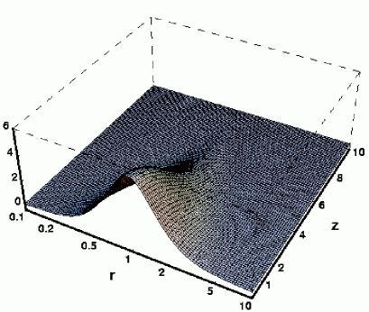
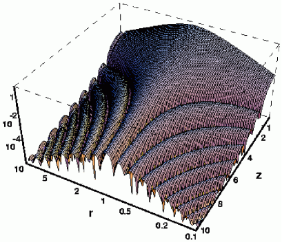
FIG. 1.: The function $F_{5}(z,r)$, linear (top) and $|F_{5}(z,r)|$ logarithmic are shown. Because of their small amplitude, the oscillations are virtually invisible in the linear plot. To show the symmetry $r\rightarrow 1/r$, the $r$-axis is chosen logarithmic in both plots.

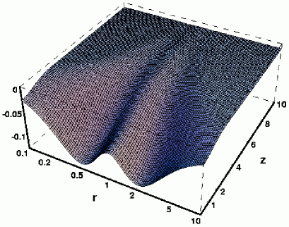
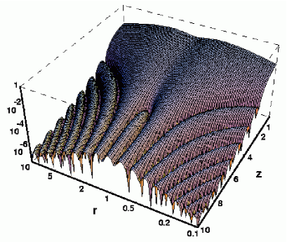
FIG. 2.: The same as Fig. 1 for the function $F_{2}(z,r)$.

The symmetry under the transition $r\rightarrow 1/r$ is clearly visible. Also the conditions that $F_{a}\rightarrow 0$ if either $z\rightarrow\infty$ or $r\rightarrow 0$ or $r\rightarrow\infty$ which follows from Eq. (23) is evidently satisfied. For fixed $z$ the functions oscillate with a frequency which grows with $z$. Since the amplitude decays rapidly, these oscillations are only visible in the log-plots. The correlations always decay like power laws, never exponentially.

The equal time correlation functions, $F_{1}(z^{2},1)$ to $F_{5}(z^{2},1)$ are plotted in Fig. 3. In Fig. 4 we show $A_{a}(r)$.

FIG. 3.: The functions $|F_{i}(z,1)|$ are shown. The zeros are visible as spikes in the log-plot. (Further below, at $z\sim 30$, also $F_{1}$ passes through zero.)

FIG. 4.: The functions $|A_{i}(r)|=|F_{i}(0,r)|$ are shown. As discussed in the text, all of them except $A_{3}$ are symmetrical under the transition $r\rightarrow 1/r$.

All the functions, except $F_{5}$ which is constrained by Eq. (16) go through $0$ (For $F_{1}$ the passage through $0$ is not visible since it occurs only at $z\simeq 30$). We have also verified the positivity constraints Eq. (17) to Eq. (21). The asymptotic behavior of the functions can be obtained analytically. The same is true for the functions $A_{1}$ to $A_{5}$. As argued above, all the functions $A_{i}$ except $A_{3}$ are symmetric under $r\rightarrow 1/r$. The techniques employed to calculate the functions $F_{i}$ are analogous to those explained in [15].

III Scalar, vector and tensor decomposition and CMB anisotropies

The energy momentum tensor of seeds is often split into scalar, vector and tensor perturbations, since the time evolution of each of these components is independent. Furthermore, due to statistical isotropy, the scalar, vector and tensor modes are uncorrelated.

A suitable parameterization of this decomposition is

$$\Theta_{ij}=\delta_{ij}f_{p}-(k_{i}k_{j}-{k^{2}\over 3}\delta_{ij})f_{\pi}+{1\over 2}(w_{i}k_{j}+w_{j}k_{i})+\tau_{ij}~{},$$ (24)

where $f_{p},~{}f_{\pi}$ are arbitrary random functions of k; w is a transverse vector, ${\bf w\cdot k}=0$; and $\tau_{ij}$ is a symmetric, traceless, transverse tensor, $\tau^{i}_{i}=\tau_{ij}k^{j}=0$. The variables $f{\bf.}~{},{\bf w}$ and $\tau_{ij}$ represent the scalar, vector and tensor degrees of freedom of $\Theta_{ij}$. The functions $F_{1}$ to $F_{5}$ determine the correlations: To work out the correlation functions we use

$$f_{p} = {1\over 3}\Theta_{i}^{i}={1\over 3}\delta_{ij}\Theta^{ij}~{},$$ (25)

$$f_{\pi} = -{3\over 2k^{2}}(\hat{k}^{i}\hat{k}^{j}-{1\over 3}\delta_{ij})\Theta_{ij}={3\over 2k^{2}}S_{ij}\Theta^{ij}~{},$$ (26)

$$w_{i} = {2\over k}(\delta_{i}^{~{}l}\hat{k}^{m}-\hat{k}_{i}\hat{k}^{l}\hat{k}^{m})\Theta_{lm}=V_{i}^{~{}lm}\Theta_{lm}~{},$$ (27)

$$\tau_{ij} = (P_{il}P_{jm}-(1/2)P_{ij}P_{lm})P^{ma}P^{lb}\Theta_{ab}$$ (28)

$$= T_{ij}^{~{}~{}ab}\Theta_{ab}~{},$$ (29)

where $$P_{ij}=\delta_{ij}-\hat{k}_{i}\hat{k}_{j}~{}~{}~{},~{}~{}~{}\hat{k}^{i}=k^{i}/k$$ (30)

$P_{i}^{~{}j}$ is the projection operator onto the space orthogonal to k and $S_{ij}$, $V_{i}^{~{}lm}$ and $T_{ij}^{~{}~{}ab}$ are the projection operators to the scalar vector and tensor parts of $\Theta_{ij}$.

Using these identities and our ansatz (15), one easily verifies

$$\langle f_{p}(t)w_{i}^{*}(t^{\prime})\rangle = \langle f_{\pi}(t)w_{i}^{*}(t^{\prime})\rangle=0$$ (31)

$$\langle f_{p}(t)\tau_{ij}^{*}(t^{\prime})\rangle = \langle f_{p}i(t)\tau_{ij}^{*}(t^{\prime})\rangle=0$$ (32)

$$\langle w_{i}(t)\tau_{jl}(t^{\prime})\rangle = 0$$ (33)

$$\langle f_{p}(t)f_{p}^{*}(t^{\prime})\rangle = {1\over 3\sqrt{tt^{\prime}}}[2F_{5}(z^{2},r)+3F_{4}(z^{2},r)$$ (36)

$$+z^{2}(F_{3}(z^{2},r)/r+F_{3}(z^{2},1/r)r)+$$

$${4\over 3}z^{2}F_{2}(z^{2},r)+{1\over 3}z^{4}F_{1}(z^{2},r)]$$

$$\langle f_{\pi}(t)f_{\pi}^{*}(t^{\prime})\rangle = {1\over\sqrt{tt^{\prime}}k^{4}}[3F_{5}+4z^{2}F_{2}+z^{4}F_{1}]$$ (37)

$$\langle f_{p}(t)f_{\pi}^{*}(t^{\prime})\rangle=$$ (39)

$$-\sqrt{tt^{\prime}}[{1\over 3}z^{2}F_{1}(z^{2},r)+{4\over 3}F_{2}(z^{2},r)+rF_{3}(z^{2},1/r)]$$

$$\langle w_{i}(t)w_{j}^{*}(t^{\prime})\rangle=$$ (41)

$${4\over k^{4}\sqrt{tt^{\prime}}}[F_{5}+z^{2}F_{2}](k^{2}\delta_{ij}-k_{i}k_{j})$$

$$\langle\tau_{ij}(t)\tau^{*}_{lm}(t^{\prime})\rangle=$$ (45)

$${1\over\sqrt{tt^{\prime}}}F_{5}[\delta_{il}\delta_{jm}+\delta_{im}\delta_{jl}-\delta_{ij}\delta_{lm}+k^{-2}(\delta_{ij}k_{l}k_{m}+$$

$$\delta_{lm}k_{i}k_{j}-\delta_{il}k_{j}k_{m}-\delta_{im}k_{l}k_{j}-\delta_{jl}k_{i}k_{m}-\delta_{jm}k_{l}k_{i})+$$

$$k^{-4}k_{i}k_{j}k_{l}k_{m}]~{}.$$

It is interesting to note that although $\widehat{C}_{ijlm}$ is analytic, the correlation functions of the scalar vector and tensor components, in general, are not. The reason for that is that the projection operators $S,V$ and $T$ are not analytic. This is important. It implies, e.g., that the anisotropic stresses in general have a white noise and not a $k^{4}$ spectrum as erroneously concluded in [16, 17, 18]. The scalar anisotropic stress potential thus diverges on large scales, $\langle|f_{\pi}|^{2}\rangle\propto 1/(tk^{4})$ for $kt\ll 1$. A result which we also have obtained in the large-$N$ limit and in numerical simulations of $O(N)$ models. The power spectrum of the scalar anisotropic stress potential $f_{\pi}$ is analytic if and only if vector and tensor perturbations are absent, $F_{5}=F_{2}=0$. In the generic situation, $F_{5}(z=0,r=1)=A_{5}(1)\neq 0$. We thus expect the following relation between scalar vector and tensor perturbations of the gravitational field on super-horizon scales, $x\equiv kt\ll 1$: (The equations for the scalar, vector and tensor gravitational potentials in terms of $f.$, w and $\tau_{ij}$ can be found in [19] and [20].)

$$\langle|\Phi-\Psi|^{2}\rangle \sim {12\epsilon^{2}\over tk^{4}}A_{5}(1)$$ (46)

$$\langle|\sigma_{i}|^{2}\rangle \sim {16\epsilon^{2}t\over k^{2}}A_{5}(1)$$ (47)

$$\langle|h_{ij}|^{2}\rangle \sim 4\epsilon^{2}t^{3}A_{5}(1)~{},$$ (48)

where $\Psi$ and $\Phi$ are the Bardeen potentials, $\sigma$ is the vector contribution to the shear of the $t=$const. slices and $h_{ij}$ are tensor perturbations of the metric.

If it would be solely super horizon perturbations which induce the large scale CMB anisotropies, this could be translated into a ratio between the scalar, vector and tensor contributions to the $C_{\ell}$’s on large scales, $\ell\stackrel{{\scriptstyle<}}{{\sim}}50$. However, since the main contribution to the CMB anisotropies is induced at horizon crossing, $x=1$ (see below) the above relations cannot be translated directly and we can just learn that one expects, in general, contributions of the same order of magnitude from scalar, vector and tensor perturbations.

Finally, we want to discuss in some detail the CMB anisotropies induced from scalar perturbations. In this case, the gravitational perturbation equations (see e.g. [19, 20]) imply

$$\Phi+\Psi=-2\epsilon f_{\pi}~{}.$$ (49)

Especially, if $\Phi$ has a white noise spectrum due to ’compensation’ [21], this leads to a $k^{-4}$ spectrum for $\Psi$ and for the combination $\Phi-\Psi$ which enters in Eq. (51).

This finding is in contradiction with [16, 17], which predict a white noise spectrum for $\Psi$, but it is not in conflict with the Harrison Zel’dovich spectrum of CMB fluctuations which has been obtained numerically in [3, 4, 5]. This can be seen by the following simple argument: Since topological defects decay inside the horizon, the Bardeen potentials on sub-horizon scales are dominated by the contribution from dark matter and thus roughly constant. The integrated Sachs Wolfe term then contributes only up to horizon scales. Therefore, using the fact that for defect models $D_{g}$ and $V$ are much smaller than the Bardeen potentials on super-horizon scales (see [21]), we obtain

$$(\Delta T/T)_{\ell}(k)|_{SW}\sim(\Phi-\Psi)(k,x_{dec})j_{\ell}(x_{0}-x_{dec})$$ (51)

$$+\int_{x_{dec}}^{1}({\Phi}^{\prime}-{\Psi}^{\prime})(k,x)j_{\ell}(x_{0}-x)dx~{},$$

where $x=kt$ and prime stands for derivative w.r.t. $x$. The lower boundary of the integrated term roughly cancels the ordinary Sachs Wolfe contribution and the upper boundary leads, to

$$\langle|(\Delta T/T)_{\ell}(k)|^{2}\rangle|_{SW}\sim$$ (53)

$${\epsilon^{2}\over k^{3}}[3F_{5}(1)+4F_{2}(1)+F_{3}(1)]j_{\ell}^{2}(x_{0})~{},$$

a Harrison-Zel’dovich spectrum. The main ingredients for this result are the decay of the sources inside the horizon as well as scaling, the rest follows for purely dimensional reasons.

IV Conclusions

In this paper, we outline a procedure to investigate causal scaling seed perturbations. We show, that the large number of seed correlations, which determine fully the induced power spectra of dark matter and CMB photons, can be cast in only five analytic functions with certain well defined properties. We schematically estimate the large scale CMB anisotropies induced. However, we are convinced that the relative amplitudes of large scale CMB anisotropies and the acoustic peaks as well as the dark matter power spectrum depend on details of the model and thus scaling causal seeds cannot be ruled out from studies of specific models. This finding is also confirmed in[13].

Our work is just the beginning of a program to be carried out which goes in different directions and to which we invite researchers in the field to participate. Some of the questions which should be explored are the following:

• Are there further general restrictions for the correlation functions which have not been mentioned here?

• Given the functions $F_{1}$ to $F_{5}$ what is the exact expression for the $C_{\ell}$’s and the dark matter power spectrum? What are good approximations?

• Are there simple conditions which the functions $F_{1}$ to $F_{5}$ have to satisfy in order to lead to power spectra which are in agreement with data.

• Are there physically plausible causal scaling seed models other than topological defects?

Acknowledgment      This work is partially supported by the Swiss NSF. Numerical simulations have been performed at the Centro Svizzero di Calcolo Scientifico (CSCS). It is a pleasure to thank P. Ferreira, M. Sakellariadou and N. Deruelle for stimulating discussions.

REFERENCES

- [1] J.M. Bardeen, P.J. Steinhardt and M.S. Turner Phys. Rev. D28, 679 (1983).
- [2] T.W.B. Kibble, J. Phys. A9, 1387 (1976).
- [3] U. Pen, D. Spergel and N. Turok, Phys. Rev. D49, 692 (1994).
- [4] R. Durrer and Z. Zhou, Phys. Rev. D53, 5394 (1996).
- [5] B. Allen at al., “Large Angular Scale CMB Anisotropy Induced by Cosmic Strings”, astro-ph/9609038 (1996).
- [6] R. Durrer, in Proceedings of the Workshop on Topological Defects in Cosmology, astro-ph/9703001 (1997).
- [7] W. Hu, N. Sugiyama and J. Silk Nature 386, 37 (1995).
- [8] M. Tegmark and A. Hamilton, astro-ph/9702019 and refs. therein.
- [9] B. Allen, R.R. Caldwell, S. Dodelson, L. Knox E.P.S. Shellard and A. Stebbins, preprint archived under astro-ph/9704160 (1997).
- [10] A. Albrecht, R.A. Battye and J. Robinson, “The case against scaling defect models of cosmic structure formation”, preprint archived under astro-ph/9707129 (1997).
- [11] R. Durrer, A. Gangui and M. Sakellariadou, Phys. Rev. Lett. 76, 579 (1996).
- [12] U. Pen, U. Seljak and N. Turok, “Power Spectra in Global Defect Theories of Cosmic Structure Formation”, astro-ph/9704165 (1997).
- [13] R. Durrer, M. Kunz, C. Lineweaver and M. Sakellariadou, preprint archived under astro-ph/9706215 (1997).
- [14] N. Turok and D. Spergel Phys. Rev. Lett. 66, 3093 (1991).
- [15] M. Kunz and R. Durrer, Phys. Rev. D55, 4516 (1997).
- [16] J. Magueijo, A. Albrecht, P. Ferreira and D. Coulson Phys. Rev. D54, 3727 (1996).
- [17] W. Hu. D.N. Spergel and M. White, Phys. Rev. D55, 3288 (1997).
- [18] N. Deruelle, D. Langlois and J.P. Uzan, “Cosmological Perturbations seeded by Topological Defects”, preprint archived under gr-qc/9707035 (1997).
- [19] R. Durrer, Phys. Rev. D42, 2533 (1990).
- [20] R. Durrer, Fund. of Cosmic Physics 15, 209 (1994).
- [21] R. Durrer and M. Sakellariadou, Phys. Rev. D56, 4480 (1997).