Weak Lensing Reconstruction and Power Spectrum Estimation: Minimum Variance Methods

Abstract

Large-scale structure distorts the images of background galaxies, which allows one to measure directly the projected distribution of dark matter in the universe and determine its power spectrum. Here we address the question of how to extract this information from the observations. We derive minimum variance estimators for projected density reconstruction and its power spectrum and apply them to simulated data sets, showing that they give a good agreement with the theoretical minimum variance expectations. The same estimator can also be applied to the cluster reconstruction, where it remains a useful reconstruction technique, although it is no longer optimal for every application. The method can be generalized to include nonlinear cluster reconstruction and photometric information on redshifts of background galaxies in the analysis. We also address the question of how to obtain directly the 3-d power spectrum from the weak lensing data. We derive a minimum variance quadratic estimator, which maximizes the likelihood function for the 3-d power spectrum and can be computed either from the measurements directly or from the 2-d power spectrum. The estimator correctly propagates the errors and provides a full correlation matrix of the estimates. It can be generalized to the case where redshift distribution depends on the galaxy photometric properties, which allows one to measure both the 3-d power spectrum and its time evolution.

1 Introduction

The nature and distribution of dark matter is one of the great mysteries of modern cosmology. Although most of the matter in the universe may be dark, we can only directly observe baryons. By measuring statistical properties of visible universe (galaxies and clusters) we cannot infer statistical properties of the underlying dark matter without further assumptions. Typically one has to assume that light in some way traces mass, but this has often been questioned and models have been proposed where galaxy formation is a non-local (Heyl et al. 1995) or stochastic process (Dekel & Lahav 1997). Until recently the only two direct tracers of matter distribution on large scales with existing data were velocity flows and cosmic microwave background (CMB) anisotropies. The former, while promising, still suffers from a small number of galaxies with accurate distances and a number of inherent biases present in any of the analysis methods (Strauss & Willick (1995)). In recent years CMB has emerged as the most promising way to measure the dark matter distribution, with the potential of measuring several cosmological parameters with a few percent accuracy over the next decade (Jungman et al. (1996); Bond, Efstatiou & Tegmark (1997); Zaldarriaga, Spergel & Seljak (1997)). The main advantage of CMB over other methods is that it traces the universe in linear regime, which makes the interpretation of the data relatively straightforward. Another advantage is that it is relatively free of systematic effects and foreground emission seems to be subdominant over a large range of angular scales. However, CMB by itself cannot determine all of the cosmological information (Bond, Efstatiou & Tegmark (1997); Zaldarriaga, Spergel & Seljak (1997)). In particular, it does not directly probe the matter power spectrum, which although related to the CMB power spectrum, is sensitive to somewhat different physical processes and can provide valuable information by itself. For example, massive neutrinos have only a minor effect on the CMB spectrum and it will be rather difficult to distinguish between different values of neutrino mass from the CMB data alone. Their effect on the matter power spectrum is significantly more important and by measuring it one could determine the value of the neutrino mass or set an upper limit. For this reason it is important to investigate other direct tracers of matter, which may allow one a more direct determination of matter power spectrum.

It has long been recognized that gravitational lensing offers the possibility of tracing the dark matter distribution directly. As light propagates through the universe it is deflected by the inhomogeneities along the line of sight and this causes a distortion in the images of background galaxies. The distortions are small and for each individual galaxy one cannot separate them from an intrinsic ellipticity of the galaxy. Only by averaging over several galaxies and assuming that the ellipticities of galaxies are uncorrelated can one detect this so called weak lensing effect. The effect has already been detected in clusters, where the higher projected mass density and typical radial pattern simplify the detection (see Fort & Mellier (1994) for a review). The challenge for the future is to detect the weak lensing away from clusters in the field, where the distortions are significantly smaller, but the rewards potentially higher (for some preliminary results see Villumsen (1996)). Although the typical distortion in the field is smaller the survey area can be larger (specially with the advent of composite CCD cameras), which allows for a possibility of a statistical detection of structures on large scales through the two-point correlations, power spectrum or correlation function. Often this will be the most useful information anyways, since on large scales, where the matter distribution is likely to be described as a gaussian random field, power spectrum contains all the information needed for a statistical description of matter distribution. Power spectrum is the starting point for the extraction of various cosmological parameters. Cosmological model predictions for two-point statistics, both correlation functions in real space and power spectrum in Fourier space, have been investigated by a number of groups. The first calculations were those by Blandford et al. (1991); Miralda-Escude (1991) and Kaiser (1992) based on the work by Gunn (1967). Recently they have been extended to a general Robertson-Walker universe by Bernardeau et al. (1997), Kaiser (1997), Stebbins (1996), Seljak (1996) and Jain & Seljak (1997). The latter have also extended the calculations to a nonlinear regime using Hamilton et al. (1991) mapping of the power spectrum. Most of these works have been theoretical and have only partially addressed the issue of extraction of the signal from the data. Kaiser (1997) suggests a simple power spectrum estimator and shows that it gives an unbiased estimate of a convolved power spectrum. He also gives an estimate of the errors under the assumption that the data have gaussian distribution. Another way to obtain such a quantity is to transform the data to Fourier space first and then form a scalar quantity, as suggested by Kaiser (1992, 1997). This method uses all the available information, but as we will show in this paper does not optimally weight the data which leads to a loss of information. Schneider et al. (1997) propose a new statistic called mass-aperture $M_{ap}$ (previously introduced by Kaiser et al. (1994) for estimating the mass of clusters) as a tool for estimating the power spectrum and higher order statistics. The statistic radially averages the tangential component of the shear. It was originally developed for clusters where for circular symmetry the shear pattern is indeed tangential. In the field this is no longer the case and the motivation for using this statistic becomes less obvious. One reason for introducing this statistic is to obtain a localized scalar quantity from which third and higher moments can be extracted. Both of these papers do not address the question of how efficiently the methods use the data and how much information is lost in the process of reducing the data to this form. We will show in this paper that there are methods which can formally be shown to be optimal for the power spectrum reconstruction. This is particularly important on large scales, where sampling variance (finite number of modes of a given wavelength in the survey box) is the dominant source of error on the power spectrum.

Another topic that was not addressed in the context of weak lensing so far is the determination of 3-d power spectrum from 2-d data sets. One method proposed by Baugh & Efstathiou (1994) and applied to APM galaxy survey is to compute 2-d power spectrum and invert it to obtain 3-d power spectrum. The inversion procedure is nonlinear and requires an iterative scheme. The main problem with this analysis is the treatment of errors. On large scales the 2-d estimators have a large sampling variance and unless this is properly taken into account they contribute too much weight to the 3-d estimators and the inversion is unstable. We will show in this paper that there is a well defined answer how to perform this procedure that formally minimizes the error and provides a correct error estimate for the 3-d power spectrum. With weak lensing data one can extract not only the power spectrum, but also its time evolution, if one uses photometric information to assign a distance to the background galaxies and we address how to extract this information as well.

Power spectrum is not the only information of interest when analyzing such data sets. On somewhat smaller scales higher order moments develop, which add additional information on the statistical properties of the process and can independently constrain some of the cosmological parameters. For example, ratio of the third moment to the square of second moment (i.e. skewness) of convergence depends in the second order perturbation theory only on the matter density $\Omega_{m}$ and the shape of the power spectrum, but not on its amplitude. This may allow one to measure directly the cosmic density $\Omega_{m}$ (Bernardeau et al. 1997, Jain & Seljak (1997)). Because the measured shear is a tensorial quantity it has a vanishing skewness and cannot be used for this test. Schneider et al. (1997) propose to use $M_{ap}$ as a statistic on which to apply this test, but as mentioned above this statistic does not make an optimal use of the data. We will show here that one can define a scalar quantity where all the information from the data is used and provided all the statistical properties are properly included this does not lead to a loss in information. One would also like to map large scale structures such as filaments, sheets and superclusters, which are of interest by themselves, both for cosmographical purposes and for learning about the cosmological model from their properties. Again the question arises what is the optimal way to do this. We will show that for large scale structure this question has a well-defined answer, which moreover has a solution closely related to the optimal power spectrum reconstruction, so that both can be extracted within the same formalism.

In this paper we develop the so-called minimum variance linear methods for projected mass reconstruction, 2-d and 3-d power spectrum estimation from the weak lensing data. We apply the methods to simulated data sets which demonstrate that the estimators are unbiased and reach the theoretical minimum variance limit. As such the estimators are superior to the estimators mentioned above and should be used at least on large scales, where the nearly gaussian distribution guarantees their optimal performance. Although the methods developed here work best for reconstruction of LSS, they can be applied to the cluster reconstruction as well, where they still minimize the variance in the class of linear reconstruction methods. In this case they are no longer optimal for every application and instead can be viewed only as one of many possible linear filtering methods. Other linear or nonlinear methods may be better depending on the application one has in mind.

2 Formalism

Let us assume the observations consist of $N$ galaxies at angular positions $\hbox{\boldmath{$\theta$}}_{i}$ with measured ratios of short to long axis $b/a$ and position angle of major axis $\phi$. We can introduce ellipticity $e=(1-b/a)/(1+b/a)$ from which we can form a two-component entity of observable quantities $\{e_{1},e_{2}\}=\{e\cos 2\phi,e\sin 2\phi\}$. We arrange all the data into a $2N$ component vector $\hbox{\boldmath{$e$}}=\{e_{1}(\hbox{\boldmath{$\theta$}}_{i}),e_{2}(\hbox{\boldmath{$\theta$}}_{i})\}(i=1,...,N)$. Because of gravitational lensing the “true” surface brightness (i.e. the surface brightness one would see in the absence of any lensing) is mapped into the observed one, $I_{{\bf obs}}(\hbox{\boldmath{$\theta$}})=I_{{\bf true}}(\hbox{\boldmath{$\theta$}}+\delta\hbox{\boldmath{$\theta$}})$, where $\delta\hbox{\boldmath{$\theta$}}$ is the angular deflection of a photon caused by intervening mass distribution. This induces ellipticity correlations between the galaxies, information on which is contained in the symmetric deformation tensor,

$$\Phi_{ij} \equiv {\partial\delta\theta_{i}\over\partial\theta_{j}}=-2\int_{0}^{\chi_{0}}g(\chi)\nabla_{i}\nabla_{j}\phi(\chi)d\chi$$

$$g(\chi) = r(\chi)\int_{\chi}^{\chi_{0}}{r(\chi^{\prime}-\chi)\over r(\chi^{\prime})}W(\chi^{\prime})d\chi^{\prime}\ .$$ (1)

Here $\phi$ is the gravitational potential and $\chi$ is the radial comoving distance with $\chi_{0}$ being the horizon distance. The radial distribution of background galaxies is described with the normalized distribution $W(\chi^{\prime})$. The comoving angular distance $r(\chi)$ introduced above can be expressed in terms of $\chi$ as

$$r(\chi)=\left\{\begin{array}[]{ll}K^{-1/2}\sin K^{1/2}\chi,\ K>0\\ \chi,\ K=0\\ (-K)^{-1/2}\sinh(-K)^{1/2}\chi,\ K<0\\ \end{array}\right.$$ (5)

Curvature $K$ can be expressed as $K=(\Omega_{\Lambda}+\Omega_{m}-1)H_{0}^{2}$, where $H_{0}$ is the Hubble constant and $\Omega_{\Lambda}$, $\Omega_{m}$ the vacuum and matter densities, respectively. Deformation tensor can be decomposed into its trace component convergence $\kappa$ and two traceless components of the shear $\gamma_{1},\gamma_{2}$, $\Phi_{11}=1-\kappa-\gamma_{1}$, $\Phi_{22}=1-\kappa+\gamma_{1}$ and $\Phi_{12}=\Phi_{21}=-\gamma_{2}$. The observable ellipticities are related to these via the expression $e_{i}=\gamma_{i}/(1-\kappa)$ (Kochanek (1990); Kaiser (1995); Seitz & Schneider (1996); we are assuming that there are no critical lines where $|\det\Phi|=0$ and between which this relation changes, see section 4) and so only a combination of $\kappa$ and $\gamma_{i}$ can be determined. However, since the distortions induced by LSS are small, i.e. $\kappa\ll 1$, one can in the first approximation ignore $1-\kappa$ in the above expression and then shear becomes directly expressed in terms of the observed ellipticity. Nonlinear corrections are addressed in more detail in section 4.

Although there are 3 components of the deformation tensor they are in fact not independent, because they can all be expressed as a derivative of a single deflection potential (equation 1). The quantity that we are mostly interested in is the convergence or surface mass density $\kappa$, which is related to the projected mass distribution over the window given in equation (1). We would like to reconstruct it and compute its power spectrum from the observables $e$. The relation between the shear and convergence is most easily expressed in Fourier space (throughout the paper we will assume that the scales are sufficiently small for curvature of the sky to be unimportant and so Fourier analysis to be adequate; see Stebbins (1996) for a generalization of this to all-sky measurements), so we first decompose shear and convergence into a Fourier series,

$$\kappa(\hbox{\boldmath{$\theta$}})=\sum_{\hbox{\boldmath{$l$}}}e^{i\hbox{\boldmath{$l$}}\cdot\hbox{\boldmath{$\theta$}}}\tilde{\kappa}(\hbox{\boldmath{$l$}})$$ (6)

where $\tilde{\kappa}(\hbox{\boldmath{$l$}})$ is the power per mode and the sum is taken in the limit where the spacing between the modes $\Delta l\rightarrow 0$. The two shear components can be similarly expanded and the relation between them and convergence in Fourier space is (Kaiser 1992)

$$\tilde{\gamma}_{1}(\hbox{\boldmath{$l$}})=\tilde{\kappa}(\hbox{\boldmath{$l$}})\cos 2\phi_{l}\,\,\,,\,\,\,\tilde{\gamma}_{2}(\hbox{\boldmath{$l$}})=\tilde{\kappa}(\hbox{\boldmath{$l$}})\sin 2\phi_{l},$$ (7)

where $\phi_{l}$ is the direction angle of $l$ mode. The data can be modelled in the form

$$\hbox{\boldmath{$e$}}=\hbox{\boldmath{$R$}}\tilde{\hbox{\boldmath{$\kappa$}}}+\hbox{\boldmath{$n$}},$$ (8)

where $\tilde{\hbox{\boldmath{$\kappa$}}}(\hbox{\boldmath{$l$}})$ is the underlying field in Fourier space, $n$ is the noise vector, $R$ is a $2N\times M$ response matrix of the form $R(\hbox{\boldmath{$\theta$}})=e^{i\hbox{\boldmath{$l$}}\cdot\hbox{\boldmath{$\theta$}}}\{\cos 2\phi_{l},\sin 2\phi_{l}\}$ for the two components of $e$ at position $\theta$ and $M$ is the number of modes we use in the model. Instead of working with the complex response matrix $R$ and the complex field $\tilde{\hbox{\boldmath{$\kappa$}}}$ (which satisfies the condition $\tilde{\kappa}(\hbox{\boldmath{$l$}})=\tilde{\kappa}^{*}(-\hbox{\boldmath{$l$}})$) we can also work with real valued response matrix by replacing $e^{\pm i\hbox{\boldmath{$l$}}\cdot\hbox{\boldmath{$\theta$}}}$ with $\sqrt{2}\cos(\hbox{\boldmath{$l$}}\cdot\hbox{\boldmath{$\theta$}})$ and $\sqrt{2}\sin(\hbox{\boldmath{$l$}}\cdot\hbox{\boldmath{$\theta$}})$ and replacing the complex $\tilde{\kappa}(\hbox{\boldmath{$l$}})$ with two real components. Underlying field always has an infinite number of coefficients, but for computational reasons only a finite number of these can be included. The required number depends on the size of the survey and signal to noise ratio. The spacing between the modes $\Delta l$ is determined by the size of the survey $L$, $\Delta l=2\pi/L$, since one cannot resolve the modes more finely spaced than this. One way to see this is to embed the survey area into a box of size $L^{2}$ and impose periodic boundary conditions on the modes to make them orthogonal. These modes are spaced by $\Delta l$ and form a complete and orthonormal system in the box, so that any distribution can be expanded into this series. Such an expansion will impose periodic boundary conditions on the data. To avoid spurios effects from periodic boundary condition it is necessary to have the box somewhat larger than the survey and typically 20% zero padding on each side works well (see section 4). Even better is to expand in a box of twice the linear size, which will completely eliminate the boundary condition problems but with an increase in the number of modes. The upper cutoff in the expansion is determined by the signal to noise ratio: because of the noise the data do not contain information about the structure on very small scales and do not need to be modelled. One can always include more modes than necessary or embed the survey into a larger box, so in this sense their actual number is not very important, except for computational reasons.

In addition to the contribution from LSS each measurement also has a noise contribution $n_{i}$, which is a combination of intrinsic ellipticity of the galaxy (dominant for bright and/or large sources) and the measurement error (significant for faint and/or small sources). We will assume that the noise covariance matrix is diagonal and given by $\hbox{\boldmath{$N$}}=\langle\hbox{\boldmath{$nn$}}^{{\dagger}}\rangle=\sigma^{2}_{i}\delta_{ij}$, where ^† is the transpose (and conjugate for complex fields) of the vector. Measurement error can differ from one galaxy to another and intrinsic rms ellipticities can vary with galaxy types and/or redshift, so in principle the variances $\sigma^{2}_{i}$ for different galaxies do not have to be equal and one can include this information if necessary. For a given galaxy the errors on $e_{1}$, $e_{2}$ are assumed equal and uncorrelated.

The fluctuations in the underlying field $\tilde{\hbox{\boldmath{$\kappa$}}}$ are parametrized with a diagonal covariance matrix $\tilde{\hbox{\boldmath{$S$}}}$, $\tilde{S}_{\hbox{\boldmath{$ll^{\prime}$}}}=\langle\tilde{\kappa}_{\hbox{\boldmath{$l$}}}\tilde{\kappa}_{\hbox{\boldmath{$l^{\prime}$}}}\rangle=P(l)\delta_{\hbox{\boldmath{$ll^{\prime}$}}}(\Delta l)^{2}$, where $P(l)$ is the convergence power spectrum at $l$, amplitude of $l$ mode. It can be expressed as an integral over the matter density power spectrum (Kaiser 1992, Kaiser (1997); Jain & Seljak (1997))

$$P(l)={9\pi\over 2}\ \Omega_{m}^{2}\ \,H_{0}^{2}\,\int_{0}^{\chi_{0}}\ {g^{2}(\chi)\over r^{2}(\chi)}\ a^{-2}(\chi)\ P_{\delta}[k=l/r(\chi),\chi]d\chi,$$ (9)

where $P_{\delta}(k,\chi)$ is the density power spectrum at conformal time $\tau=\chi_{0}-\chi$ and $a=(1+z)^{-1}$ the expansion factor, related to the radial distance $\chi$ via the relation $da/d\chi=H_{0}[\Omega_{m}a+\Omega_{\Lambda}a^{4}+(1-\Omega_{\Lambda}-\Omega_{m})a^{2}]^{1/2}$. We will also need the correlation matrix for the data $\hbox{\boldmath{$C$}}=\langle\hbox{\boldmath{$e$}}\hbox{\boldmath{$e$}}^{{\dagger}}\rangle$. It can be computed from the power spectrum as

$$\langle e_{\alpha}(\hbox{\boldmath{$\theta$}}_{i})e_{\beta}(\hbox{\boldmath{$\theta$}}_{j})\rangle=\pi\int ldlP(l)A_{\alpha\beta}(l|\hbox{\boldmath{$\theta$}}_{i}-\hbox{\boldmath{$\theta$}}_{j}|)+\sigma^{2}_{i}\delta_{ij},$$ (10)

where

$$A_{11}(x) = J_{0}(x)+\cos(4\phi)J_{4}(x)$$

$$A_{22}(x) = J_{0}(x)-\cos(4\phi)J_{4}(x)$$

$$A_{12}(x) = A_{21}(x)=\sin(4\phi)J_{4}(x).$$ (11)

Here $\phi$ is the direction angle of $\hbox{\boldmath{$\theta$}}_{i}-\hbox{\boldmath{$\theta$}}_{j}$ and $J_{n}(x)$ are the Bessel functions of order $n$.

2.1 Optimal Filtering

Reconstruction techniques for LSS and CMB have been extensively studied (Bunn, Hoffman & Silk (1995); Zaroubi, Hoffman, Fisher & Lahav (1995)). A particularly simple nonparametric technique is optimal or Wiener filtering (WF), which minimizes the variance in the class of linear estimators (Rybicki & Press (1992); Zaroubi, Hoffman, Fisher & Lahav (1995)). When the data are gaussian distributed it coincides with the maximum posterior probability estimator and so is optimal in this limit. As such it should be the ideal method when applied to the LSS reconstruction from weak lensing data, where the deviations from gaussianity are either small or negligible. Another advantage of WF is that it provides an analytic expression for the error covariance matrix, which can quantify which structures are statistically significant. One problem of WF is that it requires as input the power spectrum of the underlying field and this is often not known in advance. In the absence of any external information it has to be obtained from the data itself. We will show that one can obtain a power spectrum estimator directly from the WF reconstruction, thus providing a self-consistent treatment of WF without the need of having two separate analysis for the two problems (Seljak (1997)). This power spectrum is in fact the optimal one in the sense of being minimum variance among all the estimators. Here we will review this formalism, modifying it where necessary to the case of weak lensing.

Let us begin with the reconstruction of surface density in Fourier space $\tilde{\hbox{\boldmath{$\kappa$}}}$. We can subsequently make a real space map by transformation $\hbox{\boldmath{$\kappa$}}=\hbox{\boldmath{$R$}}_{\kappa}\tilde{\hbox{\boldmath{$\kappa$}}}$, where $R_{\kappa}(\hbox{\boldmath{$\theta$}})=e^{i\hbox{\boldmath{$l$}}\cdot\hbox{\boldmath{$\theta$}}}$, with $\theta$ the angular position where we want the value of the reconstructed field. We will require that the estimated field $\hat{\tilde{\hbox{\boldmath{$\kappa$}}}}$ is a linear function of the data, $\hat{\tilde{\hbox{\boldmath{$\kappa$}}}}=\hbox{\boldmath{$\Phi d$}}$, where $\Phi$ is a $2N\times M$ matrix. Then one can minimize the variance of the residual

$$\langle(\tilde{\hbox{\boldmath{$\kappa$}}}-\hat{\tilde{\hbox{\boldmath{$\kappa$}}}})(\tilde{\hbox{\boldmath{$\kappa$}}}-\hat{\tilde{\hbox{\boldmath{$\kappa$}}}})^{{\dagger}}\rangle$$ (12)

with respect to $\Phi$. This gives the WF estimator of the underlying field,

$$\hat{\tilde{\hbox{\boldmath{$\kappa$}}}}=\langle\tilde{\hbox{\boldmath{$\kappa$}}}\hbox{\boldmath{$e$}}^{{\dagger}}\rangle\langle\hbox{\boldmath{$ee$}}^{{\dagger}}\rangle^{-1}=\tilde{\hbox{\boldmath{$S$}}}\hbox{\boldmath{$R$}}^{{\dagger}}\hbox{\boldmath{$C$}}^{-1}\hbox{\boldmath{$e$}}.$$ (13)

The variance of residuals is given by

$$\langle\tilde{\hbox{\boldmath{$r$}}}\tilde{\hbox{\boldmath{$r$}}}^{{\dagger}}\rangle=\langle(\tilde{\hbox{\boldmath{$\kappa$}}}-\hat{\tilde{\hbox{\boldmath{$\kappa$}}}})(\tilde{\hbox{\boldmath{$\kappa$}}}-\hat{\tilde{\hbox{\boldmath{$\kappa$}}}})^{{\dagger}}\rangle=\tilde{\hbox{\boldmath{$S$}}}-\tilde{\hbox{\boldmath{$S$}}}\hbox{\boldmath{$R$}}^{{\dagger}}\hbox{\boldmath{$C$}}^{-1}\hbox{\boldmath{$R$}}\tilde{\hbox{\boldmath{$S$}}}.$$ (14)

For gaussian random fields Wiener filtering coincides with maximum probability estimator (Zaroubi, Hoffman, Fisher & Lahav (1995)), which maximizes the likelihood function (or posterior probability in Bayesian language) and so it is optimal. This is because WF only uses information on the mean and variance of statistical distribution, which completely characterize gaussian random fields. Since WF basically multiplies the data with signal/(signal+noise) one can see that the modes with low signal to noise are being filtered out and replaced with zero. Only the modes with significant signal to noise will be kept in the reconstruction, thus providing the most conservative estimate of the field. For gaussian random fields this is in fact the optimal reconstruction. By using only information on the mean and variance it may be less than optimal when applied to a strongly nongaussian field, although even in such situations WF still minimizes the variance as defined in equation (12) in the class of linear estimators. For cluster reconstruction from weak lensing there have been proposed several methods that are linear in the data (see e.g. Squires & Kaiser (1996) and references therein), but since WF explicitly minimizes the variance in equation (12) it is in this sense optimal in this class of reconstruction methods. We will discuss this in more detail in section 4, where we show that in such applications minimizing the variance may not be the only way to define the best image reconstruction and other reconstruction methods may be better depending on the application. Note that WF requires as input the knowledge of power spectrum $P(l)$ to compute $\tilde{\hbox{\boldmath{$S$}}}$ and $C$. To make the method self-consistent we therefore need a power spectrum estimator as well. We turn to this next.

2.2 2-d minimum variance power spectrum estimator

Optimal power spectrum reconstruction from a set of noisy and incomplete observations has been investigate extensively in the field of large scale structure (LSS) and cosmic microwave background (CMB) anisotropies (Bond, Knox & Jaffe (1997); Hamilton (1997); Tegmark (1997); Górski (1994)), inspired by the existing and forthcoming large data sets (COBE, MAP, Planck, SDSS, 2DF etc.). The amount of information loss when analyzing the data can be quantified with the use of information theory, which allows one to define the requirements for an optimal estimator (Tegmark, Taylor & Heavens (1997)). One can define the Fisher information matrix as the ensemble average of the matrix of second derivatives of the (minus) log-likelihood function with respect to the parameters we wish to estimate. Its inverse provides a minimum bound for covariance matrix of the parameters, known as the Cramér-Rao inequality (e.g. Kendall and Stuart 1969). Power spectrum estimator that is quadratic in the data has been proposed that reaches this theoretical limit directly (Hamilton (1997); Tegmark (1997); Bond, Knox & Jaffe (1997)) and it has been shown that it gives equivalent results to the maximum likelihood analysis (Bond, Knox & Jaffe (1997)). Under the gaussian assumption for the data the method also provides the error matrix for the estimators, which includes contributions from the sampling variance, noise and aliasing. The main shortcoming of this estimator is that it is still computationally expensive for large data sets, but this can be significantly reduced by transforming the data to a signal eigenmode basis (Seljak (1997); Oh, Spergel & Hinshaw (1997)) or by using various approximations.

The power spectrum $P(l)$ is a continuous function of $l$, but we only sample it in a finite number of modes, so we can only estimate it at discrete values of $l$. Moreover, we can group together the estimates from modes that are nearby in $l$ to reduce the scatter in the estimator. The spacing in $l$ can be $\Delta l$ or larger, depending on the amount of information in the data and on the smoothness of the power spectrum. In the following we will number these with $l$ and denote the corresponding power per mode estimator with $\hat{\Theta}_{l}=\hat{P}(l)\Delta^{2}l$, which can be put into a vector $\hat{\hbox{\boldmath{$\Theta$}}}$. We can introduce a projection matrix $\hbox{\boldmath{$\Pi$}}_{l}$, which consists of ones along the diagonal corresponding to the modes contributing to $l$-th parameter and zeros everywhere else. If we approximate the integrals in the correlation function (equation 10) with the sum over the discrete modes used in the expansion we can write

$$\hbox{\boldmath{$C$}}=\sum_{l}\hbox{\boldmath{$\Pi$}}_{l}\hbox{\boldmath{$R$}}\tilde{S}_{l}\hbox{\boldmath{$R$}}^{{\dagger}}\hbox{\boldmath{$\Pi$}}_{l}\equiv\sum_{l}\tilde{S}_{l}\hbox{\boldmath{$Q$}}_{l},$$ (15)

where we introduced $\hbox{\boldmath{$Q$}}_{l}\equiv{\partial\hbox{\boldmath{$C$}}\over\partial\Theta_{l}}=\hbox{\boldmath{$\Pi$}}_{l}\hbox{\boldmath{$R$}}\hbox{\boldmath{$R$}}^{{\dagger}}\hbox{\boldmath{$\Pi$}}_{l}$.

To derive the minimum variance power spectrum estimator we write the likelihood function for the data

$$L(\hbox{\boldmath{$e$}}|\hbox{\boldmath{$\Theta$}})=(2\pi)^{-N/2}\det(\hbox{\boldmath{$C$}})^{-1/2}\exp(-{1\over 2}\hbox{\boldmath{$e$}}^{{\dagger}}\hbox{\boldmath{$C$}}^{-1}\hbox{\boldmath{$e$}})$$ (16)

and following Bond, Knox & Jaffe (1997) we expand it to second order in parameters $\Theta$,

$$\ln L(\hbox{\boldmath{$\Theta$}}+\delta\hbox{\boldmath{$\Theta$}})=\ln L(\hbox{\boldmath{$\Theta$}})+\sum_{l}{\partial\ln L(\hbox{\boldmath{$\Theta$}})\over\partial\Theta_{l}}\delta\Theta_{l}+{1\over 2}\sum_{ll^{\prime}}{\partial^{2}\ln L(\hbox{\boldmath{$\Theta$}})\over\partial\Theta_{l}\partial\Theta_{l}^{\prime}}\delta\Theta_{l}\delta\Theta_{l}^{\prime}.$$ (17)

The derivatives are given by

$$-2{\partial\ln L(\hbox{\boldmath{$\Theta$}})\over\partial\Theta_{l}} = tr(\hbox{\boldmath{$e$}}^{{\dagger}}\hbox{\boldmath{$C$}}^{-1}\hbox{\boldmath{$Q$}}{{}_{l}}\hbox{\boldmath{$C$}}^{-1}\hbox{\boldmath{$e$}}-\hbox{\boldmath{$C$}}^{-1}\hbox{\boldmath{$Q$}}_{l})$$

$$-{\partial^{2}\ln L(\hbox{\boldmath{$\Theta$}})\over\partial\Theta_{l}\partial\Theta_{l}^{\prime}} = \hbox{\boldmath{$e$}}^{{\dagger}}\hbox{\boldmath{$C$}}^{-1}\hbox{\boldmath{$Q$}}_{l}\hbox{\boldmath{$C$}}^{-1}\hbox{\boldmath{$Q$}}_{l^{\prime}}\hbox{\boldmath{$C$}}^{-1}\hbox{\boldmath{$e$}}-{1\over 2}tr(\hbox{\boldmath{$C$}}^{-1}\hbox{\boldmath{$Q$}}_{l}\hbox{\boldmath{$C$}}^{-1}\hbox{\boldmath{$Q$}}_{l^{\prime}}).$$ (18)

Ensemble average of the second expression is the Fisher matrix

$$F_{ll^{\prime}}\equiv\Big{\langle}-{\partial^{2}\ln L(\hbox{\boldmath{$\Theta$}})\over\partial\Theta_{l}\partial\Theta_{l}^{\prime}}\Big{\rangle}={1\over 2}tr(\hbox{\boldmath{$C$}}^{-1}\hbox{\boldmath{$Q$}}_{l}\hbox{\boldmath{$C$}}^{-1}\hbox{\boldmath{$Q$}}_{l^{\prime}}).$$ (19)

At the maximum likelihood value the first derivative of the likelihood function vanishes, so we use Newton-Raphson method to find the zero of the derivative. This leads to a quadratic estimator, which is to be solved iteratively,

$$\delta\Theta_{l}={1\over 2}\hbox{\boldmath{$F$}}_{ll^{\prime}}^{-1}tr[(\hbox{\boldmath{$e$}}^{{\dagger}}\hbox{\boldmath{$e$}}-\hbox{\boldmath{$C$}})\hbox{\boldmath{$C$}}^{-1}\hbox{\boldmath{$Q$}}_{l^{\prime}}\hbox{\boldmath{$C$}}^{-1}].$$ (20)

Once the power spectrum has been determined one can express the estimator directly in terms of WF coefficients using equation (15), taking the initial estimate to be zero (and the corresponding correlation matrix pure noise). This leads to the minimum variance quadratic estimator (Hamilton (1997); Tegmark (1997); Seljak (1997))

$$\hat{\Theta}_{l} = {1\over 2}\sum_{l^{\prime}}F^{-1}_{ll^{\prime}}[\hbox{\boldmath{$e$}}^{{\dagger}}\hbox{\boldmath{$C$}}^{-1}\hbox{\boldmath{$Q$}}_{l^{\prime}}\hbox{\boldmath{$C$}}^{-1}\hbox{\boldmath{$e$}}-b_{l^{\prime}}]={1\over 2}\sum_{l^{\prime}}F^{-1}_{ll^{\prime}}[\hbox{\boldmath{$y$}}^{{\dagger}}\hbox{\boldmath{$\Pi$}}_{l^{\prime}}\hbox{\boldmath{$y$}}-b_{l^{\prime}}]$$

$$y \equiv \tilde{\hbox{\boldmath{$S$}}}^{-1}\hat{\tilde{\hbox{\boldmath{$\kappa$}}}}=\hbox{\boldmath{$R$}}^{{\dagger}}\hbox{\boldmath{$C$}}^{-1}\hbox{\boldmath{$\kappa$}}$$

$$b_{l} = tr[\hbox{\boldmath{$C$}}^{-1}\hbox{\boldmath{$Q$}}_{l}\hbox{\boldmath{$C$}}^{-1}(\hbox{\boldmath{$N+S_{b}$}})]=tr[\hbox{\boldmath{$C$}}^{-1}\hbox{\boldmath{$R$}}\hbox{\boldmath{$\Pi$}}_{l}\hbox{\boldmath{$R$}}^{{\dagger}}\hbox{\boldmath{$C$}}^{-1}\hbox{\boldmath{$(N+S_{b}$}})]$$

$$F_{ll^{\prime}} = {1\over 2}\sum_{\hbox{\boldmath{$l$}}}\sum_{\hbox{\boldmath{$l$}}^{\prime}}|\hbox{\boldmath{$\Pi$}}_{l}\hbox{\boldmath{$R$}}^{{\dagger}}\hbox{\boldmath{$C$}}^{-1}\hbox{\boldmath{$R$}}\hbox{\boldmath{$\Pi$}}_{l^{\prime}}|_{\hbox{\boldmath{$ll$}}^{\prime}}^{2}.$$ (21)

We included the additional noise term $S_{b}$ in equation (21), which is the correlation matrix for the modes that are not being estimated and which alias power into the modes we do estimate (Seljak (1997)). The estimator above not only improves upon the naive power spectrum estimation obtained by a simple average of Wiener filtered modes (which is always biased towards low values), but is also the best possible estimator, since it gives equivalent results to the maximum likelihood analysis and the covariance matrix of the estimates is given by the Fisher matrix, which by Cramér-Rao inequality is the best one can do. To compute the estimator one has first to multiply the data with the inverse of correlation matrix. This first step is identical to WF and is just a generalization of the inverse noise weighting of the data. If a given measurement has a large noise or is strongly correlated with other measurements then it does not add new information and should be downweighted. Once this has been done subsequent operations do not require any additional weighting: to compute the power spectrum estimator one Fourier transforms the data and adds the squares of all the modes contributing to the $l$-th parameter in the spectrum. There is no need to put additional weighting on the modes since correct weighting has already been obtained by the first operation. For the estimator to be unbiased we need to subtract the noise and aliasing bias $b_{l}$ and compute the window function $F$. The last step is to deconvolve the estimators with $\hbox{\boldmath{$F$}}^{-1}$, which may not be recommended if the matrix is nearly singular, since the inversion may not be stable. Instead one can quote convolved estimators $N_{l}\hbox{\boldmath{$F$}}\hat{\hbox{\boldmath{$\Theta$}}}$, where $N_{l}=(\sum_{l^{\prime}}F_{ll^{\prime}})^{-1}$. The filtering function $N_{l}\hbox{\boldmath{$F$}}$ is a bell shaped function in $l^{\prime}$ for a given $l$ and its width gives the spectral resolution at that amplitude. Under the gaussian approximation for the data the covariance matrix for this estimator is given by $N_{l}N_{l^{\prime}}F_{ll^{\prime}}$. Note that only the first step, multiplying the data with $\hbox{\boldmath{$C$}}^{-1}$ differs from the uniform weighting power spectrum estimator proposed by Kaiser (1997). This suggests that one can use an approximate form for $\hbox{\boldmath{$C$}}^{-1}$, which is easier to invert, and still obtain an unbiased estimator. The closer this matrix is to $\hbox{\boldmath{$C$}}^{-1}$ the closer will the estimate be to the minimum variance one.

The most expensive operation in computing WF is inverting $C$ and once this inversion is obtained one can compute $b$ and $F$ by taking matrix products, so computing the power spectrum from WF estimators is not significantly more expensive than computing WF itself. This inversion is O($N^{3}$) operations, if one uses Cholesky decomposition and becomes computationally too expensive when the data set becomes too large ($N\lower 2.15277pt\hbox{$\;\buildrel>\over{\sim}\;$}10^{4}$). Since the shear measurements are not independent (in the sense that both components can be derived from a single scalar field) one can reduce the size of the matrix to be inverted by first transforming the data multiplied with the inverse of the noise matrix into the Fourier space, $\tilde{\hbox{\boldmath{$e$}}}=\hbox{\boldmath{$R$}}^{{\dagger}}\hbox{\boldmath{$N$}}^{-1}\hbox{\boldmath{$e$}}$. The modes $\tilde{\hbox{\boldmath{$\kappa$}}}$ we wish to estimate are related to these through the relation

$$\tilde{\hbox{\boldmath{$e$}}}=\hbox{\boldmath{$R$}}^{{\dagger}}\hbox{\boldmath{$N$}}^{-1}\hbox{\boldmath{$R$}}\tilde{\hbox{\boldmath{$\kappa$}}}\equiv\tilde{\hbox{\boldmath{$N$}}}^{-1}\tilde{\hbox{\boldmath{$\kappa$}}}$$ (22)

and their covariance matrix is given by

$$\tilde{\hbox{\boldmath{$C$}}}=\langle\tilde{\hbox{\boldmath{$\kappa$}}}\tilde{\hbox{\boldmath{$\kappa$}}}^{{\dagger}}\rangle=\tilde{\hbox{\boldmath{$S$}}}+\tilde{\hbox{\boldmath{$N$}}}.$$ (23)

If we use these modes in the likelihood function (equation 16) and in the corresponding quadratic estimator (equation 21) we reduce the matrix by a factor of two (and the computational cost by a factor of eight), even if we use the same number of modes as the number of galaxies. Moreover, since weak lensing measurements have a low signal to noise ratio we need to model far fewer modes than we have galaxies, both of which suggest to use the Fourier space to perform the expensive matrix inversion and multiplication. To avoid having to invert both $\tilde{\hbox{\boldmath{$N$}}}^{-1}$ and $\tilde{\hbox{\boldmath{$C$}}}$ we can use the relation

$$\tilde{\hbox{\boldmath{$C$}}}^{-1}=\tilde{\hbox{\boldmath{$S$}}}^{-1}\hbox{\boldmath{$D$}}^{-1}\tilde{\hbox{\boldmath{$N$}}}^{-1}\,,\,\,\,\hbox{\boldmath{$D$}}\equiv\tilde{\hbox{\boldmath{$S$}}}^{-1}+\tilde{\hbox{\boldmath{$S$}}}^{-1}\tilde{\hbox{\boldmath{$N$}}}(\hbox{\boldmath{$R$}}^{{\dagger}}\hbox{\boldmath{$N$}}^{-1}\hbox{\boldmath{$S_{b}$}}\hbox{\boldmath{$N$}}^{-1}\hbox{\boldmath{$R$}})+\tilde{\hbox{\boldmath{$N$}}}^{-1},$$ (24)

in which case if aliasing can be ignored only the matrix $D$ needs to be inverted (otherwise we still have to invert $\tilde{\hbox{\boldmath{$N$}}}^{-1}$ as well). Using this transformation the analogous expressions to equations (21) are (Seljak (1997)),

$$\tilde{\hbox{\boldmath{$S$}}}\hbox{\boldmath{$y$}} = \hat{\tilde{\hbox{\boldmath{$\kappa$}}}}=\hbox{\boldmath{$D$}}^{-1}\tilde{\hbox{\boldmath{$e$}}}$$

$$b_{l} = tr[\tilde{\hbox{\boldmath{$C$}}}^{-1}\tilde{\hbox{\boldmath{$Q$}}}_{l}\tilde{\hbox{\boldmath{$C$}}^{-1}}(\tilde{\hbox{\boldmath{$N$}}}+\tilde{\hbox{\boldmath{$S$}}}_{b})]$$

$$F_{ll^{\prime}} = {1\over 2}tr[\tilde{\hbox{\boldmath{$C$}}}^{-1}\tilde{\hbox{\boldmath{$Q$}}}_{l}\tilde{\hbox{\boldmath{$C$}}}^{-1}\tilde{\hbox{\boldmath{$Q$}}}_{l^{\prime}}]$$ (25)

The role of the correlation matrix $C$ in real space has now been replaced by $D$ (or $\tilde{\hbox{\boldmath{$C$}}}$), which has dimensions $M\times M$. If $M$ is significantly smaller than $N$ then a substantial saving in computational time can be achieved by having to invert and multiply smaller matrices.

For very large $M$ even performing these matrix manipulations becomes computationally too expensive, so it is worth exploring approximations to the above expressions, which would allow one to compute them more rapidly. If the survey is compact and the sampling relatively uniform then on small scales there will be little mixing between the modes and the geometry of the survey will not be important, so to estimate the power at a given amplitude one can approximate the spectrum around it as flat (white noise). For such a power spectrum the correlation matrix $C$ in equation (10) is diagonal, $C_{ij}=(\sigma^{2}+\sigma_{s}^{2})\delta_{ij}$, where $\sigma^{2}$ is the noise variance for each galaxy and $\sigma_{s}^{2}=(2\pi)^{2}\Theta_{l}\bar{n}(\hbox{\boldmath{$\theta$}})$ is the theoretical variance, $\bar{n}(\hbox{\boldmath{$\theta$}})$ being the mean density of galaxies at location $\theta$. This matrix can be inverted trivially in real space and $(\hbox{\boldmath{$C$}}^{-1}\hbox{\boldmath{$e$}})_{i}=e_{i}/(\sigma^{2}+\sigma_{s}^{2})$ is a simple inverse weighting of the data, where the weight consists now of both noise and signal variance. WF estimator is give by equation (13) with the variance of residuals

$$\langle r_{\hbox{\boldmath{$l$}}}r^{*}_{\hbox{\boldmath{$l^{\prime}$}}}\rangle=\Theta_{l}[\delta_{\hbox{\boldmath{$l$}}\hbox{\boldmath{$l^{\prime}$}}}-\Theta_{l}\tilde{\hbox{\boldmath{$C$}}}^{-1}(\hbox{\boldmath{$l$}}-\hbox{\boldmath{$l^{\prime}$}})].$$ (26)

The bias and Fisher matrix are given by

$$b_{l} = M_{l}\sum_{i}{\sigma^{2}\over(\sigma^{2}+\sigma_{s}^{2})^{2}}$$

$$F_{ll^{\prime}} = \sum_{\hbox{\boldmath{$l$}}}\sum_{\hbox{\boldmath{$l^{\prime}$}}}|\tilde{\hbox{\boldmath{$C$}}}^{-1}(\hbox{\boldmath{$l-l^{\prime}$}})|^{2}.$$ (27)

Here $l$, $\hbox{\boldmath{$l$}}^{\prime}$ are the wavevectors corresponding to parameters $\Theta_{l}$ and $\Theta_{l^{\prime}}$, respectively, and $\tilde{\hbox{\boldmath{$C$}}}^{-1}$ is a Fourier transform of $(\sigma^{2}+\sigma_{s}^{2})^{-1}$. We see that a complete solution to the problem can be obtained without performing any matrix inversion. Moreover, one can take advantage of Fast Fourier Transform (FFT) to make all the operations O($N\ln N$). If the galaxy density does not vary across the field then this estimator agrees with the uniform weighting of the data, as proposed by Kaiser (1997). For a compact survey and for wavelengths smaller than the size of the survey this estimator will indeed be close to optimal (Hamilton (1997)). However, for wavelengths comparable to the size of the survey or for sparse surveys it is better to use the exact form of the estimator in equations (21). The reason for this is that the multiplication with the inverse of the correlation matrix apodizes the kernel of the window function and reduces the mixing between the modes. The amount of apodizing depends on the actual power spectrum. If the power spectrum is white noise then all the data points are uncorrelated and there is no apodization even for wavelengths comparable to the size of the box. If however the power spectrum has a lot of long wavelength power then uniform weighting introduces edge effects and one has to suppress these by tapering the edges. Multiplying the data with the inverse of correlation function does this in an optimal way.

2.3 3-d minimum variance power spectrum estimator

So far we discussed the reconstruction of the 2-d power spectrum. This is the first method one should attempt, since the data are given in the form of a 2-d distribution and to look for a detection one should first look at the 2-d power spectrum. Moreover, 2-d power spectrum contains all the information about the data, so by reducing the data to this form no information has been lost (but see next section for the more general case when the redshift information of the background galaxies is included). However, ultimately the underlying quantity we wish to determine is the 3-d power spectrum. For any given 3-d power spectrum one can always predict the 2-d power spectrum by performing the integral in equation (9), but it is also useful to reconstruct the 3-d power spectrum directly to facilitate the comparison with cosmological models. This will depend on the assumed curvature and cosmological constant, because one has to translate observed angle to a comoving scale and include the effects of power spectrum changing with time, both in linear and nonlinear regime. It will also depend on the assumed distribution of background galaxies. 3-d power spectrum estimation is thus more model dependent than the 2-d power spectrum itself, but is also closer to what we actually want to determine. Previous attempts in this direction have used nonlinear inversion of the 2-d power spectrum in the APM survey (Baugh & Efstathiou (1994); Gaztañaga & Baugh (1997)), but the treatment of the errors was not discussed and because the 2-d power spectrum estimates have varying errors this can have a large effect on the reconstructed 3-d power spectrum. This is particularly important on large scales, where the modes have large sampling variance and have to be correspondingly downweighted. Here we derive a quadratic estimator for the 3-d power spectrum expanding the likelihood around its maximum following the procedure leading to the minimum variance power spectrum in 2-d, which guarantees the estimator will achieve minimum variance bound and provide a full covariance matrix for the estimates at the same time. This procedure could be useful whenever one wishes to translate 1-d or 2-d observations to a 3-d power spectrum.

The easiest way to derive the estimator is to work with the data in the form of $\tilde{\hbox{\boldmath{$\kappa$}}}$ defined in equation (22). The corresponding covariance matrix is given in equation (23) with the signal part $\tilde{\hbox{\boldmath{$S$}}}$ being diagonal. Instead of determining the power spectrum $P_{\delta}(k)$ directly we will determine its deviations from a fiducial power spectrum $P^{0}_{\delta}(k)$,

$$P_{\delta}(k)\Delta\ln k=P^{0}_{\delta}(k)T_{k}.$$ (28)

We divided $P_{\delta}(k)/P^{0}_{\delta}(k)$ into bins of width $\Delta\ln k$ (we choose to model the power spectrum with logarithmically spaced estimates) and denote each contribution $T_{k}$. This will facilitate the interpretation of the window function and will give a better estimate if we choose not to deconvolve the power spectrum with the window in the end (the same should also be used in estimating the 2-d power spectrum, although when there is little mixing between the modes it may not be very important, as long as the power spectrum is not strongly varying across the bin width $\Delta l$). Density power spectrum grows with time and we will parametrize it with $P^{0}_{\delta}(k,\chi)=P^{0}_{\delta}(k)a^{2}(\chi)F^{2}(\chi)$, where $P^{0}_{\delta}(k)$ is the power spectrum today and $F^{2}(\chi)$ is the growth factor of gravitational potential normalized to unity today, which can be expressed as (Lahav et al. 1991)

$$F(\chi)=2.5\,\Omega_{m}\,a^{-1}\,(xf+1.5\Omega_{m}a^{-1}+\Omega_{K})^{-1}$$

$$x=1+\Omega_{m}(a^{-1}-1)+\Omega_{\Lambda}(a^{2}-1)\,\,;\,f=\left({\Omega_{m}\over ax}\right)^{0.6}.$$ (29)

For a flat $\Omega_{m}=1$ model gravitational potential does not change with time and $F$ is unity at all times. The expression above is further modified in the nonlinear regime, where growth factor becomes a function of both $\chi$ and $k$ (Hamilton et al. 1991, Jain & Seljak (1997)). In this case it is important to have the fiducial power spectrum as close to the actual one as possible, which again suggests iterating until this criterion is satisfied. We can see from equation (9) that each $T_{k}$ contributes to $P(l)$. To derive the 3-d power spectrum estimator we can follow the derivation of 2-d power spectrum, which leads to identical expressions as in equations (21), replacing $\tilde{\hbox{\boldmath{$Q$}}}_{l}$ with $\tilde{\hbox{\boldmath{$Q$}}}_{k}$, where

$$\tilde{\hbox{\boldmath{$Q$}}}_{k} \equiv {\partial\tilde{S}_{\hbox{\boldmath{$ll$}}^{\prime}}\over\partial\Theta_{l}}{\partial\Theta_{l}\over\partial T_{k}}=\sum_{l}G^{2}_{kl}\hbox{\boldmath{$\Pi$}}_{l}$$

$$G^{2}_{kl} \equiv {\partial\Theta_{l}\over\partial T_{k}}={9\pi\over 2}\ \Omega_{m}^{2}\ \,{g^{2}(\chi)\over r^{2}(\chi)}\ F^{2}(\chi,k)P^{0}_{\delta}(k)\ {l\over kr^{\prime}},$$ (30)

where $\chi$ is related to $k$ and $l$ through $r(\chi)=l/k$ and $r^{\prime}=dr/d\chi$. Although this estimator can be applied to the actual measurements we obtain identical results if we apply it to the 2-d power spectrum estimates. This gives

$$\hat{T}_{k} = {1\over 2}F_{kk^{\prime}}^{-1}\sum_{l}\hbox{\boldmath{$y$}}^{{\dagger}}\hbox{\boldmath{$\Pi$}}_{l}\hbox{\boldmath{$y$}}G^{2}_{k^{\prime}l}$$

$$b_{k} = \sum_{l}b_{l}G^{2}_{kl}$$

$$F_{kk^{\prime}} = \sum_{ll^{\prime}}F_{ll^{\prime}}G^{2}_{kl}G^{2}_{k^{\prime}l^{\prime}}.$$ (31)

In the end we can put back $P^{0}_{\delta}(k)/\Delta\ln k$ in all the expressions to get an estimate of the actual power spectrum at $k$. As before we do not need to invert $F_{kk^{\prime}}$, but can quote the convolved quantity $(\sum_{k^{\prime}}F_{kk^{\prime}})^{-1}\sum_{k^{\prime}}F_{kk^{\prime}}\hat{T}_{k^{\prime}}$ and as long as the input power spectrum is close to the actual one $\hat{T}_{k^{\prime}}$ will be flat and the convolved estimators will not be significantly biased.

We see that to compute the 3-d power spectrum we have to sum over all the 2-d power spectrum estimates, inverse weighted by their covariance matrix and weighted by their relative contribution to the given spectral bin in 3-d. This is what one would expect, since those 2-d spectral bins that have a large attached error or that do not contribute significantly to the given 3-d spectral bin should be correspondingly downweighted. The method correctly includes both sampling and measurement errors in the analysis. Computing the 3-d power spectrum is no more expensive than computing the 2-d power spectrum.

2.4 Including distance information

So far we have assumed that the distance information is not given for individual objects, but only for the overall distribution of galaxies. In this case all one can hope to measure is the projected density distribution and its power spectrum, as discussed in previous sections. If we have some additional information on the redshifts of individual galaxies then we can hope to extract more from the data. For example, we may use the magnitude of the galaxy or its angular size to estimate its distance. This can be further refined with the multicolor information, in which case one can possibly determine the distance to each galaxy in the sample with better than 10% accuracy (e.g. Connolly et al. (1995)). One obvious advantage of such information is that one can measure not only the power spectrum, but also its evolution with time and this can be a strong discriminatory test of different cosmological models by itself (Kaiser 1992, Jain & Seljak (1997)). When we have this additional information the simple 2-d power spectrum analysis is no longer adequate, because different redshift distributions of the galaxies will result in a different 2-d power spectrum and one has to combine the information. In this case it is better to work with 3-d power spectrum directly, although as we will see one finds identical results by dividing the galaxies into narrow bins in redshift and computing 2-d auto and cross correlation power spectrum on these first and then combining them together.

Let us assume we can assign a distance and corresponding error estimate or a full probability distribution $W_{i}(\chi)$ to each galaxy individually based on their photometric properties in one or several bands. If we have no information then all $W_{i}(\chi)$ are equal, otherwise they vary from galaxy to galaxy. The question is how to use this additional information in an optimal way. As before we start from the correlation matrix for the data, which contains all the information on the statistical distribution for a gaussian distribution with zero mean. The correlation matrix elements are still given by equations (9)-(11) by replacing $g^{2}(\chi)$ with $g_{i}(\chi)g_{j}(\chi)$, which are obtained by integrating over the probability distributions $W_{i}$, $W_{j}$ as in equation (1). The derivative of it with respect to a given 3-d spectral bin $T_{k}$ is

$${\partial C_{ij}\over\partial T_{k}} = {\partial C_{ij}\over\partial\Theta_{l}}{\partial\Theta_{l}\over\partial T_{k}}=\sum_{l}\hbox{\boldmath{$Q$}}_{l}G^{i}_{kl}G^{j}_{kl}=\sum_{\hbox{\boldmath{$l$}}}R_{\hbox{\boldmath{$l$}}i}G^{i}_{kl}G^{j}_{kl}R_{\hbox{\boldmath{$l$}}j}\equiv\sum_{\hbox{\boldmath{$l$}}}U_{k\hbox{\boldmath{$l$}}i}^{{\dagger}}U_{k\hbox{\boldmath{$l$}}j}$$

$$G^{i}_{kl} = \Omega_{m}\ \,{g_{i}(\chi)\over r(\chi)}\ F(\chi,k)\left[P^{0}_{\delta}(k)\ {9\pi l\over 2kr^{\prime}}\right]^{1/2}$$ (32)

in analogy with equation (30), except that we have now $G^{i}_{kl}$ depending on i-th galaxy. We introduced $U_{\hbox{\boldmath{$l$}}ki}=R_{\hbox{\boldmath{$l$}}i}G^{i}_{kl}$, which can be viewed as the analog of $R_{\hbox{\boldmath{$l$}}i}$ for the 2-d power spectrum. The 3-d estimator is now in analogy with 2-d

$$\hat{T}_{k} = {1\over 2}F^{-1}_{kk^{\prime}}\sum_{l^{\prime}}[\hbox{\boldmath{$U$}}^{{\dagger}}_{k^{\prime}\hbox{\boldmath{$l$}}^{\prime}}\hbox{\boldmath{$C$}}^{-1}\hbox{\boldmath{$\kappa$}}]^{{\dagger}}[\hbox{\boldmath{$U$}}^{{\dagger}}_{k^{\prime}\hbox{\boldmath{$l$}}^{\prime}}\hbox{\boldmath{$C$}}^{-1}\hbox{\boldmath{$\kappa$}}]-b_{k^{\prime}}]$$

$$b_{k} = tr[\hbox{\boldmath{$C$}}^{-1}\hbox{\boldmath{$U$}}_{k}\hbox{\boldmath{$C$}}^{-1}\hbox{\boldmath{$(N+S_{b}$}})\hbox{\boldmath{$U$}}_{k}^{{\dagger}}]$$

$$F_{kk^{\prime}} = {1\over 2}\sum_{\hbox{\boldmath{$l$}}}\sum_{\hbox{\boldmath{$l$}}^{\prime}}|\hbox{\boldmath{$U$}}_{k\hbox{\boldmath{$l$}}}^{{\dagger}}\hbox{\boldmath{$C$}}^{-1}\hbox{\boldmath{$U$}}_{k^{\prime}\hbox{\boldmath{$l$}}^{\prime}}|_{\hbox{\boldmath{$ll$}}^{\prime}}^{2}.$$ (33)

The above expressions use all the distance information in an optimal way. It is easier to compute $\hbox{\boldmath{$C$}}^{-1}\hbox{\boldmath{$\kappa$}}$ first and then multiply it with $\hbox{\boldmath{$G$}}_{kl}$, since this way the inversion only needs to be done once. Alternatively one can divide the galaxies into a couple of bins in distance and treat all the galaxies within the bin as having the same distance probability distribution. One possibility would be to divide the galaxies in the magnitude bins and assign to each bin a probability distribution $W_{m}(\chi)$ and corresponding $\hbox{\boldmath{$G$}}^{m}_{kl}$, where index $m$ now counts the bins and not individual galaxies. For each bin we can compute the 2-d modes $\hbox{\boldmath{$y$}}_{m}$ using equations (21) or (25). The raw 3-d power spectrum estimate is $\sum_{l}(\sum_{m}G^{m}_{kl}\hbox{\boldmath{$y$}}_{m})^{{\dagger}}\hbox{\boldmath{$\Pi$}}_{l}(\sum_{m}G^{m}_{kl}\hbox{\boldmath{$y$}}_{m})$ and similar expressions can be written for $b_{k}$ and $F_{kk}^{\prime}$ as well.

As mentioned above with distance information one may also address the question of power spectrum evolution. We can parametrize the power spectrum growth factor as $F^{2}(\chi)=[a(\chi)/a(\chi_{s}/2)]^{\alpha}$, where $\chi_{s}/2$ is half the distance to the sources, from where the dominant contribution to the weak lensing signal is coming (Jain & Seljak (1997)). This form minimizes the degeneracy between the amplitude of the power spectrum and the growth factor. We can ask how to extract $\alpha$ from the data. Expanding the likelihood function around the maximum gives the estimator of equations (19)-(21), replacing $\hbox{\boldmath{$Q$}}_{l}$ with $\hbox{\boldmath{$Q$}}_{\alpha}$, the derivative of the correlation function with respect to $\alpha$, $\hbox{\boldmath{$Q$}}_{\alpha}=\partial\hbox{\boldmath{$C$}}/\partial\alpha=\hbox{\boldmath{$C$}}_{,\alpha}$, where $\hbox{\boldmath{$C$}}_{,\alpha}$ is the correlation function computed by using $F^{2}(\chi)\ln[a/a(\chi_{s}/2)]$ instead of $F^{2}(\chi)$. For a narrow dynamic range in distance and scale the growth factor will be degenerate with the shape of the power spectrum, which will be reflected by the covariance terms $F_{l\alpha}$ and one has to invert the matrix to obtain an estimate of the error on the growth factor that does not depend on the power spectrum.

3 Power Spectrum Estimation: simulated data

In this section we apply the formalism presented in previous section to estimate the power spectrum from simulated weak lensing data. To generate a simulated section of a field we first make a random realization of the convergence $\tilde{\hbox{\boldmath{$\kappa$}}}$ in Fourier space and compute the two shear components based on equation (7). We then Fourier transform the shear to real space and select a smaller area as our observed field (we pay special attention not to select the area to be an integer fraction of the total simulated area to avoid any effects from periodic boundary conditions). We randomly generate the positions of galaxies with a specified surface density and randomly generate noise for each component of the shear from a gaussian distribution with a specified rms error. We add this value to the value of the shear at the galaxy position and use this map as our simulated data. We use $\Gamma=\Omega h=0.25$ and $\sigma_{8}=0.6$ as our fiducial cosmological model and place all the galaxies at $z=1$. These numbers should be typical for a several hour exposure at a 4m class telescope with a limiting magnitude around $I=26$. We then compute the power spectrum estimator using the expressions in previous section using the expressions in Fourier space, because they require less computational time than the corresponding expressions in real space.

Figure 1a (left) shows the power spectrum measured on a 1 square degree field, using $2\times 10^{5}$ galaxies with rms ellipticity error of $\langle e_{i}^{2}\rangle^{1/2}=0.4$. The estimators are given as points with attached error bars computed from the Fisher matrix, connected with a solid line. We compared the errors computed analytically with the errors obtained from Monte Carlo realizations and found excellent agreement. The errors on small scales are dominated by noise, while on large scales the dominant contribution comes from sampling (cosmic) variance. These errors are based on gaussian approximation, which underestimates them in the nonlinear regime. To estimate the scale where this may be important we plot on the figure both the input nonlinear power spectrum (thick solid line) and the linear power spectrum (thin solid line). We see that on the largest scales the two agree and the sampling variance is correctly estimated, while on smaller scales the nonlinear power spectrum significantly deviates from the linear one and the sampling variance would be underestimated. However, where this becomes important noise will often be the dominant source of error. Noise can be well approximated with the gaussian probability distribution because of the large number of galaxies, even if the intrinsic distribution of ellipticities is not gaussian. For the example we have chosen uniform dense sampling of galaxies prevents any significant amount of aliasing of small scale power and we find almost identical results ignoring aliasing terms in equations (21). This is no longer the case when the sampling is sparse, as shown below.

We can also test whether the signal is gravitational by rotating the galaxies by $45^{\circ}$. The dashed curve in figure 1 is the result of power spectrum estimation on the data rotated by $45^{\circ}$. For perfect data this rotation would eliminate the gravity mode and only excite the vorticity mode (Stebbins (1996)). Since there were no vorticity modes put in the simulation (and indeed almost none are expected to be present in the real data) one can hope to detect any systematic problems through this test. The dashed curve in figure 1 is the result of power spectrum estimation on this rotated data. The resulting power spectrum is significantly lower than the one using original data, which confirms the usefulness of this test. Note however that the power spectrum is not consistent with zero and there is an excess of power present in this mode. The reason is aliasing of power from the gravity mode to the vorticity mode. If this aliasing is not included in the analysis (as it was not in this example) it will artificially create power in this mode. We tried to analyze the data without putting the power into the gravity mode and found the recovered power spectrum consistent with zero. If however there is true power present in the data it will act as an additional noise for the vorticity mode and has to be taken into account. This example shows that one has to be careful to use the rotation test as a way to monitor the contamination of the data by some source that adds equal power to the two modes. One has to account for the aliasing first by computing the power spectrum of the gravity mode and use it to compute the total noise contribution in analogy with the bias term in equation (21)

$$b_{45^{\circ},k}=tr[\hbox{\boldmath{$S$}}^{-1}\hbox{\boldmath{$D$}}^{-1}\hbox{\boldmath{$R$}}_{45^{\circ}}^{{\dagger}}\hbox{\boldmath{$N$}}^{-1}\hbox{\boldmath{$C$}}\hbox{\boldmath{$N$}}^{-1}\hbox{\boldmath{$R$}}_{45^{\circ}}\hbox{\boldmath{$D$}}^{-1}\hbox{\boldmath{$S$}}^{-1}].$$ (34)

Here $C$ is the correlation matrix (equation 10) and $\hbox{\boldmath{$R$}}_{45^{\circ}}$ the response matrix for vorticity modes, which can be obtained from $R$ by replacing $\{\cos 2\phi,\sin 2\phi\}$ with $\{-\sin 2\phi,\cos 2\phi\}$. Similarly, Fisher matrix also has to be modified to account for this additional noise term.

On large scales the errors are completely dominated by sampling variance and as suggested by Kaiser (1997) sparse sampling would be very useful to reduce the errors. As an example we computed the power spectrum by randomly placing 100 observations over an area of 100 square degrees (figure 1b). In this example each observation consists of a single exposure detecting 10000 galaxies, which can be grouped together into a single measurement with rms noise $\langle e_{i}^{2}\rangle^{1/2}=0.004$. An example would be a number of short (a few minute) exposures on a $(30^{\prime})^{2}$ field, with a sampling factor of 4, or a longer exposure with more galaxies per exposure and correspondingly lower sampling rate, both of which would only require a couple of nights with the composite CCD cameras. This choice of sampling is not necessary the optimal one for measuring the power spectrum, which in detail depends on the properties of noise, signal and aliasing power (Kaiser (1997)). Probably even sparser sampling would give an even higher reward. Even so it is clear that this strategy offers a significant promise to measure the power spectrum on very large scales where the potential rewards are largest.

When the data are sparsely sampled it is important to properly remove the small scale aliasing: the power spectrum estimator without the subtraction of the aliasing term would be strongly biased towards the large values and since this term is only known to the extent that it has been measured well on small scales it can easily dominate the errors attached to the estimator. Similarly, the Fisher matrix had to be inverted to compare the estimators to the input (rather than convolved) power spectrum, otherwise the estimators would have been biased (this effect can be minimized by estimating not the power spectrum directly, but only its departure from some fiducial power spectrum, as discussed in section 2.4). This is again a consequence of strong mixing between the modes in different power spectrum bins. Note that for such sparse sampling $45^{\circ}$ rotation test gives a lot of power in the vorticity mode, specially on small scales. For even sparser sampling the vorticity mode easily exceeds the input power spectrum because of the small scale aliasing. This has to be taken into account for this test to be a useful diagnostic of any nongravitational contribution. One can do this by using equation (34) when estimating the noise.

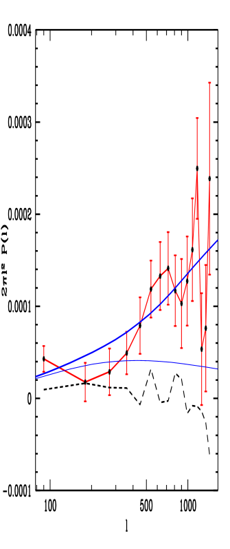
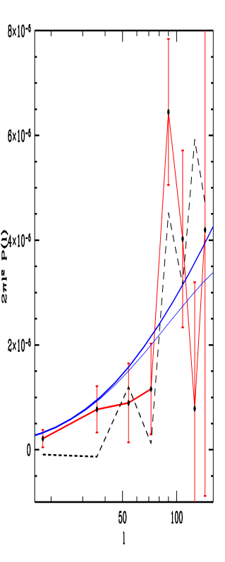
Figure 1: 2-d power spectrum reconstruction of filled 1 square degree field (left) and $100$ square degree sparsely sampled field (right). The points with error bars connected with the line are the estimators, the thick solid line is the input power spectrum, thin solid line is the corresponding linear power spectrum and dashed line is the reconstructed power spectrum of the $45^{\circ}$ rotated data.

We also tried the 3-d power spectrum estimation using the approach outlined in section 2.3. The results for the 1 square degree filled and 100 square degree sparse survey corresponding to examples in figure 1 are shown in figure 2. We show the results for the convolved power spectrum and individual estimates are strongly correlated. This, logarithmic binning and the use of logarithmic scale make the results visually more impressive than in figure 1b, although the information content is the same. Nevertheless, the results are quite impressive and an even larger (and sparser) survey would give an even bigger reward of determining the turnover in the power spectrum quite precisely. We verified the analytic error estimates from the Fisher matrix by comparing them to Monte Carlo estimates and they agree quite well. On small scales where the nonlinear effects become important the sampling error is underestimated because we used the gaussian approximation and one has to correct for that if necessary.

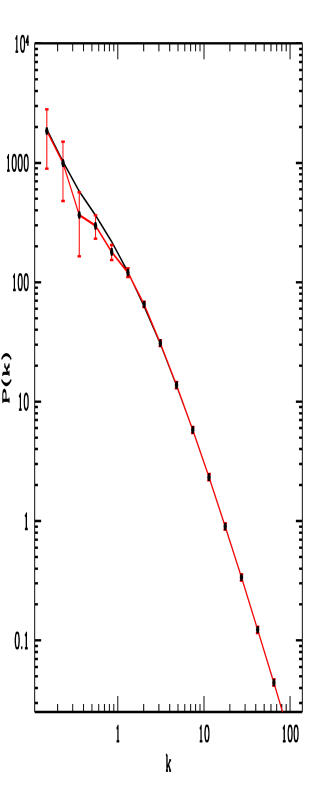
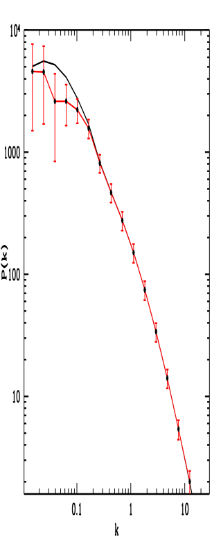
Figure 2: 3-d power spectrum reconstruction of filled 1 square degree field (left) and $100$ sparsely sampled field (right). The points with error bars connected with the line are the estimators, the thick solid line is the input power spectrum.

4 Mass density reconstruction: simulated data

In this section we apply the formalism developed in section 2 to reconstruct the projected dark matter distribution from weak lensing observations. We start with the reconstruction of large scale structure, where the techniques developed here work best. We then apply the same methods to the cluster reconstruction, pointing out its advantages and disadvantages and comparing them to other reconstructions. For this case we also generalize them to include nonlinear effects and discuss how to treat the redshift distribution of the sources. We will assume throughout this section that the power spectrum of the data is known in advance, using the techniques developed in section 3. The power spectrum is only known where the signal exceeds the noise, beyond that one has to assume its form by parametrizing it with a power law. We will use in the applications the actual power spectrum obtained from the simulated data directly. This of course cannot be obtained with the real data, but it turns out that in practice the reconstruction is not very sensitive to this, because the spectral index of the data power spectrum differs significantly from the noise spectral index 0 and so the only important parameter is the scale where the signal power spectrum exceeds the noise. Because we are expanding the data with modes that have periodic boundary conditions in a box it is better to use a somewhat larger box than the size of the observed field and zero pad the rest. For the examples here we used 10% padding on each side and in most cases this eliminated the spurious effects associated with periodic boundary conditions. If this is not sufficient one can always increase the size of zero padded area.

4.1 Large Scale Structure Reconstruction

We begin with the reconstruction of large scale structure. For this purpose we generated a projected density map from an N-body simulation. The simulated data in figure 3 were obtained by randomly placing $2\times 10^{5}$ galaxies on a 1 square degree field. Upper left panel of figure 3 shows the input data, which have a lot of small scale structure. Smoothing the input data at the scale where signal power spectrum equals the noise power spectrum produces upper right panel of figure 3. WF reconstruction is given in lower left panel of figure 3. We see that WF strikes the balance between the resolution and signal to noise ratio. The reconstruction is heavily smoothed because of the low signal to noise on small scales. On the other hand, most of the reconstructed structures are real (compare upper right with lower left panel), because WF preferentially keeps the modes that are above the noise. WF is thus particularly useful for identifying the large scale structures, such as filaments or superclusters in the data. Rotation of the galaxies by $45^{\circ}$ eliminates most of the signal and the reconstructed field is now significantly lower than the typical structures in the reconstruction, as given in lower right panel of figure 3. This does not however completely eliminate the signal, because as discussed in section 3 aliasing of power from the gravity mode into the vorticity mode makes the latter nonvanishing even in the limit of small noise. The effect is rather small because of the large number of background galaxies, but would be more important if sampling was sparse.

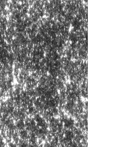
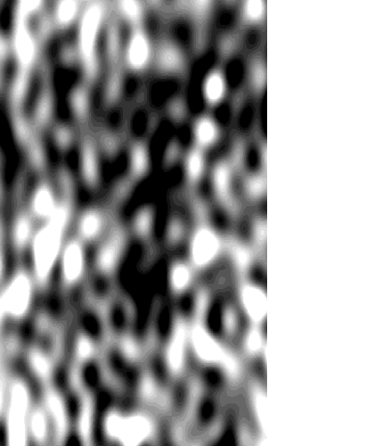
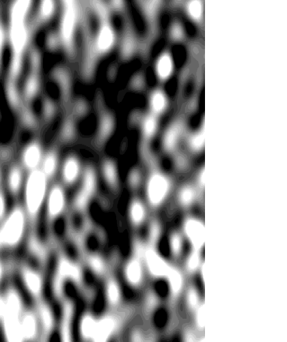
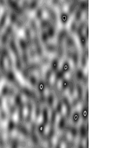
Figure 3: Reconstruction of a random portion of the sky. The sidelength is 1 degree and $2\times 10^{5}$ randomly generated galaxies have been used for reconstruction. Top left are input data, top right smoothed input data, bottom left WF reconstruction and bottom right $45^{\circ}$ rotation test. Most reconstructed structures have surface density of a few percent.

4.2 Cluster Reconstruction

The methods we developed in this paper are optimal for gaussian random fields, but they can also be applied to nongaussian situations, such as cluster reconstruction from weak lensing. In this case WF by definition still minimizes the variance in the class of linear estimators as shown in section 2.1 and so remains a useful reconstruction technique. To test it we apply it to reconstruct a massive cluster obtained from an N-body simulation (figure 5a). We have rescaled the projected mass density of the cluster in units of critical density, so that it is nearly critical. The cluster core is very concentrated and shows double nucleus structure. The comoving size of the box is 3.2$h^{-1}$Mpc and we will take the area to be 10’ across with 5000 galaxies in it. In this subsection we want to compare the reconstruction properties of various filtering methods and we will ignore the nonlinear corrections. Those will be addressed in the next subsection.

There exist a number of cluster reconstruction techniques in the literature. Squires & Kaiser (1996) present a comprehensive review of most of these and conclude that their so-called maximum probability model is the best in the sense that it has the least amount of long-wavelength noise in the noise power spectrum. This is not surprising, since their model is identical to WF (in Fourier space), except that they advocate the prior power spectrum to be white noise with adjustable amplitude. The latter was taken to be larger than the noise, so that it does not suppress the modes on any scale (the only reason Squires & Kaiser (1996) add the theoretical prior is to regularize the inversion of matrix $D$). Because for long wavelength modes the actual signal is typically larger than the noise (as shown in figure 4 for the cluster used here) the results will be similar to WF and both methods will reconstruct long wavelength modes without any suppression. However, on scales where the power spectrum drops below the noise the two methods differ: white noise prior does not filter the modes and is reconstructing mainly noise, while WF suppresses the modes, returning zero in the regions of low signal to noise. This is what one expects from a minimum variance method, since zero deviates from the true field less than the random noise does when the power spectrum of the latter exceeds the former. This is shown in figure 4 for the simulated cluster. For short wavelengths white noise prior is no longer optimal in the sense of minimizing the variance and so in this sense WF is a minimum variance reconstruction among linear estimators even for a cluster. But as we show next this may not be the most desirable feature in the reconstruction and other methods (such as the one investigated by Seitz and Schneider 1996) may result in a better overall reconstruction.

Because the power spectrum has less power on small scales than the white noise one expects WF to result in a smoother reconstruction than the one assuming white noise as a theoretical prior. WF reconstruction of the cluster is shown in upper right panel of figure 5 and indeed is rather smooth compared to the white noise prior WF reconstruction. Note that the uniform weighting with variable theoretical variance (equation 13) shown in the middle left panel of figure 5 gives almost identical results, but is much easier to compute. WF reconstruction shows a clear signature of the cluster above the background or above the $45^{\circ}$ rotation reconstruction in the middle right panel of figure 5, which does not show any evidence of a cluster. The noise is mostly eliminated from the map and most of the large structures one sees are real. These properties make WF to be a useful method even for cluster reconstruction. However, there is a high price to pay for this. By suppressing the small scale modes and so the noise across the field WF also suppresses the central peak of the cluster. Some amount of smoothing is of course inevitable if the data do not have sufficient resolution, but WF tends to heavily smooth the data by suppressing all the small scale modes, regardless of their position. The nongaussian nature of the cluster center may give sufficient signal to noise to reconstruct it, but because all of the power on small scales is concentrated in this small region it may not give statistically significant excess above the noise in the power spectrum analysis. This in fact becomes exacerbated as we increase the area of the reconstruction, because by attempting to reconstruct the whole area (with no power on small scales over most of the region) WF will further suppress the central part of the cluster. For some applications one may be interested more in the central part of the cluster and willing to accept higher levels of noise at the outskirts of the cluster in which case WF will not be ideal method.

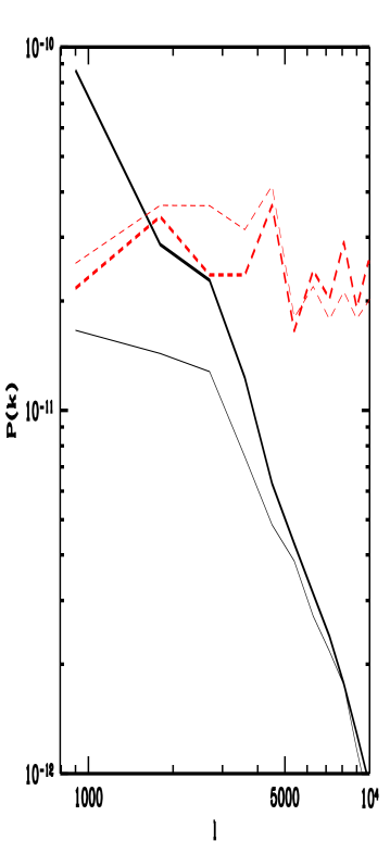
Figure 4: Power spectrum of signal (thick solid curve) and noise (thick dashed curve), obtained by computing the power spectrum with only cluster or only noise, respectively. Only for long wavelength modes signal exceeds the noise. Thin lines give the power spectrum of residuals, (the difference between the true and reconstructed modes) for WF (solid) and white noise prior WF (dashed). The two have similar noise properties for long wavelength modes, while for short wavelengths white noise prior gives much larger noise variance and reduces to the noise power spectrum, because the true modes are small. Conversely for WF the power spectrum of residuals reduces to the signal power spectrum on small scales because the reconstructed modes are small.

For cluster reconstruction it is therefore worth extending the family of linear estimators to make the prior power spectrum a free parameter. One example in this class is white noise prior advocated by Squires & Kaiser (1996), which can reconstruct the structure on small scales. It should be stressed that with white noise prior one still has to impose a high frequency cutoff, otherwise the noise on small scales completely dominates the reconstruction. The way Squires & Kaiser (1996) impose this is by restricting themselves to a small number of modes in the expansion, although the actual number was left unspecified. This method therefore amounts to a simple low-pass filtering, where the filter is a step function, as opposed to the WF, where the filter is more gradual and depends on the actual signal to noise ratio in the power spectrum of the data. If we extend the filtering scale beyond the scale where signal and noise power spectra are equal we obtain the reconstruction shown in lower right panel of figure 5 for one particular choice of cutoff in $k$. Most of the reconstructed structure on small scale is noise, which clearly does not minimize the variance as defined in equation (12) and so is not optimal in this sense. On the other hand, the central peak of the cluster is now significantly higher and its detection is more significant than in the case of WF. In this case reconstruction with smaller filtering scale may be more acceptable, despite being significantly noisier. Nonlinear methods such as maximum entropy method (Narayan & Nityananda (1986)) are likely to do even better in such applications. Note that the spike at the corner of the white noise prior reconstruction is an artifact of the periodic boundary conditions and would be eliminated if one used 20% zero padding on each side of the box. This example shows that one has to be careful about the size of the zero padding area, which will be somewhat dependent on the type of the filter one is using.

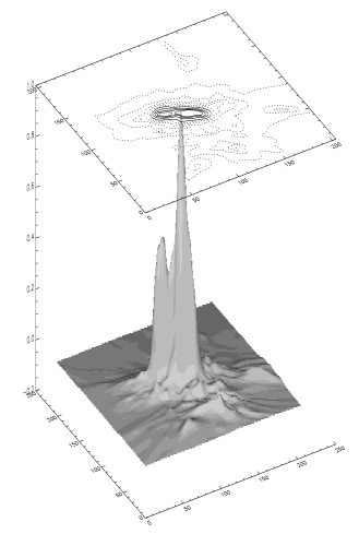
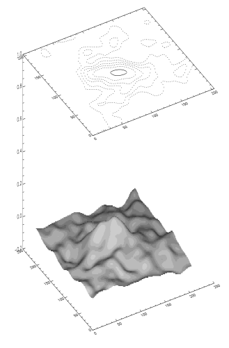
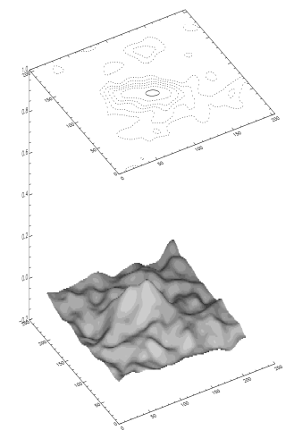
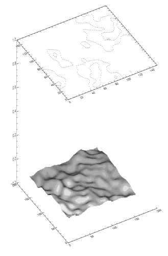
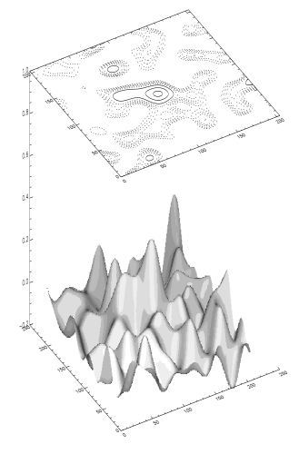
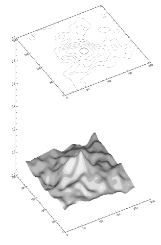
Figure 5: The dimensionless surface mass density $\kappa$ for the simulated cluster. The sidelength is 10’ and 5000 randomly generated galaxies have been used for reconstruction. The contour levels are 0.1,0.2,0.3,0.4 (solid) and 0.01,0.03,0.05,0.07 (dashed). From top left to bottom right the plots are: input data, WF reconstruction, WF reconstruction with uniform weighting approximation, $45^{\circ}$ rotation test, white noise prior WF reconstruction and WF nonlinear reconstruction. WF heavily smooths the data, because the cluster is only a small part of the observed region and does not add a lot of power to the power spectrum.

WF reconstruction is also not unique and changes with the size of the observed area. If we reduce the size then the cluster becomes more important and the contribution from nongaussian modes to the power spectrum can dominate over the noise to smaller scales than in previous example, resulting in keeping more small scale modes in the reconstruction. An example of this is shown in figure 6, where we increased the physical size of the cluster by a factor of two, keeping the other parameters unchanged. This enhanced the signal power spectrum and added the small scale structure to the reconstruction. Most of this structure outside the cluster is noise, but now this noise does not dominate the power spectrum and the minimum variance estimator is allowed to keep this structure and reconstruct the true structure in the center as well. It is clear from this discussion that WF is no longer optimal for every application and can only be treated as one example in a wider class of linear filters. For a conservative reconstruction of the whole measured area WF will in general outperform other methods. Other low-pass filters may however be more appropriate for more specific applications. We may conclude that using the measured power spectrum from the data in WF is a useful starting procedure, which should be supplemented by other linear filters by varying the prior power spectrum. Nonlinear methods, such as maximum entropy method, may provide an even better reconstruction of strongly nongaussian and point-like structures.

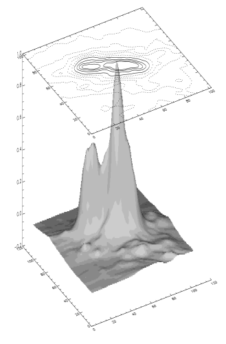
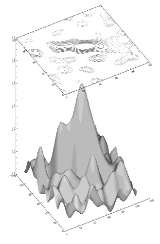
Figure 6: Same cluster as in figure 3.1 assuming it is twice larger in the sky. The sidelength, number of galaxies and contour levels are the same as in figure 3.1. Left is the input surface density, right the nonlinear WF reconstruction. In this case WF smooths the data less than in figure 3.1, because the cluster is a dominant part of the observed region and the nongaussian small scale modes add a lot of power to the power spectrum.

4.3 Nonlinear effects

So far we ignored the term $1-\kappa$ in relating observed ellipticity to underlying shear field by assuming that $\kappa$ is small. When the clusters are nearly critical, such as in the core of the cluster we used above, the corrections become important and have to be included. Because the final result of the reconstruction is convergence $\kappa$ one can include the correction using an iterative scheme: one first reconstructs $\kappa$ using equation (13) ignoring the correction and in the next step one uses the value of reconstructed $\kappa$ to obtain the components of the shear $\gamma_{i}$ from the observables $e_{i}$

$$\gamma_{i}(\hbox{\boldmath{$\theta$}})=e_{i}(\hbox{\boldmath{$\theta$}})/[1-\hat{\kappa}(\hbox{\boldmath{$\theta$}})].$$ (35)

These corrections tend to suppress the reconstructed convergence, because the shear is reduced for the same measured ellipticity. A similar iterative scheme has been proposed by Seitz & Schneider (1995). Assuming that $\hat{\kappa}(\hbox{\boldmath{$\theta$}})$ is not close to unity then the error on the shear will continue to be dominated by the error on ellipticity $e_{i}$ and one can repeat the analysis as before with new values of the shear. Otherwise one can improve this by adding additional term to the error matrix that corresponds to the error contribution from the reconstructed convergence, which is given by (equation 14)

$$\langle[\hat{\kappa}(\hbox{\boldmath{$\theta$}})-\kappa(\hbox{\boldmath{$\theta$}})][\hat{\kappa}(\hbox{\boldmath{$\theta$}})-\kappa(\hbox{\boldmath{$\theta$}})]^{{\dagger}}\rangle=\hbox{\boldmath{$R$}}_{\kappa}\hbox{\boldmath{$D$}}^{-1}\hbox{\boldmath{$R$}}_{\kappa}$$ (36)

and properly add the two error contributions. If the cluster contains a critical line where $|\det\Phi|=0$ then inside outer line (but outside inner critical line) one should replace $e_{i}$ with $e_{i}/e^{2}$ (Kaiser (1995)) and one way to handle this case is to identify the critical lines at the previous iteration, replace $e_{i}$ with $e_{i}/e^{2}$ where necessary and repeat the iteration until the convergence. We implicitly assumed that the zero point of convergence is known, which is something that cannot be reconstructed from the ellipticity measurements alone. When reconstructing LSS this will not be a major problem, since the mean convergence fluctuates by a few percent at most (the power from the modes larger than the size of the field is small). One can thus impose the mean convergence to vanish across the survey by setting the unreconstructed $k=0$ mode to zero. For cluster reconstruction it is more appropriate to set the zero point so that the convergence at the outskirts of the cluster is zero and this is somewhat more problematic when the cluster extends to the edge of the field. For the example we used in this paper this is not so much of a problem, as one can separate the cluster from the surrounding area where the mean convergence should be small. One can in fact completely avoid this problem by using a local relation between derivatives of shear and convergence (Kaiser (1995); Seitz & Schneider (1996)), although it does not appear straight-forward to implement this in the methods developed here.

4.4 Redshift distribution of the sources

In section 3 we discussed how to handle the redshift distribution of the sources for the power spectrum estimation. One approach was to divide the galaxies into bins localized in distance and perform the analysis on each of these. The same approach should also be used for LSS reconstruction, because the deflections come from a broad region along the line of sight and can only be determined in a statistical sense. In the case of cluster reconstruction the situation differs from LSS because the deflector is in a single lens plane and the distance to it is assumed to be known. Instead of using convergence $\kappa$, which depends on the lens and source positions, it is better to model directly the surface density $\Sigma$, which is a physical quantity independent of the redshift distribution. It is related to the convergence via the relation

$$\kappa={\Sigma\over\Sigma_{{\rm crit}}},\,\,\,\Sigma^{-1}_{{\rm crit}}(\chi_{s},\chi_{l})=4\pi Ga(\chi_{l}){r(\chi_{l})r(\chi_{s}-\chi_{l})\over r(\chi_{s})},$$ (37)

where $\chi_{s}$ and $\chi_{l}$ are the radial comoving distances to the source and lens, respectively. When the sources are all at the same distance one can work with $\kappa$ and then obtain $\Sigma$ using the above relation. When the sources are not at the same distance then $\kappa$ changes with $\chi_{s}$ for the same surface density $\Sigma$. The observable $e_{i}$ can be expressed directly in terms of $\Sigma$ in analogy to equations (8), (35) as

$$e_{i}(1-\Sigma/\Sigma_{{\rm crit}})\Sigma_{{\rm crit}}=\hbox{\boldmath{$R$}}\tilde{\hbox{\boldmath{$\Sigma$}}}+\hbox{\boldmath{$n$}}.$$ (38)

Because the galaxy distance is not known $\Sigma_{{\rm crit}}$ is a stochastic variable and can be treated as the estimate plus additional noise term. Assuming each galaxy has a known probability distribution of distances $W_{i}(\chi)$ (in the absence of any distance information this is just the overall galaxy distribution), we can define the mean critical density

$$\bar{\Sigma}^{-1}_{i,{\rm crit}}=\int d\chi_{s}W_{i}(\chi_{s})\Sigma^{-1}_{{\rm crit}}(\chi_{s},\chi_{l})$$ (39)

and the dispersion around it

$$\sigma^{2}_{i}(\Sigma^{-1}_{{\rm crit}})=\int d\chi_{s}W_{i}(\chi_{s})(\Sigma^{-1}_{{\rm crit}}(\chi_{s},\chi_{l})-\bar{\Sigma}^{-1}_{{\rm crit}})^{2}.$$ (40)

For each galaxy we use the mean critical density $\bar{\Sigma}_{i,{\rm crit}}$ in equation (38) as the estimate and the dispersion $\sigma^{2}_{i}(\Sigma_{{\rm crit}})$ as an additional source of error in the observable $e_{i}(1-\Sigma/\Sigma_{{\rm crit}})\Sigma_{\rm crit}$. This additional noise term will be negligible for clusters at low $z$ (where $\Sigma_{{\rm crit}}$ is rather insensitive to the redshift distribution of sources). Even for high $z$ clusters this error is typically subdominant compared to the error on the ellipticity if the convergence is small. The only case when this error becomes important is for clusters that are close to critical, where the uncertainty on $\Sigma_{{\rm crit}}$ in the term $1-\Sigma/\Sigma_{{\rm crit}}$ of equation (38) is amplified and can dominate over the ellipticity error, in which case we can add this error to the overall error budget of that galaxy. An alternative treatment of this problem has been discussed by Seitz & Schneider 1996b for the case when the overall probability distribution of galaxy redshifts is given. The nice feature of our approach is that the mean distance and its error can be attached to each galaxy individually, which can take advantage of the multicolor photometric information. By assigning to each galaxy its photometric redshift and the corresponding error estimate we can compute for each galaxy separately its critical density and the dispersion around it. Another example when this is important is when the measurement errors increase for fainter and presumably more distant sources. In this case the more nearby galaxies carry more weight than expected from their number density and one can correct for this by assigning to each galaxy a mean distance according to its observed flux.

5 Discussion

In this paper we address the question of optimal power spectrum estimation and projected mass density reconstruction from weak lensing data. We show that for gaussian random processes both have a well defined answer, which are in fact related and can be obtained from the same calculation. For the power spectrum the final answer is given by the unbiased estimator and its covariance matrix (which also acts as a window function). The estimator is equivalent to the maximum likelihood method, but is significantly faster to compute. The covariance matrix of estimators includes the contributions from noise, sampling variance and aliasing. It is possible to invert from the 2-d power spectrum or to compute directly from the data the 3-d power spectrum, which will also be unbiased and minimum variance. Finally, if we have distance information for the galaxies based on their photometric properties we can solve for both the power spectrum and its time dependence. The method can be used in the nonlinear regime, where it remains unbiased, but one has to compute the covariance matrix of the estimators, which now depend also on the reduced four point correlator. This can be either estimated from the data themselves, obtained from N-body simulations or computed using perturbation theory or hierarchical scaling relations. It is important to realize that even though the estimators were derived from the maximum likelihood method, the final result is always a weighted quadratic average of the data, where the weighting is the inverse of covariance matrix. This is the most expensive part of the calculation and can be replaced by some simpler weighting if necessary, such as uniform or inverse noise weighting. Even in this case the method will remain unbiased and will in fact remain close to optimal on small scales. Similarly, if one wants to parametrize the power spectrum with some other parameters (such as its amplitude and slope) one can derive unbiased quadratic estimators specifically tailored for those parameters instead of going through the power spectrum. This is however not necessary, since in the process of reducing the data to the power spectrum no information has been lost if minimum variance estimator has been used.

Another topic of interest that we did not discuss in detail here is the question of optimal measurement of higher moments. One attempt how to measure these has been presented by Schneider et al. (1997) using mass aperture statistic. As mentioned in the introduction this statistic uses the tangential component of the shear to obtain a quantity that is a scalar (as opposed to shear which is a tensor), which is needed to define a nonvanishing third moment in real space. Alternative way to obtain a scalar quantity is to reconstruct the convergence in Fourier space as done in this paper. Within the context of the methods presented here the general strategy for determining the higher moments is in fact similar to the one leading to the minimum variance power spectrum methods, at least in the limit where the higher moments are small. One first multiplies the measurements with the inverse of correlation matrix. This is just a consequence of inverse variance weighting: if a given measurement has a large measurement error or it is strongly correlated with neighbouring points then it has to be downweighted, because it does not add new information to the data. On small scales this weighting reduces to the simple uniform weighting as discussed in section 2. One then projects the data to Fourier space to make a scalar quantity. Because we reconstruct the Fourier modes first one can attempt to measure higher order moments directly in Fourier space (e.g. bispectrum for the case of three-point statistic) and this has some nice advantages (e.g. Scoccimarro et al. (1997)). One can for example average over all triple products $\hat{\tilde{\kappa}}(\hbox{\boldmath{$l$}}_{1})\hat{\tilde{\kappa}}(\hbox{\boldmath{$l$}}_{2})\hat{\tilde{\kappa}}(\hbox{\boldmath{$l$}}_{3})$ with $\hbox{\boldmath{$l$}}_{1}+\hbox{\boldmath{$l$}}_{2}+\hbox{\boldmath{$l$}}_{3}=0$, keeping the shape of the triangle the same and then vary this as a function of scale and angle between the wavevectors. As for the case of the power spectrum one has to compute the window for this statistic to make the estimator unbiased and to place errors on the estimates. Alternatively, one can transform $\tilde{\hbox{\boldmath{$\kappa$}}}$ back to real space by applying $\hbox{\boldmath{$R$}}_{\kappa}$ operator to obtain a real space quantity that is a scalar, which can then be used to measure its skewness as a function of smoothing radius (filtering scale). Because all the operations are linear on the data one can obtain the covariance matrix of the estimates and compute the window function needed to make the estimator unbiased and provide error estimate.

For projected mass density reconstruction the WF method investigated here works best on large scales, where the distribution is close to gaussian. In that case WF preferentially keeps the structure that is above the noise and filters out scales that are noise dominated. To apply WF one has to compute the power spectrum on the data first using the methods discussed above. When the structures become nonlinear WF remains a useful reconstruction technique and still minimizes the variance in the class of linear estimators, but tends to oversmooth the data in very dense regions such as clusters. In that case it should be supplemented with linear filtering with a shorter smoothing scale or with one of the nonlinear methods, depending on the particular application one has in mind. This will be particularly important if one is searching for clusters in a random survey, where their positions are not given in advance and one wants to maximize the signal to noise for detecting such structures.

References

- Baugh & Efstathiou (1994)
- (2) augh, C. M., & Efstathiou, G. 1994, MNRAS, 267, 323
- Bernardeau et al. (1997)
- (4) ernardeau, F., van Waerbeke, L., & Mellier, Y. 1997, A&A, 322, 1
- Blandford et al. (1991)
- (6) landford, R. D., Saust, A. B., Brainerd, T. G., & Villumsen, J. V. 1991, MNRAS, 251, 600
- Bond, Knox & Jaffe (1997)
- (8) ond, J. R., Knox, L., & Jaffe, A. H. 1997, astro-ph/9708203
- Bond, Efstatiou & Tegmark (1997)
- (10) ond, J. R., Efstathiou, G., & Tegmark, M. 1997, astro-ph/9702100
- Bunn, Hoffman & Silk (1995)
- (12) unn, E. F., Hoffman, Y., & Silk, J. 1996, ApJ, 464, 1
- Connolly et al. (1995)
- (14) onnolly, A. J., Scabai, I., Szalay, A. S., Koo, D. C., Kron, R. C., & Munn, J. A., AJ, 110, 2655
- Dekel & Lahav (1997)
- (16) ekel, A., & Lahav, O. 1997, in preparation
- Fort & Mellier (1994)
- (18) ort, B., Mellier, Y. 1994, A&A Review, R, 239, 292
- Gaztañaga & Baugh (1997)
- (20) aztañaga, E., & Baugh, C. M. (1997), MNRASin press, astro-ph/9704246
- Górski (1994)
- (22) órski, K. M. 1994, ApJ, 430, L85
- Gunn (1967)
- (24) unn, J. E. 1967, ApJ, 147, 61
- Jungman et al. (1996)
- (26) ungman, G., Kamionkowski, M., Kosowsky, A. & Spergel, D. N. 1996, Phys. Rev. D, 54, 1332
- Hamilton et al. (1991)
- (28) amilton, A. J. S., Kumar, P., Lu, E., & Matthews, A. 1991, ApJ, 374, L1
- Hamilton (1997) Hamilton, A. J. S. 1997, MNRAS, 289, 285
- Heyl et al. (1995)
- (31) eyl, J. S., Cole, S., Frenk, C. S., & Navarro, J. F. 1995, MNRAS, 274, 755.
- Jain & Seljak (1997)
- (33) ain, B., & Seljak, U. 1997, 484, 560
- Kaiser (1992)
- (35) aiser, N. 1992, ApJ, 388, 272
- Kaiser (1995)
- (37) aiser, N. 1995, ApJ, 439, L1
- Kaiser (1997)
- (39) aiser, N. 1997, ApJ, in press, astro-ph/9610120
- Kaiser et al. (1994)
- (41) aiser, N., Squires, G., Fahlman, G. & Woods, D. 1994, in: Clusters of Galaxies, eds. F. Durret, A. Mazure & Tran Thanh Van, Editiones Frontieres
- Kendall & Stuart (1969)
- (43) endall, M. G., & Stuart, A. 1969, ‘The Advanced Theory of Statistics’, Volume II (Griffin, London)
- Kochanek (1990)
- (45) ochanek, C. S. 1990, MNRAS, 247, 135
- Miralda-Escude (1991)
- (47) iralda-Escude, J. 1991, ApJ, 380, 1
- Narayan & Nityananda (1986)
- (49) arayan, R., & Nityananda, R. 1986, ARA&A, 24, 127
- Oh, Spergel & Hinshaw (1997)
- (51) h, S. P., Spergel, D. N., & Hinshaw, G. 1997, in preparation
- Rybicki & Press (1992)
- (53) ybicki, G., & Press, W. H. 1992, ApJ, 398, 169
- Scoccimarro et al. (1997)
- (55) coccimarro, R., Colombi, S., Fry, J. N., Frieman, J. A., Hivon, E., & Melott, A. 1997, astro-ph/9704075
- Schneider et al. (1997)
- (57) chneider, P, van Waerbeke, Jain, B., & Kruse, G. 1997, astro-ph/9708143
- Seitz & Schneider (1995)
- (59) eitz, C., & Schneider, P. 1995, A&A, 297, 287
- Seitz & Schneider (1996)
- (61) eitz, S., & Schneider, P. 1996, A&A, 305, 383
- (62)
- (63) eitz, C., & Schneider, P. 1996, A&A, 318, 687
- Seljak (1996)
- (65) eljak, U. 1996, ApJ, 463, 1
- Seljak (1997)
- (67) eljak, U. 1997, submitted to ApJ, astro-ph/9710269
- Squires & Kaiser (1996)
- (69) quires, G., & Kaiser, N. 1996, ApJ, 473, 65
- Strauss & Willick (1995)
- (71) trauss, M. A., Willick, J. A. 1995, Physics Reports, 261, 271
- Stebbins (1996)
- (73) tebbins. A. 1996, preprint astro-ph/9609149
- Tegmark (1997)
- (75) egmark, M. 1997, Phys. Rev. D, 55, 5895
- Tegmark, Taylor & Heavens (1997)
- (77) egmark, M., Taylor, A., & Heavens, A. 1997, ApJ, 480, 22
- Villumsen (1996)
- (79) illumsen, J. V. 1996, MNRAS, 281, 369
- Zaldarriaga, Spergel & Seljak (1997)
- (81) aldarriaga, M., Spergel D. & Seljak, U. 1997, ApJ, 488, 1
- Zaroubi, Hoffman, Fisher & Lahav (1995)
- (83) aroubi, S., Hoffman, Y., Fisher, K., B., & Lahav, O. 1995, ApJ, 449, 446