OU-TAP 62
Effects of merging histories on angular momentum distribution of dark matter haloes

Abstract

The effects of merging histories of proto-objects on the angular momentum distributions of the present-time dark matter haloes are analysed. An analytical approach to the analysis of the angular momentum distributions assumes that the haloes are initially homogeneous ellipsoids and that the growth of the angular momentum of the haloes halts at their maximum expansion time. However, the maximum expansion time cannot be determined uniquely, because in the hierarchical clustering scenario each progenitor, or subunit, of the halo has its own maximum expansion time. Therefore the merging history of the halo may be important in estimating its angular momentum. Using the merger tree model by Rodrigues & Thomas, which takes into account the spatial correlations of the density fluctuations, we have investigated the effects of the merging histories on the angular momentum distributions of dark matter haloes. It was found that the merger effects, that is, the effects of the inhomogeneity of the maximum expansion times of the progenitors which finally merge together into a halo, do not strongly affect the final angular momentum distributions, so that the homogeneous ellipsoid approximation happens to be good for the estimation of the angular momentum distribution of dark matter haloes. This is because the effect of the different directions of the angular momenta of the progenitors cancels out the effect of the inhomogeneity of the maximum expansion times of the progenitors.

The contribution of the orbital angular momentum to the total angular momentum when two or more pre-existing haloes merge together, was also investigated. It is shown that this contribution is more important than that of the angular momentum of diffuse accreting matter to the total angular momentum, especially when the mergers occur many times.

1 INTRODUCTION

Galaxy formation is one of the most important problems in astrophysics. In general, it includes different physical processes such as the evolution of cosmological fluctuations, star formation, heating processes of baryonic gas from supernovae, dynamical and chemical evolution of gas, etc. Hence it is difficult to attack the problem of the formation and evolution of galaxies in a way that connects all of the complicated physical processes.

One of the important keys to understanding galaxy formation is the angular momentum of dark matter haloes. For example, there is a strong correlation between the angular momentum and the morphology of galaxies. The mean value of the angular momentum of ellipticals is much smaller than that of spirals. Thus we may expect to understand the origin of the morphological distinction from analysis of the angular momentum. In the standard model, it is considered that dark matter dominates in our Universe and that galaxies and clusters of galaxies have been formed by the gravitational growth of small initial density fluctuations. The dark matter has collapsed and virialized by self-gravitational instability into objects which are called ‘dark matter haloes’ or ‘dark haloes’. The large haloes are generally considered to have been formed hierarchically by the clustering of smaller ones (so-called ‘hierarchical clustering’). During this process, each dark halo obtains its angular momentum by tidal forces (Hoyle 1949; Peebles 1969; White 1984; Barnes & Efstathiou 1987). Also, some properties of the baryonic component of galaxies e.g. morphologies, surface brightness and so on, have been discussed as a function of angular momentum of dark haloes (e.g., Dalcanton, Spergel & Summers 1997; Jimenez et al. 1997; Mo, Mao & White 1998).

Doroshkevich (1970) and White (1984) found that the angular momentum evolves proportionally to $t$ ($t$ is the cosmic time) during the linear regime, considering the initially homogeneous density ellipsoid as a proto-object in the Einstein-de Sitter universe. This prediction has been confirmed by the N-body simulations by White (1984) and Barnes & Efstathiou (1987). It should be noted that White (1984) did not consider whether the dark matter in the region under consideration would in fact grow into a collapsed object or not in his analytical prediction.

In the analysis of the evolution of the angular momentum of a proto-object, it is assumed that the dark matter around a density peak maximum collapses into a halo (Hoffman 1986, 1988; Ryden & Gunn 1987; Ryden 1988; Caimmi 1989; Quinn & Binney 1992 and Eisenstein & Loeb 1995a, b). The angular momentum distributions were derived analytically by Heavens & Peacock (1988), and Catelan & Theuns (1996a, b). They used the peak formalism of Gaussian random fields (Peacock & Heavens 1985; Bardeen et al. 1986), in order to analyse statistically a density profile around the density peak maximum. Catelan & Theuns also considered the case of non-Gaussian initial conditions (Catelan & Theuns 1997). Susa, Sasaki & Tanaka investigated the angular momentum distribution by using the Press-Schechter formalism (Press & Schechter 1974) instead of the peak formalism.

It should be noted that when the distribution of the angular momentum was derived, there was assumed that an ‘object’ is the initially homogeneous density ellipsoid and that the acquisition of the angular momentum halts at the maximum expansion time of the object (Heavens & Peacock 1988; Catelan & Theuns 1996a, b). The maximum expansion time is usually estimated from the averaged density contrast of the object by assuming spherically symmetric collapse. In spherical collapse, the averaged linear density contrast of the object reaches to $1.05$ at the maximum expansion time (e.g. Peebles 1993). However, in the hierarchical clustering scenario, small objects collapse firstly. Some of the small objects may then merge together, leading to the present-time large halo. It is general in this scenario that the acquisition of the angular momentum of a dominant proto-object of a halo may halts earlier than the maximum expansion time estimated through the averaged density contrast of the present-time halo. Hence, if we believe in the merging history of the proto-objects, then we should take into account the halting time of each proto-object, a contribution of the orbital angular momentum of the merging proto-object, and the angular momentum of the accreting matter.

Merging history models of dark haloes have been used for the semi-analytical methods of galaxy formations (Cole & Kaiser 1988; Kauffmann & White 1993; Rodrigues & Thomas 1996; Roukema et al. 1997). Cole & Kaiser developed the block model, considering the one-point distribution function of density fluctuations. Therefore spatial correlations of the density fields were not taken into account. Kauffmann & White (1993) extended the Press-Schechter formalism and constructed the merging histories by coupling this formalism with the Monte Carlo method. The extension in question is mainly based on the results of Bower (1991). Kauffmann & White (1993) have utilized the one-point distribution function as well. On the other hand, Yano, Nagashima & Gouda (1996) have shown that the spatial correlation of the density field is important when calculating mass function of dark haloes. The analytically derived mass function accounting explicitly for the two-point correlation function, differs significantly from that found by the Press-Schechter mass function. So we believe that the merging histories should also include spatial information. Rodrigues & Thomas (1996) constructed the merging history model (which we call ‘the merging cell model’, for convenience), including the information on the spatial correlations. In the merging cell model, the random Gaussian density fluctuation field is realized on spatial grids as in the construction of the initial conditions of N-body simulations. Therefore this model includes, naturally, information on the spatial correlation. Then, by finding the collapsed region whose linear density contrast, $\delta$, averaged over the region is $\delta_{c}=1.69$ ($\delta_{c}$ is the critical density contrast for collapse, see, e.g., Peebles 1993), we can construct merger trees. We expect that this model is more realistic and useful in describing the galaxy formations although a spherical collapse of each block is assumed. Nagashima & Gouda (1997) have analysed this merging cell model by comparing the mass functions given by the merging cell model with the mass functions by Yano, Nagashima & Gouda (1996). They found that both types of the mass functions are in good agreement.

In this paper, using the merging cell model, we calculate both the density fields and the velocity fields in order to estimate the angular momentum distribution of dark haloes. In a similar way to the previous analytical work (Heavens & Peacock 1988; Catelan & Theuns 1996a, b), the initial angular momentum of each halo is calculated through the velocity field, then the angular momentum of each halo is evolved proportionally to the cosmic time $t$. Since the overdensity of each halo is known, we can estimate its maximum expansion time. By using this time, we compute the angular momentum of the halo. When a merger between the haloes occurs, we investigate the spins and the orbital angular momentum of these haloes around the centre-of-mass of a larger new common halo, and the angular momentum of the matter being accreted into the new halo. The sum of these angular momentum components is the spin of the new halo. This process is repeated when the mergers occur. It should be noted that the block model and the extension of the Press-Schechter formalism cannot deal with angular momentum, because these models ignore the velocity field structures.

To compare our method with the previous work, we also calculate the angular momentum of homogeneous density haloes by smoothing density contrasts in each region occupied by haloes at the present epoch. In this way we investigate the effects of the merging histories by showing the angular momentum distribution of dark haloes.

Our aim is to clarify the physical effects of the merging histories of dark haloes, namely, the effects of the difference in the maximum expansion times and the difference in the directions of the angular momenta of the proto-objects, that is, the subunits of the haloes. An advantage of our method is that it makes available a qualitative analysis of the acquisition of angular momentum. Of course, we must perform N-body simulations in order to understand the process quantitatively (Efstathiou & Jones 1979; Barnes & Efstathiou 1987; Warren et al. 1992; Lemson & Kauffmann 1997), but our calculations require less computing time than do N-body simulations. Therefore, we can investigate many model parameters for a short time. We believe that the semi-analytical methods are complementary to N-body simulations.

In Section 2, previous analytical work is reviewed briefly. In Section 3, the merging cell model is characterized. In Section 4, the method of calculating the angular momenta of haloes in the merging cell model is shown. In Section 5, we consider the angular momentum distribution. We show the merger effects as well as the role of the orbital angular momentum of the merging objects in their common halo. Section 6 is devoted to conclusions and discussion.

2 TIME DEPENDENCE OF ANGULAR MOMENTUM

In this section, we review the evolution of angular momentum according to the White’s method (White 1984). The notations are almost the same as in Catelan & Theuns (1996a).

The angular momentum ${\bf L}$ of an object occupying the volume $V$ in the Eulerian space is defined as

$${\bf L}(t)\equiv\int_{V}\rho({\bf r})({\bf r}-{\bf r}_{0}){\times}({\bf v}-{\bf v}_{0})d{\bf r},$$ (1)

where $\rho$ is the density, ${\bf r}$ is the Eulerian coordinate, ${\bf v}$ is the velocity, and the subscript $0$ denotes the centre-of-mass of the volume $V$. This transforms to the Lagrangian description,

$${\bf L} = \int_{\Gamma}\eta_{0}a^{2}\left[{\bf q}-{\bf q}_{0}+D\nabla(\phi-\phi_{0})\right]{\times}\dot{D}\nabla(\phi-\phi_{0})d{\bf q}$$ (2)

$$= \int_{\Gamma}\eta_{0}a^{2}\dot{D}({\bf q}-{\bf q}_{0}){\times}\nabla(\phi-\phi_{0})d{\bf q},$$

with $\eta_{0}=\bar{\rho}a^{3}$, where $\eta_{0}$ is the comoving mean density of the universe, $\bar{\rho}$ is the mean density of the universe, $a$ is the cosmic scale factor, ${\bf q}$ is the Lagrangian coordinate, $\phi$ is proportional to the gravitational potential in the Einstein-de Sitter universe, $D$ is the linear growth factor ($D=a$ in the Einstein-de Sitter universe), and $\Gamma$ denotes the Lagrangian volume corresponding to $V$. The dot represents time derivative, $d/dt$. In the above transformation, we use the Zel’dovich approximation (Zel’dovich 1970),

$${\bf r}(t,{\bf q})=a(t)[{\bf q}+D(t)\nabla\phi({\bf q})].$$ (3)

Thus we find the growth rate of the angular momentum as

$$L\propto a^{2}\dot{D}\propto t$$ (4)

in the Einstein-de Sitter universe.

The growth of the angular momentum halts at the maximum expansion time of the object. In the previous work, this maximum expansion time is estimated via the density contrast at a centre of the object with the Lagrangian volume $\Gamma$, which is smoothed with a filtering scale corresponding to the mass of the object. Using the spherical collapse approximation, the maximum expansion time $t_{m}$ is obtained by $t_{m}=t_{0}(1.05/\delta)^{3/2}$, where $t_{0}$ is the present time and $\delta$ is the density contrast at the centre of $\Gamma$.

Note that the above discussion is justified only when the Zel’dovich approximation is valid anywhere in $\Gamma$ until $t_{m}$. However, in hierarchical clustering scenarios, collapsed haloes cluster and grow up gradually, so that the Zel’dovich approximation in such pre-existing haloes is broken earlier than $t_{m}$ of the final collapsed halo with $\Gamma$. Therefore, we need to investigate the case in which the growth of angular momenta of the pre-existing haloes halts earlier than the maximum expansion time of the final collapsed halo which is formed via mergers of the pre-existing haloes. In this paper, a progenitor means such a pre-existing halo.

3 MERGING CELL MODEL

Let us describe the general aspects of the merging cell model in accord with Nagashima & Gouda (1997).

First, the random Gaussian density field is realised in a periodic cubical box of side $L$. The Fourier mode of the density contrast $\delta[=(\rho-\bar{\rho})/\bar{\rho}]$ obeys the following probability distribution function for its amplitude and phase. In the random Gaussian distribution, (Bardeen et al. 1986),

$$P(|\delta_{\bf k}|,\phi_{\bf k})d|\delta_{\bf k}|d\phi_{\bf k}=\frac{2|\delta_{\bf k}|}{P(k)}\exp\left\{-\frac{|\delta_{\bf k}|^{2}}{P(k)}\right\}d|\delta_{\bf k}|\frac{d\phi_{\bf k}}{2\pi},$$ (5)

where $\phi_{\bf k}$ is the random phase of $\delta_{\bf k}$, $\delta_{\bf k}=|\delta_{\bf k}|\exp{(i\phi_{\bf k})}$, and $P(k)$ is the power spectrum. Then, the density contrast at each grid (‘cell’) is given by the Fourier transform,

$$\delta({\bf q})=\frac{V}{(2\pi)^{3}}\int_{0}^{k_{c}}\delta_{\bf k}e^{i\bf k\cdot q}d^{3}k,$$ (6)

where $k_{c}$ is the cut-off wavenumber corresponding to the cell size.

Next, the fluctuations of the various smoothing levels are constructed by averaging the density fluctuations within cubical blocks of side 2, 4, …, $L_{\mbox{box}}$. At each smoothing level, displacing the smoothing grids by half a blocklength along the coordinate axes, eight sets of overlapping grids are constructed to centre approximately the density peak within one of them.

Then, the density fluctuations within blocks and cells are combined into a single list and ordered by decreasing density. The fluctuations are investigated from the top of this list. The following criteria decide whether a block or a cell can collapse. Note the terminology that a halo is a block or a cell that has already collapsed, and an investigating region is a block or a cell whose linear density contrast is just equal to $\delta_{c}$ at the reference time.

1. If the investigating region includes no haloes, its can collapse and can be identified as a new halo.

2. When the investigating region includes a part of a halo, if the overlapping region has at least half of the minimum of the masses of the halo and the investigating region, then the investigating region can collapse. This is the criterion of collapse of the investigating region and merging for the overlapped haloes. We call this criterion as the overlapping criterion.

3. If the investigating region has half or more of its mass contained in exactly one pre-existing halo and the overlapping criterion (b) is satisfied for any overlapped haloes then they can be merged together as part of a new structure. This is the criterion for linking of haloes.

These criteria were chosen by Rodrigues & Thomas (1996). We introduce the overlapping parameters $x$ and $y$, according to Nagashima & Gouda (1997). The parameter $x$ means the ratio of the mass of the overlapping region to the lesser of the masses of the halo and the investigating region. Then, the Rodrigues & Thomas’s criterion corresponds to $x=1/2$. The parameter $y$ quantifies the linking criterion. Using this parameter $y$, we change the criterion (c) as follows: If the investigating region has $y$ times ($x\leq y\leq 1/2$) or more of its mass contained in exactly one pre-existing halo and the overlapping criterion (b) is satisfied for any overlapped haloes then they can be merged together as part of a new structure.

In the case of $x=y=1/2$, it is shown by Nagashima and Gouda (1997) that the mass functions given by the merging cell model are in agreement with those of Yano, Nagashima and Gouda (1996), whose formula implicitly includes an overlapping criterion which corresponds to $x=y=1/2$ as an assumption. Thus this agreement is lost in the case of $x=1/8$ and $y=1/2$. However, we need more detailed investigations by, e.g., N-body simulations, in order to decide realistic values of $x$ and $y$. Therefore we use two parameter sets $x=y=1/2$, and $x=1/8$ and $y=1/2$ in this paper.

4 METHOD OF CALCULATION OF ANGULAR MOMENTUM

In this section we describe the method of calculation of the angular momentum of haloes.

From the Fourier component $\delta_{{\bf k}}$ obtained by the Monte Carlo method using eq.(5) and the Poisson equation

$$\nabla^{2}\phi=-\frac{\delta}{D_{0}},$$ (7)

we can estimate the velocity ${\bf v}$ and potential $\phi$ at each cell,

$$\phi({{\bf q}}) = \frac{V}{(2\pi)^{3}D_{0}}\int\frac{\delta_{{\bf k}}}{k^{2}}e^{i\bf k\cdot q}d^{3}k,$$ (8)

$${\bf v}({{\bf q}}) = i\frac{a_{0}\dot{D_{0}}V}{(2\pi)^{3}D_{0}}\int\frac{{{\bf k}}\delta_{\bf k}}{k^{2}}e^{i\bf k\cdot q}d^{3}k,$$ (9)

where $a_{0}$ and $D_{0}$ are the scale factor and the growing mode at the present epoch.

When a halo collapses, we divide this new halo’s angular momentum into three components, which are, (1) the sum of the spin angular momenta of pre-existing haloes ${\bf L}_{spin}$, (2) the sum of the orbital angular momenta of pre-existing haloes ${\bf L}_{orb}$, and (3) the angular momentum of the matter accreting into a new halo, ${\bf L}_{acc}$. In order to calculate the above quantities, we need the mass of the pre-existing haloes, and the positions and velocities of the center-of-mass of both the pre-existing haloes and the new common halo. The growth of the angular momenta of the orbital and accreting matter is proportional to $t$, according to eq.(4). These components grow until the maximum expansion time of the new common halo. Therefore, we need the density contrast of the new common halo in order to estimate the maximum expansion time. We estimate the relation between the linear density contrast at the present epoch and the maximum expansion time $t_{m}$ using the spherical collapse model,

$$t_{m}=t_{0}\left(\frac{1.05}{\delta}\right)^{\frac{3}{2}}.$$ (10)

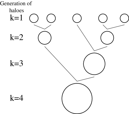
Figure 1: Example of generation and merging history of haloes. The first generation haloes include no progenitors. The final halo belongs to the fourth generation, and is formed by the merger of the third generation halo and the second generation halo. We omit the accreting matter in this figure.

Now we define the generation of haloes as follows (see Fig.1). A collapsed block which has no progenitors is defined as a first generation halo $(k=1)$. The $k$-th generation halo is defined as a halo which includes the $(k-1)$-th generation pre-existing haloes whose number specifying their generations is the largest of its progenitors. If the new halo is a $k$-th generation halo ($k\geq 2$), these three components of angular momentum are expressed as

$${\bf L}_{spin} \equiv \sum_{i}{\bf L}_{spin,i}^{k^{\prime}(i)}~{}~{}~{}[1\leq k^{\prime}(i)\leq k-1],$$ (11)

$${\bf L}_{orb} \equiv \sum_{i}M_{i}({\bf q}_{i}-{\bf q}_{CM})\times({\bf v}_{i}-{\bf v}_{CM})\left(\frac{1.05}{\delta^{k}}\right)^{\frac{3}{2}},$$ (12)

$${\bf L}_{acc} \equiv M_{cell}\sum_{j}({\bf q}_{j}-{\bf q}_{CM})\times({\bf v}_{j}-{\bf v}_{CM})\left(\frac{1.05}{\delta^{k}}\right)^{\frac{3}{2}},$$ (13)

where the subscripts $i$ and $j$ stand for the isolated pre-existing haloes just before the new common halo collapses and cells of accreting matter respectively, so that ${\bf L}_{spin,i}^{k^{\prime}(i)},M_{i},{\bf q}_{i}$ and ${\bf v}_{i}$ are respectively the spin, mass, position and velocity of the centre-of-mass of the $i$-th progenitor. The superscripts $k$ and $k^{\prime}(i)$ show the generation of haloes. The isolated $k^{\prime}(i)$-th generation pre-existing haloes $[k^{\prime}(i)\geq 1]$ merge together into the $k$-th generation halo. The subscript $CM$ denotes the centre-of-mass of the new halo, $M_{cell}$ is a mass of one cell, and $\delta^{k}$ is associated with a new collapsed $k$-th generation halo, because the angular momenta of the orbital and accreting matter grow until the maximum expansion time of the new collapsed halo. Finally, we obtain a total angular momentum ${\bf L}_{spin}^{k}$ of the new collapsed halo by summing the above quantities,

$${\bf L}_{spin}^{k}={\bf L}_{spin}+{\bf L}_{orb}+{\bf L}_{acc}.$$ (14)

If this new collapsed $k$-th generation halo will merge again into a collapsed halo at a later epoch, ${\bf L}_{spin}^{k}$ is used as ${\bf L}_{spin,i}^{k}$ in the estimation of the angular momentum ${\bf L}^{k+1}$ of the later collapsed $(k+1)$-th generation halo. Note that when a first ($k=1$) generation halo collapses, this halo has no progenitors, so this halo is formed by only the accreting matter. Therefore the angular momentum of this halo is estimated by only eq.(13), i.e., ${\bf L}_{spin}^{1}={\bf L}_{acc}$. This estimation is the same as in the homogeneous collapse, eq.(2).

When considering a homogeneous case as in the previous analytical work (Heavens & Peacock 1988; Catelan & Theuns 1996a, b), we first calculate the regions of collapsed haloes as described in Section 3. Then we average the density contrasts of cells in each halo, and obtain the averaged density contrast $\delta_{avg}$. Finally, using only eq.(13), we obtain the angular momentum of each halo. In this equation, $\delta^{k}$ corresponds to the above averaged density contrast $\delta_{avg}$.

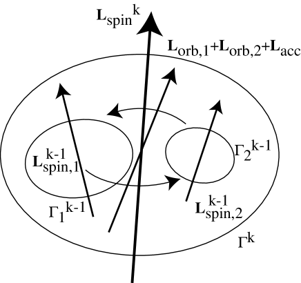
Figure 2: Schematic description of dark halo formation including two pre-existing haloes. The halo labelled by the superscript $k$, which is surrounded by the ellipsoid $\Gamma^{k}$, is formed through the merger of the two progenitors labelled by $k-1$, which are surrounded by the ellipsoids $\Gamma_{1}^{k-1}$ and $\Gamma_{2}^{k-1}$, and the accretion of matter within $\Gamma^{k}$. These two progenitors have their spins ${\bf L}_{spin,1}^{k-1}$ and ${\bf L}_{spin,2}^{k-1}$, and their orbital angular momenta around the centre-of-mass of the new common $k$-th generation halo ${\bf L}_{orb,1}$ and ${\bf L}_{orb,2}$. These orbital angular momenta and the accreting matter’s angular momentum ${\bf L}_{acc}$ grow until the maximum expansion time of the new common halo. Thus the angular momentum of the new common halo is obtained by ${\bf L}_{spin}^{k}={\bf L}_{spin}+{\bf L}_{orb}+{\bf L}_{acc}$.

In Fig.2, we show the schematic description of dark halo formation including two progenitors. In this case, two $(k-1)$-th generation progenitors merge together into a new $k$-th generation larger halo with accreting matter. So the spin component of the new $k$-th generation halo is obtained as ${\bf L}_{spin}={\bf L}_{spin,1}^{k-1}+{\bf L}_{spin,2}^{k-1}$, and the total angular momentum, namely, the spin of the new $k$-th generation halo is ${\bf L}_{spin}^{k}={\bf L}_{spin}+{\bf L}_{orb}+{\bf L}_{acc}$.

5 RESULTS

In this section we show final distributions of the spin angular momentum $|{\bf L}|$ and the mass-weighted angular momentum $|{\bf L}|/M^{5/3}$, which are similar to those used by Heavens & Peacock (1988) and Catelan & Theuns (1996a). We assume that linear density fluctuations obey a random Gaussian distribution with a power-law power spectrum $P(k)\propto k^{n}$, where $n=0$ and $-2$. We consider only the Einstein-de Sitter background universe ($\Omega=1,\Lambda=0$). The calculating box size is $L_{\mbox{box}}=128$. The normalization of the power spectrum is such that the variance of the density contrasts equals unity at a block with eight cells. The overlapping parameters are set as $x=y=1/2$, and $x=1/8$ and $y=1/2$.

The number of haloes finally obtained is about $1.6\times 10^{4}$ for $n=0$ and about $9\times 10^{3}$ for $n=-2$ in one calculating box. The following results are averaged over five realizations, therefore our investigations are statistically robust.

In all figures, the displayed values of the mass, the angular momentum and the time are normalised. The time $t$ is normalized by the present time $t_{0}$. Physical values for the mass and the angular momentum at the present epoch may be obtained through $M_{phys}=m_{*}M$ and ${\bf L}_{phys}=m_{*}l_{*}{\bf L}$, where $m_{*}=1.4\times 10^{14}M_{\odot}$ and $l_{*}=3\times 10^{6}\mbox{km~{}s${}^{-1}$~{}kpc}$ for the Hubble parameter $h=0.5$, which is normalised by 100 km s^-1Mpc^-1 ($m_{*}$ corresponds to the mass of one cell and $l_{*}$ is determined by the resolution of the calculation). Note that these physical values are scaled as $m_{*}(z)=m_{*}(1+z)^{-6/(3+n)}$ because of the scale-free power spectrum. For example, $m_{*}\simeq 3\times 10^{9}M_{\odot}$ at $z=5$ in the case of $n=-2$.

In the following, we consider three cases in which to estimate the angular momentum. One is the merger case, in which ${\bf L}$ is given by eq.(14). Second is the non-orbital case, in which we remove the component of orbital angular momentum, ${{\bf L}}_{orb}$. Third is the homogeneous case. In the homogeneous case, we estimate a region occupied by each halo, then we average the density contrasts in the region; after that, we estimate the maximum expansion time via the averaged density contrast by using eq.(10). Thus each cell which belongs to a halo has the same maximum expansion time, that is, the halo is treated as a homogeneous density object in the homogeneous case. By using this maximum expansion time, we obtain the angular momentum of the final halo through the velocity field, as in eq.(13). This procedure is almost the same as that in the previous work (Heavens & Peacock 1988; Catelan & Theuns 1996a, b).

In all cases, we consider only haloes with mass larger than nine cells, because of the numerical resolution. Also, we consider only final haloes with an averaged density contrast larger than 1.69 in the homogeneous case, because each collapsing block must satisfy the criterion of the spherical collapse.

Figure 3: Mass dependence of mean angular momentum in the case of $x=1/2$. upper panel: n=0, lower panel: n=-2. The dashed lines show the homogeneous case (HOM). The solid lines show the merger case (MRG). The dotted lines show those without orbital angular momentum (the non-orbital case; NOR). The thick solid lines show the lines proportional to $L\propto M^{5/3}$.

Figure 4: The same as Fig.3 but for $x=1/8$. upper panel: n=0, lower panel: n=-2.

5.1 Mass dependence of angular momentum

First, we show the mean angular momentum against the mass of the haloes in the case of $x=1/2$ (Fig.3) and $x=1/8$ (Fig.4). The horizontal axis denotes the mass, that is, the number of cells of each halo. The vertical axis denotes angular momentum averaged over each mass bin. The solid lines correspond to the merger case. The dotted lines and dashed lines correspond to the non-orbital case and the homogeneous case, respectively. The short thick solid lines denote $L\propto M^{5/3}$. The minimum mass in the figures corresponds to a halo with eight cells ($\log{8}\sim 0.9$), and the values of the mean angular momentum in the minimum mass are unphysically small because of the numerical resolution. In the homogeneous case, there are no data for larger-mass because the averaged density contrasts in large haloes are smaller than 1.69.

The deviation from the thick line $L\propto M^{5/3}$ probably results from the boundary effect of objects, caused by the artificial blocks and cells. We will show this boundary effect in a future work.

In the case of $x=1/2$ (Fig.3), the differences among the lines are rather small, but we find tendencies: the angular momentum in the merger case is smaller than in the homogeneous case, and the angular momentum decreases slightly when the orbital angular momentum component is removed. We find that orbital angular momentum does not play an important role in the case of $x=1/2$. In the case of $x=1/2$, haloes grow almost solely through accretion events; large blocks with $8^{3}$ or more cells should collapse in order to merge two or more pre-existing haloes. However, the probability that such large blocks would collapse, including two or more haloes and satisfying the criterion (c), is small. Thus merger events between two or more pre-existing haloes occur rarely. This is the reason why orbital angular momentum does not play an important role in the case of $x=1/2$.

On the other hand, when $x=1/8$ we can see that the difference between the merger case and the non-orbital case is large, about one order of magnitude at $\log M\sim 3.5$, while the difference between the merger case and the homogeneous case is not pronounced (Fig.4). Under these conditions, the merger events occur easily. Since the orbital angular momentum can grow until a relatively later time, the role of the orbital angular momentum becomes important.

In both cases, we find that the mass dependence of the homogeneous case is almost the same as that of the merger case, while the contribution of the orbital angular momentum to the total angular momentum depends on the overlapping parameter $x$. These properties are almost independent of the spectral index $n$. It seems to be strange that the merger and the homogeneous cases lead to the same results independently of the value of $x$. We will investigate this problem by considering the angular momentum distribution in detail in the next subsection.

5.2 Angular momentum distributions

To investigate the angular momentum distribution in detail, let us consider the distributions of the angular momentum $L$ in Fig.5a ($x=1/2$) and in Fig.6a ($x=1/8$), and the mass-weighted angular momentum $L/M^{5/3}$ in Fig.5b ($x=1/2$) and in Fig.6b ($x=1/8$). Each figure includes the merger case and the homogeneous case. The solid lines show the distributions for the merger case, and the dashed lines the homogeneous case. The thick lines correspond to the spectral index $n=0$, and the thin lines mark $n=-2$.

In the case of $x=1/2$, we can see that the distributions for the homogeneous case are almost the same as those of the merger case. The degree of the difference between them is the same order of magnitude as the difference between the mean values shown in Fig.3. This result suggests that the final distribution of the angular momentum does not change very much when considering the merger effect.

For $x=1/8$, it seems that the distributions of $L$ in the merger case become wider especially in the case of $n=-2$ (Fig.6a). It should be noted that haloes with averaged density contrast smaller than 1.69 are removed in the homogeneous case, so the difference between the homogeneous and the merger cases is apparently large at higher angular momentum. In Fig.6b, we do not need to take care of this removal effect in the homogeneous case, because the mean angular momentum is nearly proportional to $M^{5/3}$ (see the thick solid line in Fig.4). The distribution for the homogeneous case is also almost the same as that for the merger case when $x=1/8$. We find that the merger effect does not affect the final angular momentum distribution, independently of $x$.

Still, the difference between the merger case and the homogeneous case is very small. This fact is considered below in more detail.

Figure 5: (a) Angular momentum distributions in the case of $x=1/2$. The thick lines denote the case of n=0, and the thin lines n=-2. The solid lines denote the merger case, and the dashed lines homogeneous case. (b) Mass-weighted angular momentum ($L/M^{5/3}$) distributions in the case of $x=1/2$. Types of the lines are the same as (a).

Figure 6: The same as Fig.5, but for $x=1/8$.

5.3 Distributions of maximum expansion time

In this subsection, first we investigate the distribution of a product of mass and the maximum expansion time of each halo, because the absolute value of angular momentum depends strongly on the maximum expansion time. This quantity is represented as

$$M\langle t_{m}\rangle \equiv \sum_{i}M_{cell}t_{m,i},$$ (15)

where $t_{m,i}$ is the first maximum expansion time of the cell labelled by $i$, which is defined below in each model. The sum is carried out in the region of each halo. So the angle brackets mean the average in the region of each halo. We distinguish the merger case from the homogeneous case by superscripts ‘MRG’ and ‘HOM’, e.g., $\langle t_{m}^{MRG}\rangle$ and $\langle t_{m}^{HOM}\rangle$, because values of $t_{m,i}$ are different in the case of the merger and the homogeneous cases. In the homogeneous case $t_{m,i}^{HOM}$ of a cell is estimated from the density contrast averaged over the region of each halo, therefore cells which belong to the same final halo have the same maximum expansion time. However, in the merger case $t_{m,i}^{MRG}$ is estimated from the density contrast of a block to which the cell belongs.

We show the distributions of $M\langle t_{m}\rangle$ in Fig.7a ($x=1/2$) and in Fig.8a ($x=1/8$), and $\langle t_{m}\rangle/M^{2/3}$ in Fig.7b ($x=1/2$) and in Fig.7b ($x=1/8$), in the merger and the homogeneous cases, respectively, because the dependences on the maximum expansion time $L$ and $L/M^{5/3}$ in Figs.5 and 6 are the same as $M\langle t_{m}\rangle$ and $\langle t_{m}\rangle/M^{2/3}$. The solid lines show the distributions for the merger case, and the dashed lines represent the homogeneous case. The thick lines and the thin lines mark the spectral index $n=0$ and $n=-2$, respectively.

In the case of $x=1/2$, the differences between the merger case and the homogeneous case are about 0.3 order of magnitude at $\log(M\langle t_{m}\rangle)\sim 1-2$ (Fig.7a) and at the range of $\log(M\langle t_{m}\rangle)\sim-2.5--1.5)$ (Fig.7b). These differences are large as compared with the distribution of the angular momentum shown in Fig.5. This is caused by the numerous cells which halt the growth of the angular momentum earlier in the merger case than in the homogeneous case, especially for large haloes. The result in the case of $x=1/8$ is the same as for $x=1/2$. Therefore, we must explain the reason why the distribution of the angular momentum is not changed much by the merger effect, as compared to the distribution of the maximum expansion time.

Figure 7: Distributions of product of mass $M$ and maximum expansion time $\langle t_{m}\rangle$ in the case of $x=1/2$. (a) distributions of $M\langle t_{m}\rangle$. (b) $\langle t_{m}\rangle/M^{2/3}$. The solid lines show the distributions for the merger case. The dashed lines show those for the homogeneous case.

Figure 8: The same as Fig.7 but for $x=1/8$.

We should consider the effect of the direction of the angular momentum. If the growth of the angular momenta of the proto-objects with a direction close to the direction of the final angular momentum halts later than the growth of the angular momenta of the other proto-objects with an opposite direction, in a region which becomes a present-time halo, the total angular momentum of the halo can become larger in spite of the averaged maximum expansion time $\langle t_{m}^{MRG}\rangle$ being small. Thus we investigate the maximum expansion time, weighted by the direction (which will be defined below).

Defining the time-independent vector part of the angular momentum of a cell labelled by $i$ as

$${\bf L}^{vec}_{i}=M_{cell}({\bf q}_{i}-{\bf q}_{CM})\times({\bf v}_{i}-{\bf v}_{CM}),$$ (16)

the absolute values of the angular momentum for the merger case and for the homogeneous case are as follows

$$|{\bf L}^{MRG}| = \left|\sum_{i}{\bf L}^{vec}_{i}t_{m,i}^{MRG}\right|,$$ (17)

$$|{\bf L}^{HOM}| = \left|\sum_{i}{\bf L}^{vec}_{i}\right|\frac{\sum_{i}M_{cell}t_{m,i}^{HOM}}{M}=\left|\sum_{i}{\bf L}^{vec}_{i}\right|\langle t_{m}^{HOM}\rangle,$$ (18)

respectively. Considering the merger case, defining $\theta_{f}$ as the angle of the direction of the final angular momentum, we can transform eqs. (17) and (18) into

$$|{\bf L}^{MRG}|=\sum_{i}|{\bf L}^{vec}_{i}|\cos(\theta_{i}-\theta_{f})t_{m,i}^{MRG},$$ (19)

$$|{\bf L}^{HOM}|\simeq\sum_{i}|{\bf L}^{vec}_{i}|\cos(\theta_{i}-\theta_{f})\langle t_{m}^{HOM}\rangle.$$ (20)

So we investigate the direction-weighted maximum expansion time instead of $\langle t_{m}\rangle$,

$$\langle t_{m}\rangle_{\cos\theta}\equiv\frac{\sum_{i}\cos(\theta_{i}-\theta_{f})t_{m,i}^{MRG}}{\sum_{i}\cos(\theta_{i}-\theta_{f})}.$$ (21)

Then

$$|{\bf L}^{MRG}|\simeq\sum_{i}|{\bf L}_{i}^{vec}|\cos(\theta_{i}-\theta_{f})\langle t_{m}\rangle_{\cos\theta}.$$ (22)

Here we have used the assumption that the absolute value of ${\bf L}_{i}^{vec}$ is statistically independent of the direction of ${\bf L}_{i}^{vec}$. Thus if $\langle t_{m}^{HOM}\rangle\sim\langle t_{m}\rangle_{\cos\theta}$ it is expected that $|{\bf L}^{HOM}|\simeq|{\bf L}^{MRG}|$.

We show the relation of the direction-weighted maximum expansion time $\langle t_{m}\rangle_{\cos\theta}$, the non-weighted maximum expansion time $\langle t_{m}^{MRG}\rangle$, and the averaged maximum expansion time $\langle t_{m}^{HOM}\rangle$ in Fig.9 ($x=1/2$) and in Fig.10 ($x=1/8$). Each dot corresponds to a halo. The left panels show results for the spectral index $n=0$ and the right panels for $n=-2$. We show the comparisons of $\langle t_{m}^{HOM}\rangle$ with $\langle t_{m}\rangle_{\cos\theta}$ in the upper panels, and with $\langle t_{m}^{MRG}\rangle$ in the lower panels. The solid straight lines have a unity slope.

The difference of the extents of the distributions of dots in the horizontal axis between the case of $n=0$ and $n=-2$ is a result of the difference of the power spectrum of density fluctuation field. The mass dependence of the maximum expansion time is

$$t_{m}\propto a_{M}^{3/2}=\left(\frac{1.05}{\delta}\right)^{3/2}\sim M^{\frac{3+n}{4}},$$ (23)

thus the distribution of dots in the case of $n=0$ spread out wider than those in $n=-2$.

In the lower panels, there are most of dots below the solid lines, as we have already found in Figs.7 and 8. However, in the upper panels, the dots are distributed in a wider range in the vertical axis than those in the lower panels. This result shows that in some merging histories, the growth of angular momentum with the opposite direction to the final one happens to halt earlier than that with the same direction of the final one, and so some haloes satisfy the condition $\langle t_{m}\rangle_{\cos\theta}\geq\langle t_{m}^{MRG}\rangle$. Then $\langle t_{m}\rangle_{\cos\theta}\sim\langle t_{m}^{HOM}\rangle$ while the dispersion of $\langle t_{m}\rangle_{\cos\theta}$ is large.

This is the main reason why the distribution of the angular momentum in the merger case is almost the same as that in the homogeneous case. Although $\langle t_{m}^{MRG}\rangle$ is smaller than $\langle t_{m}^{HOM}\rangle$, proto-objects having an angular momentum with the same direction as the final one have a larger maximum expansion time $t_{m,i}^{MRG}$, and those with the opposite direction have smaller maximum expansion time. So the final angular momentum becomes almost the same as that for the homogeneous case. Therefore both distributions are very much alike.

Figure 9: Distributions of maximum expansion time $\langle t_{m}\rangle$ in the case of $x=1/2$. The solid lines denote those with a unity slope. (a) Distributions of $\langle t_{m}^{HOM}\rangle$ (the homogeneous case) v.s. $\langle t_{m}\rangle_{\cos\theta}$ in the case of $n=0$. (b) Distributions of $\langle t_{m}^{HOM}\rangle$ (the homogeneous case) v.s. $\langle t_{m}^{MRG}\rangle$ (the merger case) in the case of $n=0$. (c) The same as (a), but for $n=-2$. (d) The same as (b), but for $n=-2$.

Figure 10: The same as Fig.9 but for $x=1/8$.

5.4 Orbital angular momentum

In order to investigate the contribution of the orbital angular momentum to the total angular momentum, in Fig.11 we show the case in which we remove the component of the orbital angular momentum (the non-orbital case) in the case of $x=1/2$. The solid lines show the total angular momentum (${\bf L}_{spin}+{\bf L}_{acc}+{\bf L}_{orb}$) in Fig.11a and those divided by $M^{5/3}$ in Fig.11b for the merger case, and the dashed lines show the total angular momentum without the orbital angular momentum component, that is, ${\bf L}_{spin}+{\bf L}_{acc}$ in Fig.11a and those divided by $M^{5/3}$ in Fig.11b. The thick lines denote the spectral index $n=0$, and the thin lines $n=-2$. In the case of $x=1/2$, reflecting the small differences in Fig.3, the differences between the merger case and the non-orbital case are very small. As already mentioned in Section 5.1, in the case of $x=1/2$, haloes grow almost solely through the accretion events, and the merger events between two or more pre-existing haloes occur rarely. Thus the contribution of the orbital angular momentum is small.

In Fig.12, we show the same results as in Fig.11 but for the case of $x=1/8$. In the upper panel, in contrast to Fig.11a, the differences at higher angular momentum are larger than those at lower angular momentum. In the case of $x=1/8$, two or more pre-existing haloes can merge with each other many times. We find that the number of occurrences of the merger event is nearly proportional to $0.01M^{1.25}$ in the case of $n=0$ and $0.02M$ in the case of $n=-2$ for larger haloes than $\sim 100$ cells. Then haloes with a larger mass generally experience many merging events. Moreover, the haloes with larger mass have larger angular momentum. Hence the contribution of the orbital angular momentum of a halo is greater for the halo with a larger total angular momentum.

Figure 11: (a) Angular momentum distributions in the case of $x=1/2$. The thick lines denote the case of $n=0$, and the thin lines $n=-2$. The solid lines are the same as Fig.5 (the merger case), and the dashed lines denote the non-orbital case (angular momentum without the orbital angular momentum). (b) Mass-weighted angular momentum $(L/M^{5/3})$ distributions in the case of $x=1/2$. Types of the lines are the same as (a).

Figure 12: The same as Fig.11 but for $x=1/8$.

5.5 Spin parameter $\lambda$

In this subsection, we show the distributions of the dimensionless spin parameter $\lambda$, which is defined as

$$\lambda\equiv\frac{L|E|^{1/2}}{GM^{5/2}},$$ (24)

where $E$ is the total energy of a halo with mass $M$ and angular momentum $L$. We estimate $E$ by summing kinetic energies and gravitational energies of cells within each halo.

This spin parameter corresponds to the ratio of the rotational kinetic energy to the gravitational energy, so an object with $\lambda\sim 1$ is fully rotationally supported. It has been reported that typically $\lambda\approx 0.08$ for the theoretical predictions and for the N-body simulations, and $\lambda\sim 0.5$ for spirals and $\lambda\sim 0.05$ for ellipticals by observations. We need to know dissipational gas collapse process in order to compare the spin parameters obtained theoretically with those obtained by observations, but it is beyond the scope in this paper.

In Fig.13, we show the distributions of $\lambda$ in the merger (solid lines), homogeneous (dashed lines), and non-orbital cases (dotted lines) when $x=1/2$. Similarly, in Fig.14, we show the same lines as Fig.13 in $x=1/8$. In both cases, the values of $\lambda$ at the peaks of distributions in the merger case are lower than those in the homogeneous case, and are higher than those in the non-orbital case. These tendencies are the same as the results in the previous subsections. The rms values of $\lambda$ are $\sqrt{\langle\lambda^{2}\rangle}\simeq 0.07$ in the case of $n=0$ and $0.25$ in the case of $n=-2$ in the merger case. These are almost consistent with the previous theoretical predictions.

Figure 13: $\lambda$ distributions in the case of $x=1/2$. (a) $n=0$. (b) $n=-2$. The solid lines are the merger case, the dashed dashed lines denote the homogeneous case, and the dotted lines show the non-orbital case.

Figure 14: The same as Fig.13 but for $x=1/8$.

6 CONCLUSIONS AND DISCUSSION

In this paper we have analysed the acquisition and distribution of the angular momentum of proto-objects with inhomogeneous density distribution by using the merging cell model. The assumptions in our calculations are as follows: spherically symmetric collapse of each block, the overlapping criteria (see Section 3), and the growth of angular momentum proportional to the cosmic time $t$. We also assume that the halting time of the acquisition of angular momentum is determined by the maximum expansion time.

In almost all of the previous work, it has been suggested that proto-objects are homogeneous density ellipsoids, and that the maximum expansion time may be estimated from the smoothed density contrast. However, if we consider the hierarchical clustering scenarios on which most of the previous analyses of the angular momentum are based, we should consider the merger effect. In the hierarchical clustering scenario, it is natural that each proto-object has a different halting time in the acquisition of the angular momentum. Hence it is very important to consider the merging histories of dark haloes. However, we find no significant differences between the distributions of angular momentum for the merger and the homogeneous cases in our analyses by using the merging cell model. We find the reason for this by dividing the angular momentum into two components, that is, the time-independent vector and the maximum expansion time (see Section 5.3). The distribution of the maximum expansion time, which is directly influenced by the merging history, moves to the lower value. However, the angular momentum components that have a direction which is the same as that of the final angular momentum grow later than those with other directions. This is shown by comparing simply averaged maximum expansion time in each halo $\langle t_{m}^{MRG}\rangle$ with the direction-weighted maximum expansion time $\langle t_{m}\rangle_{\cos\theta}$. We find that many haloes satisfy $\langle t_{m}\rangle_{\cos\theta}\geq\langle t_{m}^{MRG}\rangle$. Thus, as these two effects cancel each other out, the difference between the merger case and the homogeneous case becomes negligible. Note that this conclusion is independent of the overlapping parameter $x$.

In our calculations, we use the scale-free power spectra, $P(k)\propto k^{n}$, where $n=0$ and $n=-2$. When we normalize $P(k)$ at the present epoch, the mass-scale in our investigation corresponds to the clusters of galaxies. However, we can scale the normalization to a galactic scale at high redshift because of the scale-free spectra (see Section 5). When we consider the galaxy formation processes, it may be important to analyse the process of the acquisition of the angular momentum of dark haloes at high redshift corresponding to the galaxy formation epoch, because the spins of dark haloes convert to those of the baryonic component, namely, galaxies at high redshift.

We also show the contributions of the orbital angular momentum of pre-exiting haloes when mergers occur. This analysis is enabled by using the semi-analytical models like the merging cell model. The difference between the merger case and the non-orbital case, which does not include the orbital angular momentum component strongly depends on the overlapping parameter $x$. In the case of $x=1/2$, in which there are not too many merger events between two or more pre-existing haloes, the contribution of the orbital angular momentum to the total angular momentum is small. On the other hand, in the case of $x=1/8$, the orbital angular momentum plays an important role. The contribution of the orbital angular momentum is about one order of magnitude larger than the contributions of the other components, which are the spin angular momentum and the angular momentum of the accreting matter. Note that it is easy for blocks to collapse in this case of $x=1/8$ and that there are many merger events. We cannot decide the value of the overlapping parameter $x$ without a detailed study of the overlapping condition, so we can only mention our conclusions qualitatively. However, even under this limitation, we find that the orbital angular momentum plays a significant role in the total angular momentum if merger events occur many times. When the evolution of the angular momentum of the baryonic component is considered, the process of the merging of galaxies as gaseous and stellar components will involve a release of angular momentum to dark matter and running away gas. So the distribution of the angular momentum of the gaseous component may follow the distribution without the orbital angular momentum. If elliptical galaxies are formed through such a merger process, and if spiral galaxies are formed without a loss of angular momentum of accreting gas, this result is very suggestive, because the observational difference between the angular momentum of ellipticals and spirals is also about one order of magnitude (see e.g. Fall 1983 or Fig.9 in Catelan & Theuns 1996a). Such tendencies are presented in Fig.4. We need hydro-dynamical simulations in order to decide whether the distribution of the angular momentum of galaxies is followed by the distribution that includes orbital angular momentum or not, since our model considers only dark matter component. One such baryonic effects has been discussed as the ‘angular momentum catastrophe’ in Weil, Eke & Efstathiou (1998).

As mentioned above, we assume the spherically symmetric collapse of each block in the merging cell model. For this reason, we need the overlapping parameter $x$. So we believe that we need a new model which includes nonspherical collapse in order to discuss the merger effect quantitatively. This study is in progress.

References

- [1] Barnes J., Efstathiou G., 1987, ApJ, 319, 575
- [2] Bardeen J.M., Bond J.R., Kaiser N., Szalay A.S., 1986, ApJ, 304, 15
- [3] Bower R.J., 1991, MNRAS, 248, 332
- [4] Caimmi R., 1989, A&A, 223, 29
- [5] Catelan P., Theuns, T., 1996a, MNRAS, 282, 436
- [6] Catelan P., Theuns, T., 1996b, MNRAS, 282, 455
- [7] Catelan P., Theuns, T., 1997, MNRAS, 292,225
- [8] Cole S., Kaiser N., 1988, MNRAS, 233, 637
- [9] Dalcanton J.J., Spergel D.N., Summers F.J., 1997, ApJ, 482, 659
- [10] Doroshkevich, A.G., 1970, Astrofizika, 6, 581
- [11] Efstathiou G. & Jones B.J.T., 1979, MNRAS, 186, 133
- [12] Eisenstein D.J., Loeb A., 1995, ApJ, 439, 520 (1995a)
- [13] Eisenstein D.J., Loeb A., 1995, ApJ, 443, 11 (1995b)
- [14] Fall S.M., 1983, in Athanassoula E., et., Internal Kinematics and Dynamics of Galaxies. IAU Symp. 100, Reidel, Dordrecht, p.391
- [15] Heavens A., Peacock J., 1988, MNRAS, 232, 339
- [16] Hoyle F., 1949, In Problems of Cosmological Aerodynamics, eds. Burgers J.M. & van de Hulst H.C. (Central Air Documents Office, Dayton)
- [17] Hoffman Y., 1986, ApJ, 301, 65
- [18] Hoffman Y., 1988, ApJ, 329, 8
- [19] Jimenez R., Heavens A.F., Hawkins M.R.S., Padoan P., 1997, MNRAS, 292, L5
- [20] Kauffmann G., White S.D.M., 1993, MNRAS, 261, 921
- [21] Lemson G., Kauffmann G., 1997, preprint, astro-ph/9710125
- [22] Mo H.J., Mao S., White S.D.M., 1998, MNRAS, 295, 319
- [23] Nagashima M., Gouda N., 1997, MNRAS, 287, 515
- [24] Peacock J.A., Heavens A.F., 1985, MNRAS, 217, 805
- [25] Peebles P.J.E., 1969, ApJ, 155, 393
- [26] Peebles P.J.E., 1993, The Principles of Physical Cosmology, Princeton: Princeton Univ. Press
- [27] Press W.H., Schechter P., 1974, ApJ, 187, 425
- [28] Quinn T., Binney J., 1992, MNRAS, 255, 729
- [29] Rodrigues D.D.C., Thomas P.A., 1996, MNRAS, 282, 631
- [30] Roukema B.F., Peterson B.A., Quinn P.J., Rocca-Volmerange B., 1997, MNRAS, 292, 835
- [31] Ryden B.S., 1988, ApJ, 329, 589
- [32] Ryden B.S., Gunn J.E., 1987, ApJ, 318, 15
- [33] Susa H., Sasaki M., Tanaka T., 1994, PTP, 92, 961
- [34] Warren M.S., Quinn P.J., Salmon J.K. & Zurek W.H., 1992, ApJ, 399, 405
- [35] Weil M.L., Eke V.R., Efstathiou G., 1998, preprint, astro-ph/9802311
- [36] White S.D.M., 1984, ApJ, 286, 38
- [37] Yano T., Nagashima M., Gouda N., 1996, ApJ, 466, 1
- [38] Zel’dovich Ya.B., 1970, A&A, 5, 84