How to Plant a Merger Tree

Abstract

We investigate several approaches for constructing Monte Carlo realizations of the merging history of virialized dark matter halos (“merger trees”) using the extended Press-Schechter formalism. We describe several unsuccessful methods in order to illustrate some of the difficult aspects of this problem. We develop a practical method that leads to the reconstruction of the mean quantities that can be derived from the Press-Schechter model. This method is convenient, computationally efficient, and works for any power spectrum or background cosmology. In addition, we investigate statistics that describe the distribution of the number of progenitors and their masses as a function of redshift.

1 Introduction

In the standard picture of modern structure formation, small-amplitude Gaussian density fluctuations, which perhaps arose from quantum fluctuations and were amplified by a period of rapid inflation, become more overdense with respect to their surroundings as the universe expands. Eventually the self-gravity acting on these regions becomes larger than the pressure of the expansion, and they collapse to form bound, virialized structures. In hierarchical models, such as the cold dark matter (CDM) family of models, the amplitude of the fluctuations decreases with increasing scale. Thus small mass objects form first, and are then incorporated into larger structures as time progresses. These dense, gravitationally bound structures provide the environments where galaxies can form. Hierarchical structure formation thus gives a natural explanation for the very complex observed large scale structure of the Universe, i.e. clusters, superclusters, filaments, etc.

One way to study this process is with N-body simulations. However, numerical simulations have familiar drawbacks. They are computationally expensive, so it is difficult or impossible to explore a wide range of models or different realizations of the same model. In addition memory and time limitations make it impossible to attain the mass and force resolution required to simultaneously study objects from dwarf galaxies ($\sim 10^{9}\mbox{$M_{\odot}$}$) to clusters ($\sim 10^{15}\mbox{$M_{\odot}$}$). Semi-analytic methods are therefore an important alternative.

The model developed by ?) provides a simple but relatively effective framework for the description of the mass history of particles in a hierarchical universe with Gaussian random phase initial perturbations. The focus of the original Press-Schechter model was the derivation of the multiplicity function of non-linear objects (“halos”) as a function of redshift, i.e. the “mass function” or number density of halos of a given mass at a redshift $z$. This prediction has been tested quite extensively and found to be in relatively good agreement with N-body simulations [Efstathiou et al. (1988), Gelb & Bertschinger (1994), Lacey & Cole (1994), Ma (1996), Gross et al. (1998)]. The Press-Schechter theory was extended to give the conditional probability that a particle in a halo of mass $M_{0}$ at $z_{0}$ was in a halo of mass $M_{1}$ at an earlier redshift $z_{1}$, leading to an expression for the conditional mass function [Bower (1991), Bond et al. (1991)]. The extended Press-Schechter formalism can also be manipulated to obtain expressions for halo survival times, formation times, and merger rates [Lacey & Cole (1993), hereafter LC93], which have also been shown to agree reasonably well with the results from N-body simulations [Lacey & Cole (1994)].

The computation of these mean quantities within the Press-Schechter model is straightforward. However, for certain purposes one would like to go beyond this. In particular, the semi-analytic approach to modeling galaxy formation (cf. [Kauffmann et al. (1993)], [Cole et al. (1994)]) attempts to describe the formation history of galaxies and gas within dark matter halos, including simplified hydrodynamics, star formation, supernova feedback, galaxy-galaxy merging, and stellar population synthesis. These models rely on the construction of a “merger tree”, which involves predicting the masses of progenitor halos and the redshifts at which they merge to form larger halos. Galaxies initially form in their own halo and are traced as they are incorporated into larger halos, and eventually perhaps merge with other galaxies. A halo of a given mass may have a variety of merging histories, and the properties of galaxies that form within this halo presumably depend to some extent on the details of this history.

Most of the previous work using semi-analytic models has focussed on reproducing or predicting mean quantities and qualitative trends. However, as observational data continues to improve, one would like to be able to investigate whether the broader properties of the predicted distribution of model galaxies are consistent with the observations. For example, there has already been some investigation of whether the scatter in the observed Tully-Fisher relation [Eisenstein & Loeb (1996)], and in the color-magnitude and line-strength velocity-dispersion (Mg-$\sigma$) relations [Kauffmann (1996)] in merger models is consistent with observations. Before we can trust the models for evaluating these kinds of questions, we must ensure that the merger trees not only satisfy the mean properties readily predicted by the extended Press-Schechter model, but ideally also the full distribution function. As we shall see, accomplishing this goal is far from straightforward and has not been thoroughly investigated in previous work on this subject.

In this paper, we discuss some of the practical and theoretical difficulties of using the extended Press-Schechter model to create Monte Carlo merger histories of dark matter halos. We mention some limitations of the previously proposed methods for the construction of merger trees, and the motivation for developing a new approach. We discuss several unsuccessful approaches, in an attempt to clarify some aspects of this problem as well as to prevent others from following the same dead ends. In addition, the formalism we present may be useful in future work on this subject, as the final approach that we present seems to be effective and convenient, but it is still not rigorous. A primary motivation for embarking on this project was to develop a method that reproduces the full joint probability distribution, rather than just the mean. Our method is not guaranteed to do so, and further investigation of this question requires a comparison with N-body simulations. This will be presented in a companion paper [Somerville et al. (1998)].

In §2, we give a brief introduction to the Press-Schechter formalism. In §3 we summarize some of the previous methods for creating merger trees. In §4, we describe the source of some difficulties one encounters in attempting to use the extended Press-Schechter formalism to construct merger trees. We develop a simple model of the joint probability distribution in §5, and attempt to use it to construct merger trees. In §6, we present a completely different approach which eventually leads to our successful method, described in §6.3. In §7, we investigate the distribution of progenitor number and mass given by our successful method. We summarize and conclude in §8.

Readers who are only interested in the successful method may skip to §6.

2 The Press-Schechter Formalism

The Press-Schechter model [Press & Schechter (1974)] is based on a combination of linear growth theory, spherical collapse theory, and the properties of Gaussian random fields. Suppose that we have smoothed the initial density distribution on a scale $R$ using some spherically symmetric window function $W_{M}(r)$, where $M(R)$ is the average mass contained within the window function. There are various possible choices for the form of the window function (cf. [Lacey & Cole (1993)]), and the relation between $M$ and $R$ will clearly depend on this choice. We use a real-space top hat window function, $W_{M}(r)=\Theta(R-r)(4\pi R^{3}/3)^{-1}$, where $\Theta$ is the Heaviside step function. In this case $M=4\pi\rho_{0}R^{3}/3$, where $\rho_{0}$ is the mean mass density of the universe. The mass variance $S(M)\equiv\sigma^{2}(M)$ may be calculated from

$$\sigma^{2}(M)=\frac{1}{2\pi^{2}}\int P(k)W^{2}(kR)k^{2}{\rm d}k\,,$$ (1)

where $P(k)$ is the mass power spectrum, and $W(kR)$ is the Fourier transform of the real space top-hat:

$$W(kR)=\frac{3[\sin(kR)-kR\cos(kR)]}{(kR)^{3}}.$$ (2)

The “excursion set” derivation due to ?) leads naturally to the extended Press-Schechter formalism that we will use extensively in this paper. The smoothed field $\delta(M)$ is a Gaussian random variable with zero mean and variance $S$. The value of $\delta$ executes a random walk as the smoothing scale is changed. Adopting an ansatz similar to that of the original Press-Schechter model, we associate the fraction of matter in collapsed objects in the mass interval $M,M+{\rm d}M$ at time $t$ with the fraction of trajectories that make their first upcrossing through the threshold $\omega\equiv\delta_{c}(t)$ in the interval $S,S+{\rm d}S$. This may be translated to a mass interval through equation (1). The halo multiplicity function (here in the notation of LC93) is then:

$$f(S,\omega){\rm d}S=\frac{1}{\sqrt{2\pi}}\frac{\omega}{S^{3/2}}\exp{\left[-\frac{\omega^{2}}{2S}\right]}{\rm d}S\,.$$ (3)

The conditional mass function, the fraction of the trajectories in halos with mass $M_{1}$ at $z_{1}$ that are in halos with mass $M_{0}$ at $z_{0}$ ($M_{1}<M_{0}$, $z_{0}<z_{1}$) is

$$f(S_{1},\omega_{1}\mid S_{0},\omega_{0}){\rm d}S_{1}=$$ (4)

$$\frac{1}{\sqrt{2\pi}}\frac{(\omega_{1}-\omega_{0})}{(S_{1}-S_{0})^{3/2}}\exp{\left[-\frac{(\omega_{1}-\omega_{0})^{2}}{2(S_{1}-S_{0})}\right]}{\rm d}S_{1}\,.$$

The probability that a halo of mass $M_{0}$ at redshift $z_{0}$ had a progenitor in the mass range $(M_{1},M_{1}+{\rm d}M_{1})$ is given by (LC93):

$$\frac{{\rm d}P}{{\rm d}M_{1}}(M_{1},z_{1}\mid M_{0},z_{0}){\rm d}M_{1}=$$ (5)

$$\frac{M_{0}}{M_{1}}f(S_{1},\omega_{1}\mid S_{0},\omega_{0})\left|\frac{{\rm d}S}{{\rm d}M}\right|{\rm d}M_{1}\,,$$

where the factor $M_{0}/M_{1}$ converts the counting from mass weighting to number weighting.

All of the results presented in this paper have been calculated for an $\Omega=1$ universe with $H_{0}=50\;\mbox{km s${}^{-1}$ Mpc${}^{-1}$}$. The power spectrum is obtained from the fitting formula of ?) with $\Gamma=0.21$ and $\sigma_{8}=0.6$. This is the $\tau$CDM model of ?), and has been chosen because the slope of the power spectrum on galaxy scales is consistent with observations. However, our results are equally valid for any assumed power spectrum or cosmology. The one exception that we know of is the case of a universe with a “hot” dark matter component, such as a massive neutrino (CHDM or MDM type models). The standard extended Press-Schechter formalism does not properly treat the evolution due to the changing free-streaming length of the neutrino in such models. All of the expressions given are valid for a general cosmology unless otherwise noted.

3 Previous Methods

The development of techniques for constructing Monte Carlo realizations of the merging history of dark matter halos [Kauffmann & White (1993), Cole & Kaiser (1988), Cole (1991), Lacey & Cole (1993)] using the extended Press-Schechter formalism has allowed a great deal of progress to be made in the use of semi-analytic methods for studying galaxy formation and evolution. ?) developed a method for constructing merger trees which addresses the problem of simultaneously reproducing the average number of halos given by Eqn. 5 and imposing the constraint that the mass of a halo be equal to the sum of the masses of its progenitors at every stage. To do this they impose a grid in mass and redshift. For the first step in redshift, they then create a list of halos, where the number of halos with mass $M_{i}$ is given by $N(M_{i})=N_{\rm ens}\>{\rm d}N/{\rm d}M(M_{i})\>\Delta M_{i}$, rounded to the nearest integer. $N_{\rm ens}$ is some large number of ensembles, typically $N_{\rm ens}\sim 100$. The progenitors are randomly assigned to ensembles, starting with the largest and working in order of decreasing mass. The probability of assignment is proportional to the amount of remaining free mass, with the constraint that the total mass of the progenitors cannot exceed the mass of the parent. This process is repeated for all the steps in the redshift grid.

This algorithm is guaranteed to exactly reproduce the mean number of halos of each mass at each redshift for the set of ensembles. However, it is possible to encounter a situation in which the next halo does not fit into any of the ensembles. In order to get around this problem, mass conservation is only enforced in an approximate way (G. Kauffmann, private communication). There are also some practical drawbacks to this method. It is necessary to generate a large number of ensembles and store them, which is somewhat inconvenient. An arbitrary grid in halo mass and redshift must be imposed. Also, because the function ${\rm d}N/{\rm d}M$ is very sharply peaked around $M_{0}$ for small $M_{0}$ or small redshift intervals $\Delta z$, the algorithm as described in ?) is sensitive to the binning used and is prone to numerical problems. The algorithm breaks down for certain choices of power spectrum. Finally, although the mean of the distribution is reproduced by construction, the partitioning of the halos into individual ensembles is ad-hoc and may or may not reproduce the higher moments of the distribution.

A different approach, referred to as the “Block model”, has been proposed by ?) and ?). A major drawback with this approach is that the halo masses always grow in discrete steps of factors of two. This is problematic for the purpose of semi-analytic galaxy formation modeling, in which one would like to follow individual galaxies with fairly fine time resolution. LC93 propose a generalization of the block model which removes this condition, but we show in Section 6.1 that this method produces halo mass distributions that are severely discrepant with the Press-Schechter model.

4 Difficulties of Trees

The first choice we must make if we want to construct a merger tree is whether to start from high redshift and merge together small clumps until the desired redshift is reached (as in an N-body simulation or, presumably, in the real universe), or, to start from the present day and work backwards in time, “disintegrating” the halos into their progenitors like a film run backwards. The extended Press-Schechter formalism provides expressions applicable to both situations. An important consideration is that we would like to eventually anchor our approach using the observed $z=0$ properties of galaxies, which are presumably the most secure. In addition, because we lack any information about spatial correlations, if we go forward in time, we do not know which small clumps to combine with which. It may be possible to get around this problem somehow, but for now we pursue the “disintegration” approach, in which we postulate the existence of a “parent” halo of a given mass $M_{0}$ at redshift $z_{0}$ and break it into its “progenitors” working backwards in time.

It might appear a simple matter to construct a merger tree by simply picking the masses of the progenitors of our parent halo at some earlier redshift $z_{1}$ from the expression for ${\rm d}P/{\rm d}M(M_{1},z_{1}|M_{0},z_{0})$ given by Eqn. 5 above, then repeating this process starting from each progenitor in turn for the next step back in time. Two difficulties immediately arise in implementing this approach. First, from inspection of Eqn. 5, the number of halos clearly diverges as the mass goes to zero. However, note that the mass contained in small halos (Eqn. 4) does not diverge as $M\rightarrow 0$. In order to pick masses from the number weighted probability function numerically, it is necessary to introduce a cutoff mass, or effective mass resolution, $M_{l}$.

The second problem is that the progenitor masses must simultaneously be drawn from the distribution ${\rm d}P/{\rm d}M(M)$ and add up to the mass of the parent, $M_{0}$. The problem is that ${\rm d}P/{\rm d}M$ is just the average number of halos that one can make out of the mass $M_{0}f(M)\,{\rm d}M$. What we really want is the joint probability function for the set of progenitors $\{M_{1},\cdots,M_{n}\}$, ${\rm d}P_{n}/{\rm d}M(\{M_{1},\cdots,M_{n}\},z_{1}\mid M_{0},z_{0})$ with any value of $n<M_{0}/M_{l}$ . An obvious problem with the use of the single halo probability rather than the joint probability is that there is no guarantee that we will not at some stage pick a progenitor that does not “fit” in the halo: i.e. $M>M_{0}-\sum_{i}M_{i}$ where $M_{i}$ are the masses of all the previously picked progenitors. In addition, since the expression $P(M)$ only gives the probability that there was a progenitor of mass $M$ at an earlier time, we do not know a priori how many progenitors were present at the redshift $z_{1}$.

Having noted these points, we can write down some basic requirements for our merger tree construction algorithm:

1. The procedure must account for the mass contained in halos below the mass resolution $M_{l}$, which we will refer to as the “accreted mass”. However the results must be independent of the value of $M_{l}$.

2. The procedure should treat all progenitors equally, independently of the sequence in which they are chosen.

3. The procedure must simultaneously reproduce the distribution of the number of progenitors and their masses while conserving mass.

4. The algorithm should be numerically robust and must be possible to implement in a computationally efficient and convenient way.

We now demonstrate some problems that arise in several seemingly straightforward approaches to building the trees. The bold solid line in Figure 2 shows the prediction of the extended Press-Schechter model for the quantity ${\rm d}N/{\rm d}M$, the number of progenitors with mass $M$ for a parent halo with $M_{0}=5\,M_{l}$ after a single step in redshift from $z_{0}=0$ to $z_{1}=0.2$ (also called the conditional mass function). This is the quantity that a successful merging tree method must reproduce. In this figure and hereafter unless otherwise noted, all masses are given in units of the mass resolution $M_{l}$. Here we have used $M_{l}=1.0\times 10^{10}\mbox{$M_{\odot}$}$, but the results are independent of this value.

Figure 2: The number of progenitors with mass $m_{p}$ (conditional mass function) for a single step in redshift ($z_{0}=0$ to $z_{1}=0.2$). The bold solid line is the prediction of the extended Press-Schechter theory (Eqn. 5). The histograms were obtained by picking masses from the distribution $P(M,z_{1}\mid M_{0},z_{0})$ until the parent mass $M_{0}$ was exhausted. The dotted histogram (a) shows the results using the Naïve Method with Cutoff, and the short-dashed histogram (b) shows the results of using the Naïve Method with Truncation (see text). The long-dashed histogram (c) uses Accretion Model Method 1, and the dot-dashed histogram (d) uses Accretion Model Method 2 (see text). All masses are in units of the minimum progenitor mass $M_{l}$.

In our first attempted method, the progenitor masses are chosen from Eqn. 5 until the mass reservoir $M_{0}$ is exhausted. The probability is set to zero for $M<M_{l}$. We have tried two ways of addressing the problem of mass “overflow” described above. One approach is to choose progenitors until the total mass exceeds $M_{0}$, and then to truncate the mass of the last progenitor. We will refer to this as the “Naïve Method with Truncation”. Another approach is to impose an upper mass cutoff, so that the probability is effectively set to zero for any values of $M$ that exceed the available mass. In effect we then choose the $i$-th progenitor from the modified distribution

$$P_{i}(M_{i})=P(M_{i})\Theta(M_{i}-M_{l})\Theta(M_{0}-\sum_{j=1}^{i}M_{j})\,,$$ (6)

where $P(M)$ is the original probability function from Eqn. 5 renormalized for its new range. No attempt is made to compensate for the contribution of masses below $M_{l}$. We refer to this as the “Naïve Method with Cutoff”. The results for the quantity ${\rm d}N/{\rm d}M$ (averaged over many ensembles) is shown by the histograms marked a (Cutoff) and b (Truncation) in Figure 2.

Both procedures clearly fail to correctly reproduce the conditional mass function predicted by the extended Press-Schechter model (Eqn. 5). Although the introduction of the upper mass cutoff to prevent choosing masses that are too large to fit in the current ensemble is somewhat more elegant than the brute force truncation, we see that it produces a shift towards smaller masses which leads to large excess of small mass halos. It should be noted that this figure shows only one step in redshift. The excess multiplies with each subsequent step in redshift, so that even a relatively small discrepancy quickly becomes very serious. It should also be noted that these problems are most pronounced when $M_{0}\approx M_{l}$ (as in the case shown in the figure). If $M_{0}\gg M_{l}$, the disagreement is not as bad.

5 The Accretion Model

We must introduce a self-consistent way of treating progenitors above and below the cutoff mass, $M_{l}$. It should be noted that although the contribution of masses $M<M_{l}$ may be negligible for halos with $M_{0}\gg M_{l}$, as the mass of the parent approaches the resolution limit it necessarily becomes a significant fraction of the total progenitor mass. Because every halo, regardless of its size, must be broken down into smaller and smaller pieces until all of the pieces fall below the mass resolution (this is what makes the process finite), the correct treatment of small halos is crucial for reconstructing the formation history of halos of all masses out to arbitrarily high redshift.

The basic idea behind this approach is never to treat any mass below $M_{l}$ in terms of progenitor number, but rather to find a complimentary description for it as accreted diffuse matter. We now introduce an arbitrary distinction in terminology to reflect this division. Let progenitors by definition have mass greater than the fixed mass resolution $M_{l}$. The aggregate contribution of all halos with $M<M_{l}$ will be referred to as accreted mass. A fully rigorous procedure should use the joint probability for progenitor number (not mass) above $M_{l}$, and accreted mass (not number of halos) below this mass scale.

We can now define a few more useful quantities. Given the mass of the parent halo $M_{0}$ and the redshift step $z_{0}\rightarrow z_{1}$, the average number of progenitors (recalling our definition above), is:

$$\bar{N}\equiv\langle N_{p}(M\,|M_{0})\rangle=\int_{M_{l}}^{M_{0}}\,{\rm d}M\,\frac{M_{0}}{M}\,P(M,z_{1}|M_{0},z_{0})\,.$$ (7)

We can also calculate the average fraction of $M_{0}$ that dwelt in the form of progenitor halos of mass $M>M_{l}$:

$$\bar{f}_{p}=\int_{M_{l}}^{\infty}{\rm d}M\,P(M,z_{1}|M_{0},z_{0})\,,$$ (8)

and the complimentary quantity for the average fraction of $M_{0}$ that came from “accreted” mass, $\bar{f}_{acc}=1-\bar{f}_{p}$.

Before we proceed, we would like to warn the reader that the contents of the remainder of this section are rather detailed and probably only of interest to the specialist. The formalism developed in the rest of this section is not used directly in the successful method that we will eventually derive. We urge the impatient reader to skip directly to §6.

From the above predictions we can try to evaluate what went wrong with our previous procedures (the “Naïve” methods). The predicted average number of progenitors for the case considered in Figure 2 ($M_{0}=5\,M_{l}$, $z_{0}=0$, $z_{1}=0.2$) is $\bar{N}=1.14$. The actual average number for one hundred Monte Carlo realizations using the Naïve Method with Truncation is $\bar{N}=2.1$, and for the Naïve Method with Cutoff it is $\bar{N}=2.3$. Thus we see that the mean of the distribution is shifted towards larger numbers of small mass halos. This motivates our goal in this section, which is to find the probability function ${\cal P}_{N}$ of having $N$ progenitors at redshift $z_{1}$ given the mass $M_{0}$ at a later redshift $z_{0}$, with the imposed cutoff of $M_{l}$.

Given $M_{0}$, $z_{0}$, and $z_{1}$, let $M_{1,p}$ be the mass of a progenitor, where by definition $M_{1,p}>M_{l}$. However, during the time interval $\Delta z\equiv z_{1}-z_{0}$, this progenitor accretes a mass $M_{1,\rm acc}$ due to merging with small halos of mass $M<M_{l}$ which are not counted as progenitors. Therefore its effective contribution to $M_{0}$ is $M_{1}=M_{1,p}+M_{1,\rm acc}$. We now define a modified probability function

$$\tilde{P}(M_{1}|M_{0})=\int_{M_{l}}^{M_{1}}{\rm d}M_{1,p}\,P(M_{1,p}|M_{0})P_{\rm acc}(M_{1,\rm acc}|M_{1,p}).$$ (9)

The weighting function $P_{\rm acc}$ is proportional to the probability for $M_{1,p}$ to accrete a mass $M_{1,\rm acc}$ during the specified redshift interval. This probability is not simply $P(M_{1,\rm acc},z_{1}|M_{0},z_{0})$, because $M_{\rm acc}$ will in general be comprised of many small halos. It should be noted that for the same reason, $M_{\rm acc}$ is not necessarily smaller than $M_{l}$. We return to the determination of the function $P_{\rm acc}$ in a moment.

The probability for having one and only one progenitor (with additional accreted mass) given a halo of mass $M_{0}$ is

$${\cal P}_{1}=\tilde{P}(M_{0}|M_{0})\,.$$ (10)

The probability for exactly two progenitors is

$${\cal P}_{2}=\int_{M_{l}}^{M_{0}-M_{l}}\,{\rm d}M_{1}\,\tilde{P}_{2}(M_{1}|M_{0})\,,$$ (11)

where

$$\tilde{P}_{2}(M_{1}|M_{0})\equiv\tilde{P}_{1}(M_{1}|M_{0})\tilde{P}_{1}(M_{0}-M_{1}|M_{0})\,.$$ (12)

The generalization to $N$ progenitors ${\cal P}_{N}$ is obtained recursively via

$${\cal P}_{N} = \int_{M_{l}}^{M_{0}-(N-1)M_{l}}{\rm d}M_{1}\tilde{P}_{N}(M_{1},...,M_{N}|M_{0})$$ (14)

$$= \int_{M_{l}}^{M_{0}-(N-1)M_{l}}{\rm d}M_{1}\,\tilde{P}_{1}(M_{1}|M_{0})$$

$$\cdots \int_{M_{l}}^{M_{0}-\sum\limits_{i=1}^{j-1}M_{i}-(N-j-1)M_{l}}{\rm d}M_{j}\tilde{P}_{1}(M_{j}|M_{0})$$

$$\cdots \int_{M_{l}}^{M_{0}-\sum\limits_{i=1}^{N-2}(M_{i})-(N-2)M_{l}}{\rm d}M_{N-1}$$

$$\;\times\tilde{P}_{1}(M_{N-1}|M_{0})\,\tilde{P}_{1}(M_{0}-{\sum\limits_{i=1}^{N-1}(M_{i})}|\,M_{0})\,.$$

The probability of having no progenitors of mass bigger than $M_{l}$, ${\cal P}_{0}$, is evaluated at the end by the requirement of

$$\sum\limits_{i=0}^{N}{\cal P}_{i}=1\,,$$ (15)

where $N$ is sufficiently large that ${\cal P}_{N}\rightarrow 0$. The average number of progenitors must satisfy

$$\langle N_{p}\rangle=\sum\limits_{n=0}^{N}n{\cal P}_{n}\,,$$ (16)

and may be compared with the independent prediction of Eqn. 7.

5.1 The Accretion Probability

The accretion weighting function $P_{\rm acc}(M_{\rm acc}\mid M_{p};z_{1},z_{0})$ is an important missing ingredient in these expressions. It is proportional to the probability for a progenitor with mass $M_{p}$ to accrete a mass $M_{\rm acc}$ during the redshift interval $\Delta z=z_{1}-z_{0}$. It should reflect our expectation that it is very unlikely for a small mass halo to accrete a very large amount of mass, as this would require the simultaneous merging of a very large number of halos with $M<M_{l}$. Similarly, a large halo will be unlikely to accrete a very small amount of mass, because its cross section for merging is large. In this section we incorporate these qualitative expectations into a reasonable guess for the accretion probability function $P_{\rm acc}$.

Consider a halo with a mass $M_{1}$ at a redshift $z_{1}$. From the spherical collapse model (e.g. [White & Frenk (1991)]), we expect the virial mass to increase due to the infall of previously uncollapsed material. The mass at a later time corresponding to a redshift $z_{2}<z_{1}$ is

$$M_{2}=M_{1}+\int_{z_{1}}^{z_{2}}{\rm d}z\,\frac{{\rm d}M}{{\rm d}t}(M_{1})\,\frac{{\rm d}t}{{\rm d}z}\,,$$ (17)

where the accretion rate from the spherical infall model is:

$$\frac{{\rm d}M}{{\rm d}t}(M)=\frac{V_{c}^{3}}{2\pi G}\,,$$ (18)

where $V_{c}$ is the circular velocity of the halo (the last formula is strictly true only in a universe with no cosmological constant, but is a good approximation even if $\Lambda\neq 0$). This change in mass includes mergers with halos of all masses. We still need to estimate how much of the mass change $\Delta M=M_{2}-M_{1}$ is due to mergers with halos with mass less than the resolution limit, i.e. “accretion”. To do this we use the expression for the mean fraction of accreted mass ($\bar{f}_{\rm acc}\equiv 1-\bar{f}_{p}$, starting from the mass $M_{2}$ and going back in time from $z_{2}$ to $z_{1}$. In this way we estimate the average mass accreted by $M_{1}$ to be $\bar{M}_{\rm acc}=\bar{f}_{\rm acc}(M_{2})\,M_{2}$.

For higher moments of the distribution function $P_{\rm acc}(M_{\rm acc}|M_{p};\,z_{1},z_{0})$ we shall assume that the accretion is mainly due to the infall of blobs (i.e. halos of mass $<M_{l}$) with typical mass $M_{b}\ll M_{l}$. For the average accretion of Eq. 17 we expect

$$N_{b}\simeq\frac{\bar{M}_{\rm acc}}{M_{b}}\,.$$ (19)

For any total accreted mass regardless of the value of $M_{b}$, the number of blobs is proportional to the average accreted mass. If the number of the blobs is Poisson distributed, then the second moment of the accreted mass distribution function is proportional to the total mass accreted. In the limit $N_{b}\gg 1$ the distribution should approach a Gaussian distribution. We have already argued that the mean of this distribution should be $\bar{M}_{\rm acc}$. We can make a rough guess for the width of the distribution, $\sigma^{2}_{\rm acc}=\beta(\Delta M-\bar{M}_{\rm acc})$ where $\Delta M$ represents the mass change predicted by the spherical infall model. This should be an upper limit on the accreted mass. Due to the uncertainties involved in the derivation of this expression, the parameter $\beta$ is left free and can be tuned as needed (we used $\beta=2$ for the results presented here). We now have a reasonable guess for the functional form of the accretion probability function for a progenitor of mass $M_{p}$ over the redshift interval $z_{1}$ to $z_{0}$:

$$P_{\rm acc}(M_{\rm acc}|M_{p};\,z_{1},z_{0})\propto\frac{1}{\sigma_{\rm acc}^{1/2}}\,\exp\left[-\frac{(M_{\rm acc}-\bar{M}_{\rm acc})^{2}}{2\sigma^{2}_{\rm acc}}\right].$$ (20)

Although this expression is admittedly ad hoc, one can see that it contains the correct qualitative behavior. The mean accreted mass increases with the progenitor mass and with $\Delta z$ as expected.

5.2 Merger Trees with the Accretion Model

We can now imagine a new approach for constructing the merger trees which addresses the two main sources of the problems in the previous approach: the failure to account for accreted mass and the incorrect distribution of the number of progenitors. Given the probability function ${\cal P}_{N}$ for each $M_{0}$ and time-step, we pick the number of progenitors from this distribution. We assign a mass to each of these progenitors from the distribution $P_{i}(M)$ (Eqn. 6) as before. The $\Theta$ function prevents us from choosing a mass larger than the available mass at any stage. The accreted mass is automatically obtained from the residue of this procedure. The results of this algorithm (which we will call Accretion Model Method 1) are shown by the histogram c in Figure 2. We see that the results have improved dramatically from the Naïve Method with Truncation where the upper mass cutoff was also used but the number of progenitors was not specified. Also the average number of progenitors is now $\bar{N}=1.08$, in much better agreement with the expected value of $\bar{N}=1.14$. However there is still an inconsistency in this procedure which leads to the remaining discrepancy. We have still assigned the mass to the progenitors based on the single halo probability function $P(M)$, when, as we have argued before, we really should have used the joint probability function $P_{n}(\{M_{1},\cdots,M_{n}\})$. This can in principle be calculated using the same approach that we used to obtain the ${\cal P}_{N}$ function. For example the joint probability for $N=2$, taking into account the accretion weighting, is just the integrand of the expression for ${\cal P}_{2}$:

$$P_{2}(\{M_{1},M_{2}\})=P(M_{1})P(M_{2})\,\Theta(M_{0}-M_{1}-M_{2})$$ (21)

$$\times\int_{0}^{M_{0}-M_{1}-M_{2}}{\rm d}M_{\rm acc}\,P_{\rm acc}(M_{\rm acc}\mid M_{1})\,\hskip 71.13188pt$$

$$\times P_{\rm acc}(M_{0}-M_{1}-M_{2}-M_{\rm acc}\mid M_{2})\,.$$

This expression may be generalized to the $N$-halo joint probability as before.

We now pick the number of progenitors from ${\cal P}_{N}$ and assign the masses from the joint probability function Eqn. 21 (Accretion Model Method 2). This approach goes a long way towards curing the problems we have noted, as we see from histogram d in Figure 2. However the shape of the mass function is not quite right. We attribute this to the inconsistency introduced by our ad-hoc accretion probability weighting. We find that changing the form of this function significantly affects the results obtained for the mass function. We obtain better results for a lognormal distribution than for the Gaussian distribution used here. If we could somehow obtain some external information on the form of the accretion weighting, for example from N-body simulations, it might be possible to produce a successfully working method. However, this scheme is also rather cumbersome and computationally expensive. The calculation of ${\cal P}_{N}$ involves the computation of $(N-1)!$ integrals, and must be repeated for every parent halo mass, $M_{0}$ and redshift interval $\Delta z$. The joint probability function for the $i$-th progenitor will depend on the masses of the previously chosen progenitors and thus must be recalculated at each stage. This quickly becomes prohibitively computationally expensive when large numbers of progenitors are allowed.

We can address the second problem by reducing the time-step or redshift interval $\Delta z$. As $\Delta z$ is decreased, the form of ${\cal P}_{N}$ steepens and becomes peaked at smaller $N$. For a small enough choice of $\Delta z$, ${\cal P}_{N\geq 3}\rightarrow 0$. We will refer to this condition as the two-progenitor limit. The idea is not to allow any processes that involve more than a single bifurcation. This demand allows one to calculate only three functions for each time step (${\cal P}_{0}$, ${\cal P}_{1}$, & ${\cal P}_{2}$), by using the analytic model of Eqn. 14. At each stage, the time-step will now depend on the parent mass $M_{0}$. The larger the halo, the smaller the time-step necessary to satisfy this condition.

Although going to the two-progenitor limit might make the procedure computationally feasible, for the moment our lack of knowledge about the accretion probability weighting, and the sensitivity of the results to this function, lead us to abandon this approach. Perhaps the formalism we have developed here, and the simple approach we have presented for modeling the joint probability function, can be refined in the future. However, we do not pursue it in this paper.

6 A Practical Solution

6.1 Binary Merger Trees Without Accretion

In the absence of external information about the behavior of the accreted mass component, we are forced to treat it within our Monte Carlo procedure. As we have discussed, we do not want to use the number-weighted probability for masses below $M_{l}$ because of the divergence of this expression at small masses. However, the mass-weighted probability, Eqn. 4 does not diverge. If we pick a mass $M_{1}$ from the mass-weighted expression $f(M_{1},z_{1}\mid M_{0},z_{0})$, this is equivalent to discovering that a single trajectory, or particle, from the parent halo $M_{0}$ was in a halo with mass $M_{1}$ at $z_{1}$. Once again, this is the single trajectory probability and if we continue to select masses they will not in general fit together in any sensible combination that can lead to $M_{0}$. We attempt to evade this problem by choosing a very small time step and so going to the two progenitor limit, as before. It is convenient to use $\omega\equiv\delta_{c}(z)=\delta_{c,0}/D(z)$ as our time variable and $S(M)\equiv\sigma^{2}(M)$ as our mass variable as in LC93. These can be translated back to redshift and mass by inversion of the appropriate expressions. The probability for a step $\Delta S$ in a time step $\Delta\omega$ is (LC93; Eqn. 2.29)

$$P(\Delta S,\Delta\omega){\rm d}\Delta S=\frac{1}{\sqrt{2\pi}}\frac{\Delta\omega}{(\Delta S)^{3/2}}\exp\left[-\frac{(\Delta\omega)^{2}}{2\Delta S}\right]{\rm d}\Delta S$$ (22)

If we make a change in variables $x\equiv\Delta\omega/(2\sqrt{\Delta S})$ this becomes a Gaussian distribution in $x$ with zero mean and unit variance. We can see from this expression that if we choose the timestep such that

$$\Delta\omega\mathrel{\hbox{\hbox to0.0pt{\hbox{\lower 4.0pt\hbox{$\sim$}}\hss}\hbox{$<$}}}\sqrt{\frac{{\rm d}S}{{\rm d}M}(M_{0})\>\Delta M_{c}}$$ (23)

where $\Delta M_{c}\ll M_{0}$, then a step $\Delta S$ corresponding to a change in mass $\Delta M$ larger than the mass resolution becomes a $2\sigma$ event. We must choose this timestep carefully — if it is too big, then the two progenitor approximation will break down badly. If it is too small, then the results become dominated by numerical noise. The above expression is approximate, but provides a rule of thumb. Note that it scales with $M_{0}$ through the differential ${\rm d}S/{\rm d}M(M_{0})$, so larger parent halos will require smaller time steps.

In the simplest version of this algorithm, we start from a parent halo with mass $M_{0}$ at $z_{0}$ and obtain the timestep $\Delta\omega$ from Eqn. 23. We work backwards in time from this point. We choose a Gaussian random variable with unit variance and translate this to a step $\Delta S$ using the transformation mentioned above. The new halo mass at the earlier time $t(\omega+\Delta\omega)$ is then $M(S+\Delta S)$. LC93 argue that for a small enough timestep, all mergers may be treated as binary. This makes the process very simple — at each stage we break the halo into two pieces with mass $M$ and $\Delta M\equiv M_{0}-M$ where $M$ is chosen from the probability function $f(M)$. If the progenitor obtained in this way is larger than $M_{l}$, we treat it as the next parent and repeat the procedure. If it is smaller than $M_{l}$, then we treat it as accreted mass and do not follow its history. This is essentially the same algorithm proposed in LC93 at the top of page 641, and is similar to a generalized version of the block model of ?) and ?).

Figure 4: The number of progenitors with mass $M$ for a halo with initial mass $M_{0}=500$, at various redshifts as shown on the figure. The solid lines are the predictions of the extended Press-Schechter theory. The histograms show the results for merger trees constructed using the Binary Tree Method without accretion, which is essentially the algorithm proposed by ?). The trees have an excess of halos compared to the Press-Schechter model, and the discrepancy increases with redshift.

This approach has several advantages. It is simple and may be coded recursively in a few lines. Because it mainly involves picking Gaussian random deviates, it is also very fast. Rather than being imposed on an artificial grid in redshift like previous methods, it reflects the intrinsic merging timescales of halos of different mass contained in the extended Press-Schechter theory. Unfortunately, the mass function of halos obtained in this way begins to develop an excess of halos compared to the extended Press-Schechter model. This excess becomes more and more severe as the number of steps increases. We show this for the conditional mass function for a halo with an initial mass $M_{0}=500M_{l}$ in Figure 4. This problem becomes quite serious when we combine the merger histories of a grid of halos, with the appropriate Press-Schechter weighting for the parent at $z=0$, to obtain the total mass function, shown in Figure 6. The mass function reconstructed in this way should yield exact agreement with the original Press-Schechter expression for the universal mass function. With this method, the number of halos is overpredicted by almost an order of magnitude by a redshift of $z\sim 6$. This is especially troublesome as the Press-Schechter model already gives an $\sim$30-50% excess of small halos compared to N-body simulations [Lacey & Cole (1994), Gross et al. (1998)]. The problem that we demonstrate here may explain why LC93 and ?) find that a similar Monte Carlo method leads to halo formation times that are 40% higher than the analytic predictions or the N-body results.

Figure 6: The total mass function obtained from the Binary Tree Method without accretion. All mergers are assumed to involve exactly two halos. The total mass function is obtained by combining a grid of halos from $1\>M_{l}$ to $5\times 10^{4}\>M_{l}$ ($1.0\times 10^{10}\mbox{$M_{\odot}$}$ to $5.0\times 10^{15}\mbox{$M_{\odot}$}$) weighted with the Press-Schechter number density at $z=0$. The bold line is the prediction of the Press-Schechter theory, at $z=0.16$, 2.5, 3.6, 5 and 7 from top to bottom. The merger trees (histograms) overpredict the number of halos by more than an order of magnitude after many steps in redshift.

We believe that this problem is due to the simplifying assumption of binary mergers. Because the merger rate of very small halos becomes effectively infinite for CDM-like power spectra, non-binary mergers, at least involving small halos, cannot be neglected. This statement is complementary to our original premise regarding the importance of what we have called accreted mass. One might think that we have simply not chosen a small enough time step, but if this were the case the results should improve steadily as we decrease the time step. We do not observe this behavior even for extreme reductions in the time step.

Another way of stating the problem is that we have actually violated item 2 in our list in §4. The first mass is chosen from the distribution $f(M)$, but the mass of the second progenitor is not, it is just assumed to be whatever mass is left over. This means that for every progenitor with mass $M$ we always get a progenitor with mass $M_{0}-M$. It is easy to see that this will lead to inconsistencies with the mean distribution function $P(M)$.

6.2 Binary Trees with Accreted Mass

We now attempt to cure the problem noted above by relaxing the simplifying assumption of binary mergers from the previous subsection. Namely, we postulate that mergers can involve at most two progenitors (halos with $M>M_{l}$), but an arbitrary number of halos with mass less than $M_{l}$. This of course amounts to allowing for accreted mass. At any branching we may have only accreted mass (zero progenitors), or alternatively one or two progenitors plus accreted mass. In addition, the progenitor masses must always be picked from the probability distribution $f(M)$. Leftover mass can contribute to accretion but cannot be used for progenitors.

Figure 8: A flow-chart for one redshift step of the disintegration of a halo in a merging tree. The end points (${\cal P}_{1},{\cal P}_{2}$, etc.) lead to identical flow-charts for the subsequent timestep, with a new parent mass $M_{0}$. A detailed discussion of the algorithm and this flow-chart is given in §6.2.

The new recipe is as follows. The algorithm is shown in flow-chart form in Figure 8. Given the parent mass $M_{0}$ we compute the time step $\Delta\omega$ as before. Using this timestep throughout the following steps, we:

1. Pick a mass $M$ from the mass-weighted probability distribution Eqn. 22. This mass can be anywhere in the range $0\leq M\leq M_{0}$. If $M<M_{l}$, we count it as accreted mass. If $M\geq M_{l}$, we count it as a progenitor.

2. Compute the unallocated mass $\Delta M=M_{0}-M$.

3. If the unallocated mass $\Delta M$ is larger than $M_{l}$, then it may or may not contain a progenitor. To determine this, pick another mass $M$ from the distribution, but with the restriction $M<\Delta M$. Depending on its mass, count it as accreted mass or a progenitor as before. In either case, subtract $M$ from the mass reservoir.

4. Repeat this process until either

   • The mass reservoir $\Delta M$ falls below the minimum halo mass $M_{l}$, in which case it must abandon any aspirations of harboring a real progenitor and must be accreted mass,

   • OR we have found a total of two progenitors ($M>M_{l}$), in which case the remaining mass is considered to be accreted mass in accord with our ansatz.

5. Each progenitor now becomes a parent, we calculate a new time step, and repeat the whole process.

In the flow-chart, branches leading to the outcome of zero, one and two progenitors are labeled ${\cal P}_{0}$, ${\cal P}_{1}$, and ${\cal P}_{2}$, in connection with the formalism developed in the previous section.

Note that this procedure does not strictly fulfill requirement $2$ of equal treatment of progenitors regardless of the order in which they are picked. This inequality is necessary due to the mass conservation requirement.

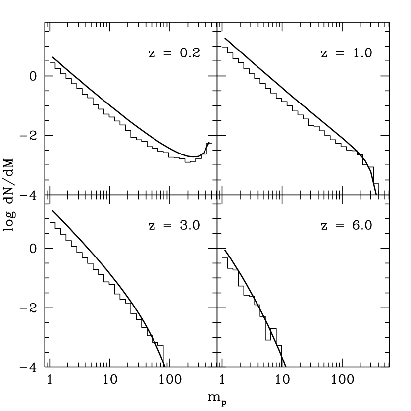
Figure 10: The number of progenitors with mass $M$, for a halo with $M_{0}=500$, using the Binary Tree Method with accretion. Here mergers may involve only two halos with mass greater than $M_{l}$, but an indefinite number of mergers with halos with mass smaller than $M_{l}$ (accretion). As usual the solid line is the extended Press-Schechter prediction. The trees (histograms) now underproduce halos compared to the Press-Schechter model.

The results for the conditional mass function of a single halo are shown in Figure 10. The discrepancy is now in the opposite direction: the number of halos is underpredicted relative to the extended Press-Schechter prediction. Apparently this procedure now overestimates the accreted mass. This is not too surprising since we allowed large amounts of mass to be designated as accreted mass simply because two progenitors had already been found. It appears that even in the limit of small time steps and for large mass halos, mergers between more than two halos cannot be neglected. In some ways this is not surprising either, because after all the division into $M>M_{l}$ and $M<M_{l}$ is arbitrary and has no physical basis.

6.3 The Successful Method: $N$-Branch Trees With Accretion

It is trivial to generalize our previous recipe to allow an unrestricted number of progenitors. We now continue picking progenitor masses until the unallocated mass $\Delta M$ is less than $M_{l}$. This is indicated on the flow-chart by the dashed line labeled “To ${\cal P}_{3}$”. Note that the total accreted mass can still exceed $M_{l}$ because some of the attempts to pick progenitors yield halos with $M<M_{l}$ and contribute to the accreted mass. We still pick the time-step so that the number of progenitors cannot get too large (we find that we never exceed ten progenitors per time step even for cluster mass halos ($M_{0}=5\times 10^{4}\,M_{l}$)). We find a good compromise between efficiency and accuracy if we introduce an additional scaling in the expression for $\Delta\omega$ from Eqn. 23, of the form $b+a\log_{10}(M/M_{l})$, where we have used the parameters $a=0.3$ and $b=0.8$ for the results shown here. This optimal scaling would change for a different power spectrum shape.

Figure 12: The number of progenitors with mass $M$, for a halo with initial mass $M_{0}$, using the $N$-Branch Tree Method with accretion. This is the same as the binary tree method with accretion except that an arbitrary number of progenitors is allowed at each branching. The solid line is the extended Press-Schechter prediction. (a) $M_{0}=5\>M_{l}$ (b) $M_{0}=500\>M_{l}$ (c) $M_{0}=5\times 10^{4}\>M_{l}$. The merger trees (histograms) are in reasonably good agreement with the extended Press-Schechter model.

This recipe gives good results for the conditional mass function for parent halos with a wide range of masses. We show this in Figure 12 for parent halos with $M_{0}=5\,M_{l},500\,M_{l}$ and $5\times 10^{4}\,M_{l}$. The agreement is poorest for halos with $M_{0}\mathrel{\hbox{\hbox to0.0pt{\hbox{\lower 4.0pt\hbox{$\sim$}}\hss}\hbox{$<$}}}10\,M_{l}$. If we require strict mass conservation, this is an unavoidable problem due to the shape of the conditional mass function for halos of this size. This should be kept in mind when setting the value of $M_{l}$ — it should be chosen such that only objects larger than $\sim 10M_{l}$ correspond to observable galaxies. We also check the mass weighted quantity $\bar{f}_{p}$, the fraction of mass in progenitors as a function of redshift. This is shown in Figure 14.

Figure 14: The average fraction of the original mass $M_{0}$ contained in progenitors (halos with $M>M_{l}$) at a redshift $z$. The solid line shows the prediction of the Press-Schechter model. The square symbols show the average given by the merger trees ($N$-Branch Tree Method with accretion) Error bars show the standard deviation ($1\sigma$) over many ensembles.

This quantity shows good agreement for the smallest halo, $M_{0}=5\,M_{l}$, which shows that the accreted mass is being treated properly, so that we do not need to worry about the less than perfect agreement in the conditional mass function, as long as the condition on $M_{l}$ mentioned above is satisfied. Note that the agreement of the mass function can be improved by adjusting the time-step, but at the expense of $\bar{f}_{p}$. We adjust the time-step to achieve the best possible agreement for both the number and mass weighted quantities, over the entire mass range. We compute the universal mass function from the weighted grid of merging histories constructed using our new scheme, and plot this in Figure 16. We now find very good agreement with the prediction of the standard Press-Schechter theory.

Figure 16: The total mass function obtained from the $N$-Branch Tree Method with accretion (the successful method). The solid lines show the prediction of the Press-Schechter theory, at $z=0.16$, 2.5, 3.6, 5 and 7 from top to bottom. Broken histograms show the mass function from the merger trees, constructed as described in Fig. 6.

We therefore conclude that although this method is not rigorous, it produces acceptable agreement with the mean quantities that we can check with the Press-Schechter model.

7 The Number-Mass Distribution of Progenitors

We have now developed a convenient and efficient method for constructing merger trees. The averages derived from an ensemble of these trees agree with the important mean quantities predicted by the extended Press-Schechter theory. However, part of the motivation for developing this new method was to ensure that the ensemble obeys the true joint probability distribution. We have not yet shown this to be the case, and we have already mentioned the lack of any information from the standard Press-Schechter formalism which would allow us to evaluate the Monte Carlo trees against analytic predictions.

Figure 18: The probability distribution of the number of progenitors, for a parent halo with mass $M_{0}$ at several redshifts. The histogram shows the results from the Monte Carlo merging trees (N-Branch Tree Method with accretion). The stars show the results of the semi-analytic model developed in section 5. Left panel: $M_{0}=5\>M_{l}$. Right Panel: $M_{0}=50\>M_{l}$

We do have the predictions of the model we developed in section 5, but we do not trust them for reasons discussed in that section. However, out of curiosity we compare the predictions of the semi-analytic accretion model for the probability distribution of the number of progenitors, ${\cal P}_{N}$, with the results of the Monte Carlo merger trees. The integrals were performed numerically using a recursive, adaptive stepsize Runga-Kutta algorithm. Figure 18 shows the ${\cal P}_{N}$ distributions for halos with mass $M_{0}=5$ and $M_{0}=50$ at redshifts of 0.1, 0.2, 1, and 3. The results agree rather well for redshift steps of $\Delta z=0.2$ or smaller. For larger steps in redshift, the semi-analytic results do not agree as well, probably due to the breakdown of the accretion model.

Figure 20: The evolution with redshift of the two-dimensional distribution of the number of progenitors and their masses for a halo of mass $M_{0}$, obtained from Monte Carlo realizations of the $N$-Branch Merger Trees with accretion. (a) $M_{0}=5\>M_{l}$ (b) $M_{0}=50\>M_{l}$ (c) $M_{0}=500\>M_{l}$. These figures are available by anonymous ftp from ftp.ucolick.org (pub/outgoing/rachel).

Figure 20 demonstrates the importance of taking into account the joint distribution in the progenitor number – progenitor mass space. The figure shows strong correlations between the two variables. Some of the correlations are obvious: in Figure 20a, we show the distribution for a parent halo of $M_{0}=5\,M_{l}$. In the first redshift step ($z_{0}=0$, $z_{1}=0.2$) the highest probability is obtained for having a single progenitor, and this progenitor naturally contains a large fraction of the mass $M_{0}$. As we progress in redshift, this correspondence is not preserved. Accreted mass starts to be more and more significant, and the unseen accreted mass complements low mass progenitors so that the sum may reach $M_{0}$. At the formation epoch of $M_{0}$, all ${\cal P}_{N}$ are populated, and in earlier stages most of the halos go below $M_{l}$, when the dominant process is of single progenitors that accumulate accreted mass. It is interesting to notice that the “formation epoch” (the earliest time when the largest progenitor has mass greater than $M_{0}/2$) is not dominated by mergers of equal mass halos, but rather approached via slow accretion. This general picture also remains valid for higher $M_{0}$ (Figure 20b and c): an increase in the number of progenitors occurs towards an intermediate redshift, and it then declines towards containing most of the mass in the accreted component. However it should be noted that the highest mass considered here would be comparable to the halo of a Milky Way sized galaxy ($5\times 10^{12}\mbox{$M_{\odot}$}$). For much larger mass halos (comparable to group or cluster mass halos), accretion is less important relative to the aggregation of roughly equal mass progenitors.

The probability for the number of progenitors spans substantial parts of its permitted range even for $M_{0}=500$. It is therefore clear why an infinitesimal step is needed for the two-progenitor scheme to work. As soon as we consider a finite timestep, the probability for ${\cal P}_{N>2}$ is no longer negligible.

The details of the redshift sequence represent the characteristics of the specific power spectrum and cosmology we used for the Monte-Carlo realization. The formation time as a function of halo mass and redshift are determined by the cosmology and the power spectrum. The qualitative trend of this sequence, however, is similar for all cosmologies and all hierarchical power spectra.

Figure 20 suggests that the progenitor mass and number distribution functions are an interesting avenue to pursue in the study of structure formation via merger trees. More importantly, it points at the existing interplay between the accreted mass, the progenitor mass and the number of progenitors; an interplay in which none of the three can be treated separately from the other.

8 Summary and Conclusions

We have presented a new method for constructing the merging history of dark matter halos in a semi-analytic way. We have highlighted the need to impose an arbitrary mass cutoff for practical reasons, which leads us to distinguish between halos above and below this threshold as “progenitors” or “accreted mass”, respectively. The scheme we have proposed and implemented treats accreted mass and progenitors in a self consistent way, and produces good agreement with the average quantities predicted by the underlying Press-Schechter theory, such as the conditional and universal mass function of halos and the mean mass in progenitors as a function of redshift.

Our method is an improvement on the method proposed by ?), which, after many steps in redshift, substantially overproduces halos relative to the Press-Schechter mass function. Our work suggests that it is not possible to simultaneously conserve mass exactly and retain the exact agreement with the conditional mass function from the extended Press-Schechter model. The method of ?) reproduces the conditional mass function exactly and conserves mass approximately. Our method conserves mass exactly and reproduces the conditional mass function approximately. This seems to be a necessary trade-off. Our method does have certain practical advantages: it does not require the creation and storage of a large number of ensembles, it is numerically robust, it does not require the imposition of a grid is mass or redshift, and it will work for any power spectrum.

We have pointed out the necessity of investigating the full probability distribution of the number of progenitors and their masses. This cannot be tested within the boundaries of the existing theory, and so must be examined by comparisons with N-body simulations. However, the simulations have their own problems and complications, such as the limitations of mass and spatial resolution and the ambiguities of defining halos, so they should not be regarded as necessarily representing the absolute truth. In addition the agreement between the simulations and the Press-Schechter model is only approximate, even for the mean quantities such as the mass function. It would therefore be desirable to have a reliable theoretical means of addressing this problem. We have attempted to reformulate the extended Press-Schechter theory to obtain the full probability distribution for the number of progenitor halos ${\cal P}_{N}$. Although this model gives qualitatively reasonable results for certain cases, some ingredients remain ad-hoc.

For the moment, this leaves us with no recourse but to appeal to N-body simulations. In a companion paper [Somerville et al. (1998)], we will compare the results we have obtained here with numerical simulations. This comparison has two goals: (a) to determine the quality of agreement of the analytic and Monte Carlo results with the N-body simulation results. (b) to study the full distribution of the various quantities, and determine whether the Monte Carlo method developed here reproduces these results. The merger trees will then be used as the framework for the development of full semi-analytic galaxy formation models, and used to compare with a variety of observations [Somerville (1997), Somerville & Primack (1998)].

References

- Bardeen et al. (1986) Bardeen J. M., Bond J. R., Kaiser N., Szalay A. S., 1986, ApJ, 304, 15 (BBKS)
- Bond et al. (1991) Bond J. R., Cole S., Efstathiou G., Kaiser N., 1991, ApJ, 379, 440
- Bower (1991) Bower R., 1991, MNRAS, 248, 332
- Cole (1991) Cole S., 1991, ApJ, 367, 45
- Cole et al. (1994) Cole S., Aragón-Salamanca A., Frenk C., Navarro J., Zepf S., 1994, MNRAS, 271, 781
- Cole & Kaiser (1988) Cole S., Kaiser N., 1988, MNRAS, 233, 637
- Efstathiou et al. (1992) Efstathiou G., Bond J., White S., 1992, MNRAS, 258, 1
- Efstathiou et al. (1988) Efstathiou G., Frenk C. S., White S. D. M., Davis M., 1988, MNRAS, 235, 715
- Eisenstein & Loeb (1996) Eisenstein D., Loeb A., 1996, ApJ, 459, 432
- Gelb & Bertschinger (1994) Gelb J. M., Bertschinger E., 1994, ApJ, 436, 467
- Gross et al. (1998) Gross M. A. K., Somerville R. S., Primack J. R., Holtzman J., Klypin A. A., 1998, MNRAS, submitted, astro-ph/9712142
- Kauffmann (1996) Kauffmann G., 1996, MNRAS, 281, 487
- Kauffmann & White (1993) Kauffmann G., White S., 1993, MNRAS, 261, 921
- Kauffmann et al. (1993) Kauffmann G., White S., Guiderdoni B., 1993, MNRAS, 264, 201
- Lacey & Cole (1993) Lacey C., Cole S., 1993, MNRAS, 262, 627 (LC93)
- Lacey & Cole (1994) Lacey C., Cole S., 1994, MNRAS, 271, 676
- Ma (1996) Ma C., 1996, ApJ, 471, 13
- Peebles (1980) Peebles P. J. E., 1980, The Large-Scale Structure of the Universe. Princeton Univ. Press, Princeton, NJ
- Press & Schechter (1974) Press W., Schechter P., 1974, ApJ, 187, 425
- Somerville (1997) Somerville R., 1997, Ph.D. thesis, University of California, Santa Cruz, http://www.fiz.huji.ac.il/ rachels/thesis.html
- Somerville et al. (1998) Somerville R., Lemson G., Kolatt T., Dekel A., 1998, in preparation
- Somerville & Primack (1998) Somerville R. S., Primack J. R., 1998, MNRAS, submitted
- White & Frenk (1991) White S., Frenk C., 1991, ApJ, 379, 52