COSMIC MICROWAVE BACKGROUND MAPS FROM THE HACME EXPERIMENT

Abstract

We present Cosmic Microwave Background (CMB) maps from the Santa Barbara HACME balloon experiment (Staren et al. 2000), covering about 1150 square degrees split between two regions in the northern sky, near the stars $\gamma$ Ursae Minoris and $\alpha$ Leonis, respectively. The FWHM of the beam is $\sim 0.77^{\circ}$ in three frequency bands centered on 39, 41 and 43 GHz. The results demonstrate that the thoroughly interconnected scan strategy employed allows efficient removal of $1/f$-noise and slightly variable scan-synchronous offsets. The maps display no striping, and the noise correlations are found to be virtually isotropic, decaying on an angular scale $\sim 1^{\circ}$. The noise performance of the experiment resulted in an upper limit on CMB anisotropy. However, our results demonstrate that atmospheric contamination and other systematics resulting from the circular scanning strategy can be accurately controlled, and bodes well for the planned follow-up experiments BEAST and ACE, since they show that even with the overly cautious assumption that $1/f$-noise and offsets will be as dominant as for HACME, the problems they pose can be readily overcome with the mapmaking algorithm discussed. Our prewhitened notch-filter algorithm for destriping and offset removal should be useful also for other balloon- and ground-based experiments whose scan strategies involve substantial interleaving.

1. INTRODUCTION

One of the main goals of the next generation of Cosmic Microwave Background (CMB) experiments is to produce maps that can resolve degree scale features corresponding to acoustic peaks in the angular power spectrum (see e.g. Bond 1996 and Hu et al. 1997 for reviews), since this potentially allows accurate determination of cosmological parameters (Jungman et al. 1996; Bond et al. 1997; Zaldarriaga et al. 1997).

To date, maps with degree scale angular resolution have been published from the ACME/MAX (White & Bunn 1995), Saskatoon (Tegmark et al. 1997 – hereafter “T97d”), CAT (Jones 1997) and QMAP (Devlin et al. 1998; Herbig et al. 1998; de Oliveira-Costa et al. 1998) and Python (Coble et al. 1999) experiments. The maps we present are based on the 1996 flight of the HACME balloon experiment, which is described in detail by Staren et al. (2000, hereafter “S2000”). They cover regions around the stars $\gamma$ Ursae Minoris ($\gamma$UMi) and $\alpha$ Leonis ($\alpha$Leo), as shown in Figure 1 (the COBE DMR map is from Bennett et al. 1996). The data analysis we describe below is an interesting pathfinder for upcoming mapping experiments since HACME differed from its predecessors ACME/MAX, Saskatoon and CAT in three important ways:

1. The time-ordered data set is substantially larger (consisting of $\sim 10^{7}$ temperature measurements).

2. $1/f$-noise plays a significant role.

3. The scan strategy interconnects the observed pixels in a complicated way.

To use this interconnectedness for efficient $1/f$-noise

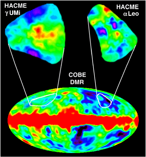
Figure 1.— Location of observing regions in galactic coordinates.

removal, we apply the lossless mapmaking algorithm described in Tegmark (1997a, hereafter “T97a”) tailored to the noise power spectrum at hand. Our analysis provides the first large scale test of this method, since the large size of our data set forces us to use all the numerical tricks that have been proposed for accelerating it (Wright 1996; Tegmark 1997c – hereafter “T97c”). We describe our analysis in Section 2 and present the results in Section 3.

2. METHOD

We make our maps using the minimum-variance method described by Wright (1996), T97a and T97c, which we summarize briefly below.

Let $y_{i}$ denote the temperature measured by the HACME experiment at the $i^{th}$ observation (there were 312.5 such measurements per second), and group this time-ordered data set (TOD) into an $M$-dimensional vector ${\bf y}$. As described in S2000, there are $M=3,323,250$ measurements in the $\gamma$UMi region and 1,743,625 in the $\alpha$Leo region, respectively, for each of the three frequency channels. Discretizing the map into $N$ pixels centered at unit vectors $\widehat{\bf r}_{1},...,\widehat{\bf r}_{N}$, we let $x_{i}$ denote the true beam-smoothed CMB temperature in the direction $\widehat{\bf r}_{i}$ and group these temperatures into an $N$-dimensional map vector ${\bf x}$. The TOD is related to the map by

$${\bf y}={\bf A}{\bf x}+{\bf n},$$ (1)

where ${\bf n}$ denotes a random noise vector and the $M\times N$ matrix ${\bf A}$ encodes the HACME scan strategy. Letting $N_{i}$ denote the number of the pixel pointed to at the $i^{th}$ observation, we have ${\bf A}_{ij}=1$ if $N_{i}=j$, ${\bf A}_{ij}=0$ otherwise, so all the entries of ${\bf A}$ are zero except that there is a single “1” in each row. We find that ${\bf n}$ can be accurately modeled as a multivariate Gaussian random variable with zero mean ($\langle{\bf n}\rangle={\bf 0}$), so it is completely specified by its covariance matrix ${\bf N}\equiv\langle{\bf n}{\bf n}^{t}\rangle$.

The problem at hand is to compute a map $\tilde{\bf x}$ that estimates the true map ${\bf x}$ using the TOD ${\bf y}$. As shown in T97a, all the cosmological information from the TOD is retained in the map $\tilde{\bf x}$ given by

$$\tilde{\bf x}=[{\bf A}^{t}{\bf M}{\bf A}]^{-1}{\bf A}^{t}{\bf M}{\bf y},$$ (2)

where the matrix ${\bf M}\equiv{\bf N}^{-1}$. Substituting this into equation (1) shows that we can write $\tilde{\bf x}={\bf x}+\hbox{\bfmath\char 34\relax}$, i.e., that our map estimate $\tilde{\bf x}$ equals the true map ${\bf x}$ plus a Gaussian noise term ” that is independent of ${\bf x}$. This holds for any choice of ${\bf M}$. This pixel noise has zero mean ($\langle\hbox{\bfmath\char 34\relax}\rangle={\bf 0}$) and a covariance matrix given by

$${\bf\Sigma}\equiv\langle\hbox{\bfmath\char 34\relax}\hbox{\bfmath\char 34\relax}^{t}\rangle=[{\bf A}^{t}{\bf M}{\bf A}]^{-1}[{\bf A}^{t}{\bf N}^{-1}{\bf A}][{\bf A}^{t}{\bf M}{\bf A}]^{-1}.$$ (3)

To minimize the noise, we want to choose ${\bf M}\approx{\bf N}^{-1}$ (at least approximately), which gives ${\bf\Sigma}$ near the best possible case $[{\bf A}^{t}{\bf N}^{-1}{\bf A}]^{-1}$. For the simple case of white noise from the detector, we would have ${\bf N}\propto{\bf I}$, the identity matrix, and $\tilde{\bf x}$ would be obtained by simply averaging the measurements of each pixel in the map. We will refer to this as the straight averaging mapmaking method, in contrast to the prescription of equation (2), which we will call the minimum noise method. In our case, the matrix ${\bf N}$ is far from diagonal, since long-term $1/f$ drifts introduce correlations between the noise $n_{i}$ at different times. To eliminate the need for a numerically unfeasible inversion of ${\bf N}$ in equations (2) and (3), we employ the prewhitening trick of Wright (1996) and define a new data set $\tilde{\bf y}\equiv{\bf D}{\bf y}$, where the prewhitening matrix ${\bf D}$ is chosen so that the prewhitened noise $\tilde{\bf n}\equiv{\bf D}{\bf n}$ becomes as close to possible to white noise, i.e., so that the filtered noise covariance matrix $\tilde{\bf N}\equiv\langle\tilde{\bf n}\tilde{\bf n}^{t}\rangle={\bf D}{\bf N}{\bf D}^{t}\approx{\bf I}$. Defining $\tilde{\bf A}\equiv{\bf D}{\bf A}$, this allows us to rewrite equation (1) as $\tilde{\bf y}=\tilde{\bf A}{\bf x}+\tilde{\bf n}$, so equations (2) and (3) give

$$\tilde{\bf x} = [\tilde{\bf A}^{t}{\bf M}\tilde{\bf A}]^{-1}\tilde{\bf A}^{t}{\bf M}\tilde{\bf y}$$ (4)

$$= [{\bf A}^{t}{\bf D}^{t}{\bf M}{\bf D}{\bf A}]^{-1}{\bf A}^{t}{\bf D}^{t}{\bf M}{\bf D}{\bf y},$$

$${\bf\Sigma} = [{\bf A}^{t}{\bf D}^{t}{\bf M}{\bf D}{\bf A}]^{-1}[{\bf A}^{t}{\bf D}^{t}{\bf M}\tilde{\bf N}{\bf M}^{t}{\bf D}{\bf A}][{\bf A}^{t}{\bf D}^{t}{\bf M}{\bf D}{\bf A}]^{-1},$$

where we make the choice ${\bf M}\equiv{\bf I}$ since $\tilde{\bf N}\approx{\bf I}$. To accelerate the numerical evaluation of these expressions, we take advantage of the fact that ${\bf D}^{t}{\bf D}$ is almost a circulant matrix, as described in detail in T97c. Since the statistical properties of the noise are approximately constant over time (the covariance $\langle n_{i}n_{j}\rangle$ depends only on the time interval $|i-j|$ between the two observations), the prewhitening filter ${\bf D}$ is simply a convolution filter. We compute it as described in T97a, and the result is plotted in Figure 2. The prewhitening procedure renders the data insensitive to the mean (monopole) of the map. This makes the matrix $[\tilde{\bf A}^{t}{\bf M}\tilde{\bf A}]$ non-invertible, which is remedied using the pseudo-inverse technique described in the Appendix of Tegmark (1997b).

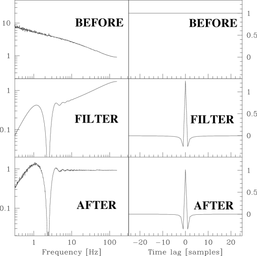
Figure 2.— The prewhitening procedure is illustrated in the frequency domain (left) and in the time domain (right) for the $\gamma$UMi 43 GHz channel. The noise power spectrum (upper left) contains a $1/f$-component which causes the noise to be almost perfectly correlated between measurements close together in time (upper right). By multiplying the Fourier transformed signal by an appropriate prewhitening filter (middle left), which corresponds to applying a convolution filter (middle right) to the signal, the filtered TOD $\tilde{\bf y}$ obtains a noise power spectrum which is close to white noise with notches at 0 Hz and the spin frequency (lower left), corresponding to a time autocorrelation function that falls of rapidly (lower right).

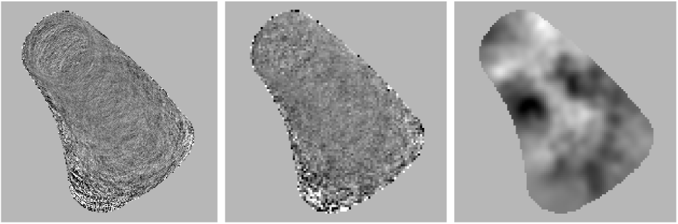
Figure 3.— Straight averaging (left), optimal unsmoothed (center) and Wiener filtered (right) maps of the $\alpha$Leo region at 43 GHz.

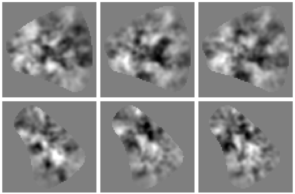
Figure 4.— Wiener-filtered maps of the $\gamma$UMi (top) and $\alpha$Leo (bottom) regions at 39 GHz (left), 41 GHz (center) and 43 GHz (right).

In addition to the map $\tilde{\bf x}$, we also compute the Wiener filtered map ${\bf x}_{w}$, which is given by (Wiener 1949)

$${\bf x}_{w}\equiv{\bf S}[{\bf S}+{\bf N}]^{-1}\tilde{\bf x},$$ (5)

where the CMB signal covariance matrix ${\bf S}\equiv\langle{\bf x}{\bf x}^{t}\rangle$ is given by the standard formula

$${\bf S}_{ij}=\sum_{\l=2}^{\infty}{(2\l+1)\over 4\pi}P_{\l}(\widehat{\bf r}_{i}\cdot\widehat{\bf r}_{j})B_{\l}^{2}C_{\l}$$ (6)

for some assumed fiducial power spectrum $C_{\l}$. In our analysis, we approximate the HACME beam as a circular FWHM$=0.77^{\circ}$ Gaussian, although the actual beam has an asymmetry of order 6%. Thus $B_{\l}\approx e^{-\theta^{2}\l(\l+1)/2}$, where $\theta\equiv(8\ln 2)^{-1/2}$ FWHM. As discussed in T97a, the Wiener filtered map ${\bf x}_{w}$ contains the same cosmological information as $\tilde{\bf x}$ (which we will refer to as the unsmoothed map to distinguish it from ${\bf x}_{w}$), but is more useful for visual inspection since it is less noisy. Wiener filtering has been successfully applied to both CMB maps (e.g., Bunn et al. 1994, 1996; T97d) and galaxy surveys (e.g., Fisher et al. 1995; Lahav et al. 1994; Zaroubi et al. 1995).

After removal of calibration data from ${\bf z}$, segments during which control commands were transmitted to the gondola are omitted, which reduces the size of the TOD by about $0.4\%$. The remainder has scan-synchronous offsets described in S2000. We determine the time-independent scan- synchronous component simultaneously with the map by including unknown offsets, one corresponding to each of the 125 sampling positions along the circular scan, as 125 additional “pixels” in the vector ${\bf x}$ and widening ${\bf A}$ accordingly with an additional “1” in each row. This trick was subsequently applied also in the analysis of QMAP — see de Oliveira-Costa et al. (1998).

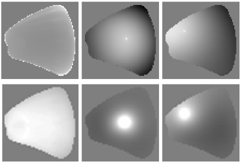
Figure 5.— Noise properties of the unsmoothed (top) and Wiener filtered (bottom) $\gamma$UMi maps at 43 GHz. The leftmost maps show the rms noise in each pixel. The remaining maps show the correlations with two typical pixels, located at the centers of the white dots.

3. RESULTS

3.1. 1/f-noise removal

Figure 3 (left panel) shows the 43 GHz $\alpha$Leo map obtained with the straight averaging method (simply averaging the observations of each pixel), and illustrates why the more sophisticated minimum noise method (middle panel) is needed. The visible striping along the circular scans (see S2000 for details about the scan pattern) is caused by $1/f$-noise, which creates strong correlations between map pixels that are scanned within a short time of one another. The middle panel shows that our improved mapmaking technique has eliminated this striping. This is more vividly illustrated in Figure 5 (upper right panels), showing two typical rows of the noise covariance matrix ${\bf\Sigma}$. Since row $i$ gives the correlations to $i^{th}$ pixel, the small round white dots tell us that strong noise correlations persist only between pixels that are close neighbors. Moreover, these correlations are seen to be quite isotropic, with no signs of elongation along scan directions (the only exceptions are pixels close to edges). There is a slight anticorrelation to very distant pixels caused by the above-mentioned monopole removal, which forces the correlation map to have a vanishing average. This removal of 1/f-noise also causes a substantial reduction in the rms pixel noise (upper left panel in Figure 5), which is about a factor of two lower than for the straight averaging map. Both of these desirable properties of the pixel noise can be readily understood by comparing our scan strategy to the four toy models described in T97c. Since the circular HACME scans cross one another at virtually every pixel, the geometry is similar to the “fence pattern”, which was found to produce isotropic noise correlations like those in Figure 5. A “fence” map made with the straight averaging method would correlate the noise in a pixel with neighbors along the two perpendicular scan directions, which form a “+”-shaped region around the pixel. With the minimum-noise method, on the other hand, a pixel is linked to all its neighbors via a sequence of intersecting scans in a zig-zag pattern. This is accomplished automatically in the matrix inversion step, and has the effect of isotropizing correlations (thereby reducing long-range correlations) and utilizing the available information better (reducing the resulting pixel noise).

3.2. Wiener-filtered maps

The rms pixel noise $\sigma_{i}\equiv{\bf\Sigma}_{ii}^{1/2}$ in the unsmoothed 43 GHz $\alpha$Leo map (middle panel of Figure 3) is about $400\>{\rm\mu K}$ per $(0.3^{\circ})^{2}$ pixel in the central parts and $250\>{\rm\mu K}$ when rebinned into $(0.8^{\circ})^{2}$ pixels, i.e., substantially larger than any expected CMB signal. What the eye perceives is therefore mostly noise, so it is desirable to increase the signal-to-noise ratio by smoothing. Moreover, some pixels near the edges are extremely noisy (with an rms around $10\>{\rm mK}$) since they were only observed a small number of times (upper left panel of Figure 5). To prevent them from dominating the image, it is desirable to give them less weight. The Wiener filtered map (right panel of Figure 3) automatically remedies both of these problems. The new noise map (lower left panel of Figure 5) shows that the noise explosion near the edges has been eliminated, and the new correlation maps (lower right panels of Figure 5) show that smoothing has widened the correlated region. To avoid imprinting features on any particular angular scale, we have used a flat fiducial power spectrum $C_{\l}=24\pi Q^{2}/5\l(\l+1)$ in equation (6) just as in T97d, normalized to $Q=30{\rm\mu K}$. Figure 4 shows the Wiener-filtered $\gamma$UMi and $\alpha$Leo maps for all three channels, on a symmetric linear grey scale from low (black) to high (white) temperatures. Since some maps are substantially noisier than others and the Wiener filtering suppresses their temperature scale accordingly, the grey scale has been separately normalized for each map to avoid saturation and allow direct comparison of spatial morphology.

3.3. Verification and testing

We tested our data-analysis pipeline by generating mock sky maps that were observed with the actual HACME scan pattern. These simulated TOD sets were then run through the pipeline, recovering the original maps. When adding noise to the TOD with the measured HACME power spectrum, the pixel noise in the recovered map was found to be fully consistent with the noise covariance matrix ${\bf\Sigma}$ computed by the pipeline.

To test if the reconstructed map was sensitive to the pixel size, the analysis was repeated for a range of pixel sizes. As expected, this produced virtually identical maps, as long as the pixel size was smaller than the $0.77^{\circ}$ beam size by at least the Shannon oversampling factor $2.5$.

To test if the Wiener-filtered maps were sensitive to the choice of fiducial band power, they were computed for the band power normalizations $Q=20$, $30$ and $40\,{\rm\mu K}$. The visual difference between the two extreme cases was minimal, corresponding merely to an increase in the effective smoothing scale by about $10\%$ (for more details on why this is expected, see the discussion in T97d).

3.4. Constraints on systematics and the CMB power spectrum

The initial version of our analysis assumed that the scan-synchronous offsets were time-independent. The result was a marginal detection of fluctuations in the most sensitive channel (43 GHz) and upper limits at 39 and 41 GHz. However, subsequent tests showed that variations in these offsets at the level of a few percent could masquerade as signal at this level. Since the offsets are completely dominated by the first harmonic (at the scan frequency), we repeated the entire analysis after throwing away all the information about this frequency. This corresponded to replacing the whitening filter $D$ discussed in Section 2 by a notch filter that vanished at this frequency (as well as at 0 Hz). The Wiener-filtered maps shown in Figures 1 and 3 were made without the notch filter, whereas those in Figure 4 used it. The result of the notch filter was an increase in the rms noise of about 50% for the least noisy pixels in the raw maps, as well as a reduction of the signal seen to levels that were no longer statistically significant. The pixel noise $\sigma_{i}$ (from detector noise only) is $385\,{\rm\mu K}$ in the best pixel in the 43 GHz map of the $\gamma$UMi region, The 41 and 39 GHz channels are noisier by factors of 1.2 and 1.9, respectively. For comparison, a CDM-like power spectrum normalized to a band power $Q_{\rm flat}=30,{\rm\mu K}$ would give corresponding pixel fluctuations of order $80\,{\rm\mu K}$ in the this map including the mean removal. Most of the fluctuations seen in the raw maps are therefore noise rather than sky signal, and as described below, this remains true for the Wiener-filtered maps as well. The reason that many features are seen to recur between the channels is that their noise is correlated. Although there is a slight sensitivity to the dipole (with sky rotation marginally breaking the degeneracy between the scan-synchronous offset and the dipole), the resulting noise error bars on this mode are too large to allow a detection after our notch filtering.

To place quantitative constraints on the systematics and sky signal in the maps, we perform a signal-to-noise eigenmode analysis (Bond 1994; Bunn & Sugiyama 1995). We define a new data vector

$${\bf y}\equiv{\bf B}^{t}{\bf x},$$ (7)

where ${\bf b}$, the columns of the matrix ${\bf B}$, are the eigenvectors of the generalized eigenvalue problem

$${\bf S}{\bf b}=\lambda{\bf\Sigma}{\bf b},$$ (8)

sorted from highest to lowest eigenvalue $\lambda$ and normalized so that ${\bf b}^{t}{\bf N}{\bf b}={\bf I}$. A sample of eigenmodes ${\bf b}$ are shown in Figure 6, and the corresponding expansion coefficients $y_{i}$ are plotted in Figure 7. If there are no systematic errors or residual offset problems, detector noise should contribute uncorrelated fluctuations of unit variance to each mode. All systematic problems we have considered would add rather than subtract map power. Figure 7 indeed shows no evidence of outliers or other problems with our noise model.

The covariance of the expansion coefficients is $\langle y_{i}y_{j}\rangle=\delta_{ij}(1+\lambda_{i})$, so cosmic signal at the assumed level would boost the variance somewhat. The very best 43 GHz $\gamma$UMi mode $(i=1)$ has $\lambda_{i}\approx 0.32$, corresponding to an expected rms of $(1+\lambda_{i})^{1/2}\approx 1.15$ for $y_{i}$. Figure 7 is seen to be quite consistent with this. Thus no single mode has signal-to-noise exceeding unity.

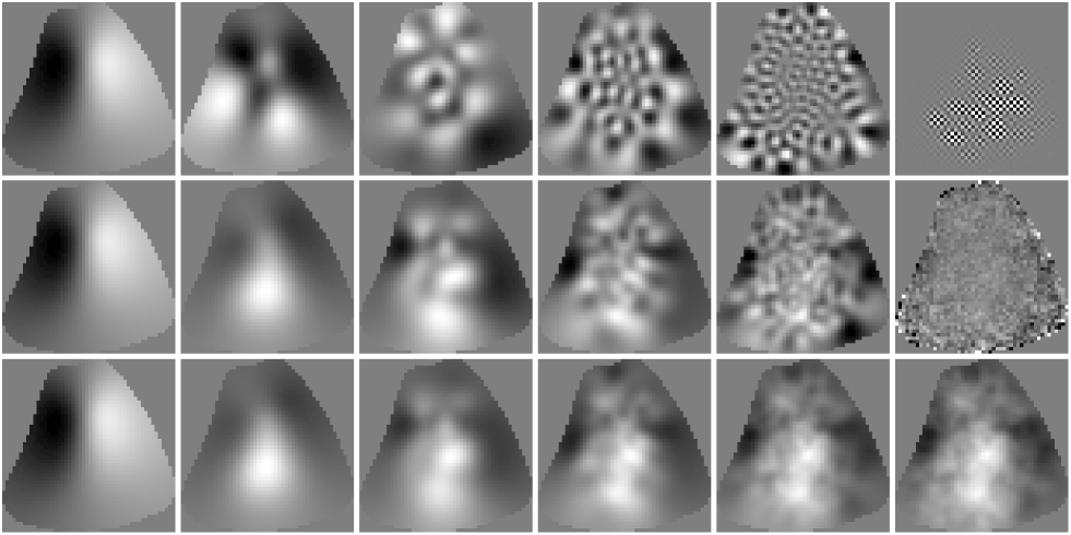
Figure 6.— The top row shows a S/N eigenmodes number 1, 3, 10, 100, 300 and 3082 for the 43 GHz $\gamma$UMi map, which are seen to probe successively smaller (and noisier) scales. The second row shows cumulative sums up to these mode numbers, with each mode weighted by its expansion coefficient so that the total sum recovers the original map (right). The last row shows the analogous running sums with the $i^{th}$ coefficient rescaled by $\lambda_{i}/(\lambda_{i}+1)$, so that the total sum recovers the Wiener- filtered map (right).

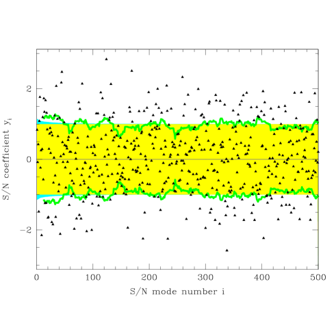
Figure 7.— The triangles show the first 500 S/N eigenmode expansion coefficients $y_{i}$ for the 43 GHz $\gamma$UMi map. If there were no systematics or CMB fluctuations in the map, merely detector noise, they would have unit variance, and about $68\%$ of them would would be expected to lie within the yellow/light grey band. For a flat $Q_{\rm flat}=30\,\mu$K CMB power spectrum, the standard deviation would be larger for the best modes, as indicated by the thin blue/grey band on the left side. The wiggly green/grey curve is the rms of the data points $y_{i}$, averaged in bands of width 25.

To place cosmological constraints, we need to combine the information from all modes. We do this using the decorrelated quadratic estimator method described in Tegmark (1997b). We find that no channel gives a statistically significant detection. The sharpest upper limit comes from the 43 GHz $\gamma$UMi data, giving $\delta T\equiv[\l(\l+1)C_{\l}/2\pi]^{1/2}<77\,{\rm\mu K}$ at 95% confidence with the window function shown in Figure 8. This corresponds to the effective angular scale $\l=38^{+25}_{-20}$.

What was the price paid for using the notch filter? Figure 8 shows that this destroys information on scales $\ell\mathrel{\hbox to0.0pt{\lower 3.0pt\hbox{$\mathchar 536\relax$}\hss}\raise 2.0pt\hbox{$\mathchar 316\relax$}}20$, so the 50% increase in rms pixel noise that we found above is caused largely by increased detector noise fluctuations on these large angular scales, comparable to the size of the basic $10^{\circ}$ scanning circle.

Figure 8.— The window functions are shown for the analysis with (solid) and without (dashed) the notch filter. The latter is seen to destroy sensitivity on scales $\ell\mathrel{\hbox to0.0pt{\lower 3.0pt\hbox{$\mathchar 536\relax$}\hss}\raise 2.0pt\hbox{$\mathchar 316\relax$}}20$.

4. CONCLUSIONS

We have presented CMB maps from the HACME balloon experiment, which was devised as a pathfinder for the long-duration balloon experiments BEAST and ACE. Our analysis has clearly demonstrated that neither substantial $1/f$-noise nor slightly variable scan-synchronous offsets are “show-stoppers”, but can be efficiently dealt with using the matrix-based minimum variance notch filter technique. However, to provide interesting cosmological constraints, the raw sensitivity needs to be substantially improved over the HACME pathfinder specifications. Comparing this with the straight averaging method (averaging the observations of each pixel), we found that our analysis technique improved the results in two ways:

1. The resulting rms noise in the maps is reduced by about a factor of two, the equivalent of four times more flight time.

2. Long-range anisotropic noise correlations (“striping”) is virtually eliminated from the maps.

This bodes well for upcoming spin-chopped total power experiments such as BEAST and ACE. BEAST is anticipated to have nearly 3 times higher sensitivity in ${\rm\mu K}\>{\rm s}^{1/2}$ and 2-6 times the angular resolution, with the same ratio of $1/f$ knee to spin rate as HACME and 50 times more integration time. Indeed, the notch filter approach should be useful for any ground- or balloon-based CMB experiment using an interconnected scan-strategy.

Support for this work was provided by NASA through grants NAG5-6034 and NAGW-1062 and through a Hubble Fellowship, HF-01084.01-96A, awarded by the Space Telescope Science Institute, which is operated by AURA, Inc. under NASA contract NAS5-26555, and by the NSF Center for Particle Astrophysics. JWS was supported by GSRP grant NGW-51381. N.F. was partially supported by CNPq and CAPES.

REFERENCES

Bennett, C. L. 1996, ApJ, 464, L1

Bond, J. R. in Cosmology and Large Scale Structure, Les Houches Section LX, ed. R. Schaeffer, J. Silk, M. Spiro, and J. Zinn-Justin 469 (Elsevier, Amsterdam, 1996), p469.

Bond, J. R., Efstathiou, G., & Tegmark, M. 1997, MNRAS, 291, L33

Bunn, E. F. et al. 1994, ApJ, 432, L75

Coble, K. A. 1999, astro-ph/9911419

de Oliveira-Costa, A., Devlin, M., Herbig, T., Miller, A. D., Netterfield, C. B., Page, L. A., & Tegmark, M. 1998, ApJL, 509, L77

Devlin, M., de Oliveira-Costa, A., Herbig, T., Miller, A. D., Netterfield, C. B., Page, L. A., & Tegmark, M. 1998, ApJL, 509, L69

Fisher, K. B. et al. 1995, MNRAS, 272, 885

Herbig, T., de Oliveira-Costa, A., Devlin, M., Miller, A. D., Page, L. A., & Tegmark, M. 1998, ApJL, 509, L73

Hu, W., Sugiyama, N. & Silk, J. 1997, Nature, 386, 37

Jones, M. E. 1997, preprint astro-ph/9611212.

Jungman, G.. Kamionkowski, M., Kosowsky, A & Spergel, D. N. 1996, Phys. Rev. D, 54, 1332

Lahav, O. et al. 1994, ApJ, 423, L93

Netterfield, C. B. et al. 1997, ApJ, 474, 47

Rybicki, G. B. & Press, W. H. 1992, ApJ, 398, 169

Staren, J. et al. 2000, astro-ph/9912212 (“S2000”)

Tegmark, M. 1997a, ApJL, 480, L87 (“T97a”)

Tegmark, M. 1997b, Phys. Rev. D, 55, 5895

Tegmark, M. 1997c, Phys. Rev. D, 56, 4514 (“T97c”)

Tegmark, M., de Oliveira-Costa, A., Devlin, M. J., Netterfield, C. B, Page, L. & Wollack, E. J. 1997, ApJL, 474, L77 (“T97d”)

White, M. & Bunn, E.F. 1995, ApJ, 443, L53

Wiener, N. 1949, Extrapolation and Smoothing of Stationary Time Series (NY: Wiley).

Wright, E. L. 1996, preprint astro-ph/9612006.

Zaldarriaga, M., Spergel, D., & Seljak, U. 1997, ApJ, 488, 1

Zaroubi, S. et al. 1995, ApJ, 449, 446