Scale-invariance of galaxy clustering

Abstract

Some years ago we proposed a new approach to the analysis of galaxy and cluster correlations based on the concepts and methods of modern statistical Physics. This led to the surprising result that galaxy correlations are fractal and not homogeneous up to the limits of the available catalogs. The usual statistical methods, which are based on the assumption of homogeneity, are therefore inconsistent for all the length scales probed so far, and a new, more general, conceptual framework is necessary to identify the real physical properties of these structures. In the last few years the 3-d catalogs have been significatively improved and we have extended our methods to the analysis of number counts and angular catalogs. This has led to a complete analysis of all the available data that we present in this review. In particular we discuss the properties of the following catalogs: CfA, Perseus-Pisces, SSRS, IRAS, LEDA, APM-Stromlo, Las Campanas and ESP for galaxies and Abell and ACO for galaxy clusters. The result is that galaxy structures are highly irregular and self-similar: all the available data are consistent with each other and show fractal correlations (with dimension $D\simeq 2$) up to the deepest scales probed so far ($1000h^{-1}Mpc$) and even more as indicated from the new interpretation of the number counts. The evidence for scale-invariance of galaxy clustering is very strong up to $150h^{-1}Mpc$ due to the statistical robustness of the data but becomes progressively weaker (statistically) at larger distances due to the limited data. In addition the luminosity distribution is correlated with the space distribution in a specific way. These facts lead to fascinating conceptual implications about our knowledge of the universe and to a new scenario for the theoretical challenge in this field.

, and

PACS: 02.50.+s; 98.60.-a; 98.60.Eg

1 Introduction

The four most important experimental evidences of modern Cosmology are: - The space distribution of galaxies and clusters: the recent availability of several three dimensional samples of galaxies and clusters permits the direct characterization of their correlation properties. - The cosmic microwave background radiation (CMBR), that shows an extraordinary isotropy and an almost perfect black body spectrum. - The linearity of the redshift-distance relation, usually known as the Hubble law. This law has been established by measuring independently the redshift and the distance of galaxies. The relation with velocity and space expansion is not tested directly and comes from the theoretical interpretation. - The abundance of light elements in the universe that presents the most stringent evidence of generating and destroying atomic nuclei.

Each of these four points provides an independent experimental fact. The objective of a theory should be to provide a coherent explanation of all these facts together and to explain their interconnections. Our work refers mainly to the first point, the space distribution of galaxies and clusters (Fig.1)

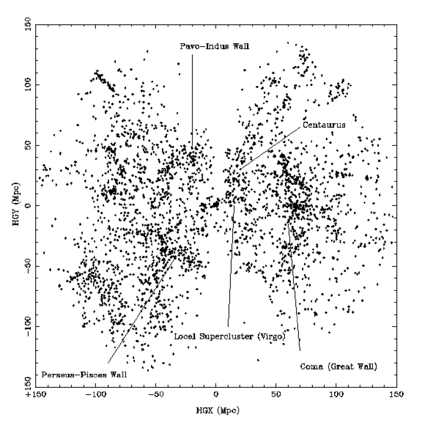
Figure 1: Face-on view of the hypergalactic plane, slice of $150h^{-1}Mpc$ on the Z axis from the LEDA database. Each point corresponds to a galaxy, ours being located at the origins of the coordinates. Our position is in the border with respect to the Local Supercluster centered on Virgo cluster. Artifacts of observations are clearly seen: zones without galaxy radial velocity because of the Milky Way extinction (vertical trace) and radial elongation of galaxy clusters (particularly in periphery). The Local Supercluster seems to be surrounded by an empty region, with a belt made of the neighbor superclusters: Centaurus, Pavo-Indus, Perseus-Pisces and the Great Wall. Voids are filled up due to a projection effect. (Courtesy of H. Di Nella).

which, however, is closely related to the interpretation of all the other points. In particular we claim that the usual methods of analysis are intrinsically inconsistent with respect to the properties of the available samples. The correct statistical analysis of the experimental data, performed with the methods of modern Statistical Physics, shows that the distribution of galaxies is fractal up to the deepest observed scales [1, 2]. This result has caused a strong opposition from various authors in the field because it is in contrast with the usual assumption of large scale homogeneity which is at the basis of most theories. Actually homogeneity represents much more than a working hypothesis for theory, it is often considered as a paradigm or principle and for some authors it is conceptually absurd even to question it [3]. For other authors instead homogeneity is just the simplest working hypothesis and the idea that nature might actually be more complex is considered as extremely interesting [4]. The two points of view are not so different after all because, if something considered absurd becomes real, then it must be really exciting. Given this situation, it may be interesting to analyze why this question develops such strong feelings. This helps us to distinguish opinions from bare facts and to place the discussion in the appropriate perspective.

Figure 2: Example of analytical and non-analytic structures. Top panels: (Left) A cluster in a homogeneous distribution. (Right) Density profile. In this case the fluctuation corresponds to an enhancement of a factor 3 with respect to the average density. Bottom panels: (Left) Fractal distribution in the two dimensional Euclidean space. (Right) Density profile. In this case the fluctuations are non-analytical and there is no reference value, i.e. the average density. The average density scales as a power law from any occupied point of the structure.

The consensus on the homogeneity has never been quite broad. Early works of Kant and Lambert suggested a hierarchy of stars forming clusters forming galaxies which conform larger structures and so on. Fournier d’Albe and Charlier [5, 6] discussed a hierarchy where the mass within distance $d$ varies as $M\sim d$. De Vaucouleurs [7, 8] studied the possibility that there is a universal density-radius power law as a basic factor in Cosmology, reflecting a hierarchic distribution. The hierarchical distribution proposed by De Vaucouleurs can be naturally developed within the framework of fractal geometry. From the theoretical point of view we refer to [9] for a summary of different theoretical approaches to this problem (see also the last section). Interesting discussions about the case of hierarchical distributions of large scale structures can be found in [10] and in [11].

Most of theoretical Physics is based on analytical functions and differential equations. This implies that structures should be essentially smooth and irregularities are treated as single fluctuations or isolated singularities. The study of critical phenomena and the development of the Renormalization Group (RG) theory in the seventies was a major breakthrough [12, 13]. In that field one observes and describes phenomena in which intrinsic self-similar irregularities develop at all scales and fluctuations cannot be described in terms of analytical functions. The theoretical methods to describe this situation cannot be based on ordinary differential equations because self-similarity implies the absence of analyticity and the usual mathematical Physics becomes not useful. In some sense the RG corresponds to the search of a space in which the problem becomes again analytical. This is the space of scale transformations but not the real space in which fluctuations are extremely singular. This peculiar situation seemed to be characteristic of critical points, corresponding to the competition between order and disorder. However, in the past years, the development of Fractal Geometry [14], has allowed us to realize that a large variety of structures in nature are intrinsically irregular and self-similar (Fig.2).

Mathematically these structures are described as singular in every point. This property can be now characterized in a quantitative mathematical way by using the concept of fractal dimension and other concepts developed in this field. However, given these subtle properties, it is clear that making a theory for the physical origin of these structures is a rather challenging task. This is actually the objective of the present activity in the field [15]. The main difference between the popular fractals like coastlines, mountains, trees, clouds, lightnings etc., and the self-similarity of critical phenomena, is that criticality at phase transitions occurs only with an extremely accurate fine tuning of the critical parameters involved. In the more familiar structures observed in nature, instead, the fractal properties are self-organized, they develop spontaneously out of some dynamical process. It is probably in view of this important difference that the two fields of critical phenomena and Fractal Geometry have proceeded somewhat independently.

The fact that we are traditionally accustomed to think in terms of analytical structures has a crucial effect on the type of questions we ask and on the methods we use to answer them. If one has never been exposed to the subtlety of non-analytic structures, it is natural that analyticity is not even questioned. It is only after the above developments that we can realize that the property of analyticity can be tested experimentally and that it may, or may not, be present in a given physical system.

We can now appreciate how this discussion is directly relevant to Cosmology by considering the question of the Cosmological Principle (hereafter CP). It is quite reasonable to assume that the Earth is not at a privileged position in the universe and to consider this as a principle, the CP. The usual implication of this principle is that the universe must be homogeneous. This reasoning implies the hidden assumption of analyticity that often is not even mentioned. In fact the above reasonable requirement only leads to local isotropy. For an analytical structure this also implies homogeneity [4]. However, if the structure is not analytical, the above argument does not hold. For example, a fractal structure is locally isotropic but not homogeneous. This means that a fractal structure satisfies the CP in the sense that all the points are essentially equivalent (no center or special points), but this does not imply that these points are distributed uniformly [16].

This important distinction between isotropy and homogeneity has other important consequences. For example, it clarifies that drawing conclusions about 3-d galaxy correlations from the angular distributions alone can be rather misleading. In addition, from this new perspective, the isotropy of the CMBR may appear less problematic in relation with the highly irregular three dimensional distribution of matter and this may lead to theoretical approaches of novel type for this problem. In the present work, however, we limit our discussion to the way to analyze the data provided by the galaxy catalogs, from the broader perspective in which analyticity and homogeneity are not assumed a priori, but they are explicitly tested. The main result is that the data of different galaxy catalogs become actually consistent with each other and coherently point to the same conclusion of fractal correlations up to the present observational limits.

1.1 Statistical Methods and Correlation Properties

- Usual arguments: Before the extensive redshift measurements of the 80s, the information about galaxy distributions was only given in terms of the two angular coordinates. These angular distributions appear rather smooth at relatively large angular scale, like for example the lower part of Fig.3.

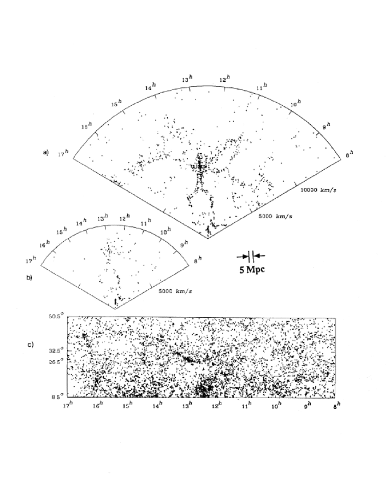
Figure 3: A slice of the three dimensional galaxy distribution (old CfA1 catalog (a) and new CfA catalog (b)) compared with the corresponding (c) angular distribution (the portion between $26.5^{\circ}$ and $32.5^{\circ}$) - from the de Lapparent et al.1988. Note that the angular distribution appears relatively homogeneous while the real three distribution in space is much more irregular. In particular this picture points out the so-called Great Wall which extends over the entire sample (at least $170h^{-1}Mpc$). We also show the size of the galaxy ”correlation-length” ($r_{0}=5h^{-1}Mpc$) derived from the standard analysis. The more general analysis we discuss here implies instead that an eventual correlation length should be larger than any observable structure, i.e. $\gg 170h^{-1}Mpc$ and that the present data show well defined fractal properties up to the sample limits.

Assuming that this smoothness corresponds to a real homogeneity in 3-d space and estimating the characteristic depth of the angular catalog from the magnitudes, ”a characteristic length” $r_{0}=5h^{-1}Mpc$ has been measured [3]. The idea was that beyond such a distance the 3-d galaxy distribution would become about homogeneous and it could be well approximated by a constant galaxy density. This value, apart from the eventual dark matter, is the one to use into Einstein equations to derive the Friedmann metric and the other usual concepts.

Later on, the measurements of the galactic redshifts, plus the Hubble law, provided also the absolute distances and could identify the position of galaxies in space. However, the 3-d galaxy distributions turned out to be much more irregular with respect to their angular projections and unveiled large structures and large voids, as shown in the upper part of Fig.3. At first these irregular structures appeared to be in contradiction with the picture derived from the angular catalogs and, as we discuss in what follows, they really are. However, in 1983, a correlation analysis of the 3-d distribution CfA1 catalog [17] was performed by Davis & Peebles [18] and the result was again that the correlation length was $r_{0}=5h^{-1}Mpc$ as for the angular catalogs. This seemed to resolve the puzzle, because it was interpreted as if a relatively small correlation length can be consistent with the observation of large structures. This value for $r_{0}$ has not been seriously questioned, even after the observation of huge structures, like the Galaxy Great Wall, that extend up to $\sim 170h^{-1}Mpc$ or more.

The usual correlation analysis is performed by estimating at which distance ($r_{0}$) the density fluctuations are comparable to the average density in the sample ($\xi(r)=\langle n(0)n(r)\rangle/\langle n\rangle^{2}-1$; $\xi(r_{0})\equiv 1$). Now it’s commonly accepted that there are fractal correlations at least at small scales [19] (see also [20]). The important physical question is therefore to identify the distance $\lambda_{0}$ at which, possibly, the fractal distribution has a crossover into a homogeneous one. The first question is whether there is, or not, such a crossover. This is the real correlation length, beyond which the distribution can be approximated by an average density. The problem is therefore to understand the relation between $r_{0}$ and $\lambda_{0}$: are they the same, or closely related, or do they correspond to different properties? This is, actually, a subtle point. In fact, if the galaxy distribution becomes really homogeneous at a scale $\lambda_{0}$ within the sample in question, then the value of $r_{0}$ is related to the real correlation properties of the distribution and one has $r_{0}\simeq\lambda_{0}/2$. If, on the other hand, the fractal correlations extend up to the sample limits, then the resulting value of $r_{0}$ has nothing to do with the real properties of galaxy distribution, but it is fixed just by the size of the sample [2].

New Perspective: Given this situation of ambiguity in relation with the real meaning of $r_{0}$, it is clear that the usual study of correlation in terms of the function $\xi(r)$ is not an appropriate method to clarify these basic questions. The essential problem is that, by using the function $\xi(r)$, one defines the amplitude of the density fluctuations by normalizing them to the average density of the sample in question. This implies that the observed density should be the real one and it should not depend on the given sample or on its size, apart from Poisson fluctuations. However, if the distribution shows long range (fractal) correlations, this approach becomes meaningless. For example, if one studies a fractal distribution using the concept $\xi(r)$ as defined previously, a characteristic length $r_{0}$ can be identified, but this is clearly an artifact because the structure is characterized exactly by the absence of any defined length [2]. It is important to stress that the so-called correlation length $r_{0}$ is just one of the statistical quantities used by the standard approach, which are not suitable to describe irregular (scale-invariant) distributions.

The appropriate analysis of correlations should, therefore, be performed using methods that can check homogeneity or fractal properties without assuming a priori either one. The simplest method to do this is to look directly at the conditional density $\Gamma(r)\sim\langle n(0)n(r)\rangle$, without normalizing it to the average. There are several other methods that we discuss in what follows. This is not all however, because one has also to be careful not to make hidden assumptions of homogeneity in the specific procedure to evaluate these correlations. For example, if a galaxy is close to the boundary of the sample, it is possible that the sphere of radius $r$ around it, where the conditional density is computed, may lie in part outside the sample boundary. In this case the usual procedure is to use weighting schemes of various types to include also these points in the statistics. In this way, one implicitly assumes that the fraction of sphere contained in the sample is sufficient to estimate the properties of the full sphere. This implies that the properties of a small volume are assumed to be the same as for a larger volume (the full sphere). This is a hidden assumption of homogeneity that should be avoided by including only the properties of those points for which a surrounding sphere of radius $r$ is fully included in the sample. These procedures are fully standard in modern Statistical Mechanics and a detailed description can be found in [2, 20] (Sec.2. and Sec.3). This means that the statistical validity of a sample is limited to the radius of the largest sphere that can be contained in the sample. We call this distance $R_{eff}$ and it should not be confused with the sample depth $R_{s}$, which can be in general much larger, depending on the survey geometry.

In 1988, we reanalyzed the CfA1 catalog [21]. The result was that the catalog has statistical validity up to $R_{eff}=20h^{-1}Mpc$ and, up to this length, it shows well defined fractal correlations with a value of the fractal dimension $D\approx 1.5$. This shows therefore that the ”correlation length” $r_{0}=5h^{-1}Mpc$ derived by [18], was a spurious result due to an inappropriate method of analysis and it has nothing to do with the real correlation properties of the system. A similar new analysis of the Abell cluster catalog also showed fractal properties up to $R_{eff}=80h^{-1}Mpc$, so that also the cluster ”correlation length” $r_{0}^{c}=25h^{-1}Mpc$ [22] should be considered as spurious. One consequence of these results was that the so called galaxy-cluster mismatch could be automatically eliminated by the appropriate analysis. Also other properties like $\delta N/N$, directly related to $r_{0}$, suffer from the same consistency problems because the lack of a reference value [9].

This situation led to a rather controversial debate in the field [19, 20]. In the meantime many more data became available and we decided to perform a complete analysis of all the data for galaxies and clusters. In what follows we report our main results.

1.2 Organization of the paper

Fractal Geometry provides a quantitative mathematical framework for the analysis and the characterization of irregular non analytic structures, as well as regular and homogeneous ones. We introduce in Sec.2 the main properties and concepts of fractal geometry which we use in the analyses presented in this work. In particular, we stress the conceptual consequence of the lack of any reference value, like the average density, in the case of self-similar structure and the consequent shift of the theoretical investigation from ”amplitudes” towards ”exponents”. The properties of the (average) conditional density are discussed. Such a quantity is the most important statistical tool that we use for the characterization of the correlation properties of galaxies and clusters.

The correlation analysis for various galaxy and cluster redshift surveys is presented in Sec.3, together with an broad and detailed discussion of the basic techniques that we employ. Moreover, we present several tests on the treatment of the boundary conditions, and on the stability of the correlation analysis versus eventual systematic and random errors that can affect the real data. Finally, we clarify the luminosity segregation effect, as well as the galaxy cluster mismatch, showing that these concepts arise only from an inconsistent data analysis.

The determination of the power spectrum is discussed in Sec.4. We point out the conceptual difficulties of the standard analysis and we introduce a more general determination of the power spectrum, that can be useful for the characterization of the properties of self-similar irregular systems, as well as regular ones.

How many galaxies should contain a galaxy sample, in order to be statistically meaningful ? The discussion of this important question allows us, in Sec.5, to clarify the concept of fair sample and to derive a quantitative criteria to define the statistical validity of samples.

In Sec.6 we introduce and discuss another determination of the galaxy space density: the radial density. This quantity is determined from a single point, and allows one to reach very large distances especially in the case of narrow and deep surveys. The price to pay, however, is that this quantity is not an average one. Hence, it is subject to finite size and intrinsic fluctuations, that must be study in great detail, in order to interpret correctly the experimental data. In particular the nature of intrinsic fluctuations which are inherent to fractal sets, is qualitatively different from the poissonian one. In this section, we summarize of the different determinations of the space density, i.e. by the conditional density and the radial density. The results of the correlation analysis in the various available redshift surveys are shown to be compatible with each other. In such a way we may present the full correlation analysis in the range $0.5\div 1000h^{-1}Mpc$. The result is that galaxy properties are compatible in the different catalogs, and there are fractal correlations with dimension $D=2.0\pm 0.2$ up to the deepest scale observed for visible matter.

At the light of the interpretation of the radial density behavior, we discuss in Sec. 7 the analysis of the number counts as a function of the apparent flux (or magnitude). The counts of various astrophysical objects are usually characterized by a spurious regime at bright fluxes, that seems to be nearly Euclidean. At faint apparent fluxes (or magnitudes) the number counts deviates from the Euclidean behavior, having a well defined exponent. The crucial point in this case is that the counts are determined by the Earth, without performing an average over different observers. This leads to finite size spurious fluctuations, as well as intrinsic ones which are not smoothed out by averaging, which dramatically affect the behavior at small scale, i.e. at the bright end of the number counts. On the other hand at faint fluxes, as the space volume involved is large enough, it is possible to obtain the genuine scaling behavior without performing averages. Our new interpretation shows that the counts of different astrophysical objects, such as galaxies in the different spectral bands, X-ray sources, Radio-Galaxies, Quasars are all compatible with a scale-invariant distribution with dimension $D\approx 2$ up to the faint end of the counts, that is to say the deepest scales ever investigated for visible matter (i.e., $m\sim 29$ in the $B$ band for optical galaxies). Finally we clarify the problems of angular correlations, namely the uniformity and isotropic nature of the angular projection of fractal structures, and the scaling of the amplitude of the angular correlation function.

In Sec.8 we consider, by a quantitative analysis, an important observational fact: galaxy positions and luminosities are strongly correlated. This fact has lead to various morphological interpretation of the distribution of galaxies with different luminosity. In this section, we present the multifractal analysis of galaxy distribution. Such an analysis allows us to consider the correlation between the space and luminosity distributions within a quantitative mathematical framework, and to unify these two distributions. Moreover, we clarify the segregation of luminous galaxies in the core of clusters and fainter ones in the field, in terms of multifractals. The multifractality of matter distribution should therefore claim a central stage in theoretical investigations.

Finally in Sec.9 we present our main conclusions. We stress the paradoxical situation due to the coexistence of the fractal distribution of visible matter and the strictly linear Hubble law at the same scales. In fact, in the standard scenario of the Friedmann models, the Hubble law is a consequence of the assumption of homogeneity of matter distribution. We examine various possible solutions of such a problem with particular emphasis on the role of the so-called dark matter. Moreover we discuss the theoretical implications and change of perspective implied by our results. At the end of this section we briefly present our predictions for the forthcoming redshift surveys like CfA2, 2dF, and SLOAN.

In the Appendix we report all the details of the catalogs analyzed: CfA1, SSRS1, Perseus-Pisces, IRAS $2Jy$, IRAS $1.2Jy$, Las Campanas Redshift Survey, the ESO Slice Project, and the Stromlo-APM redshift survey for galaxies (we have considered and discussed also the SSRS2 and CfA2 redshift surveys, which are not yet published) and Abell and ACO for galaxy clusters.

2 Statistical methods and correlation properties for galaxy distributions

We have discussed in a series of papers [1, 21, 2, 9, 23, 24] the conceptual problems of the standard correlation analysis and we have introduced the correct correlation analysis that should be applied for the characterization of the statistical properties of irregular as well as regular distributions. Here we briefly review the main results and we introduce the basic concepts of fractal geometry.

2.1 Usual analysis, conceptual problems and correlation lengths

In the following description the galaxy is treated as a point (while in Sec.8 we consider whole mass distribution). In this case the statistical analysis is performed only on the number density, neglecting the masses of galaxies,

$$n(\vec{r})=\sum_{i=1}^{N}\delta(\vec{r}-\vec{r}_{i})\,.$$ (1)

The standard statistical analysis considers only the number density (Eq.1) and it consists in the computation of the so-called $\xi(r)$ correlation function defined as [25]

$$\xi(r)=\frac{\langle n(\vec{r}_{*})n(\vec{r}_{*}+\vec{r})\rangle}{\langle n\rangle^{2}}-1$$ (2)

where the average is defined as

$$\langle\cdot\cdot\cdot\rangle=\frac{1}{V}\int_{V}(\cdot\cdot\cdot)d\vec{r}_{*}$$ (3)

and

$$\langle n\rangle=\frac{N}{V}$$ (4)

is the average density of galaxies in the sample ($V$ is the sample volume and $N$ is the number of galaxies contained in that volume). In the computation of $\xi(r)$ (Eq.2) it is performed the angular average over all the possible directions, and only the radial dependence is considered. From the very definition of $\xi(r)$ it follows that [2]

$$\int_{V}\xi(r)dr=0\;.$$ (5)

This means that if $\xi(r)$ is positive for some range of values of $r$, then there must be other ranges in which it is negative, in view of its definition as a measure of fluctuations from the average. $\xi(r)$ is an appropriate function to characterize correlations for systems in which the average density (Eq.4) is a well defined intrinsic property, as for example in liquids. In this case the average density $\langle n\rangle$ is a well defined quantity beyond a certain scale (say several times the mean interparticle separation), and the definition of $\xi(r)$ is meaningful. In fact, if the system shows correlations then $\langle n(\vec{r}_{*})n(\vec{r}_{*}+\vec{r})\rangle\gg\langle n\rangle^{2}$ so that $\xi(r)\neq 0$, while if there are no correlations $\xi(r)=0$. The distance $r_{0}$ defined as $\xi(r_{0})=1$, separates a correlated regime characterized by large fluctuations, from a regime of negligible fluctuations.

In the case of irregular systems, characterized by large structures and voids, the average density is not a well defined property, and the $\xi(r)$ analysis gives rise to spurious results. In other words the homogeneity assumption used in the $\xi(r)$ analysis must be seriously questioned.

2.1.1 Three dimensional galaxy and cluster distributions

As we have already mentioned in the previous section, the usual statistical analysis of galaxy correlation is performed by measuring the $\xi(r)$ function in three dimensional samples. In the past twenty years, this kind of analysis has been performed for galaxy and cluster distributions (Sec.3; for a detailed discussion; we refer to [3, 19, 26, 25] for a review of the state of the art in the field) and the results are quite similar. At small distances, the standard two point correlation function can be characterized by a power law behavior

$$\xi_{GG}(r)\sim A_{G}r^{-\gamma_{GG}}$$ (6)

where $\gamma_{GG}\approx 1.7$. The so-called correlation length $r_{0}$ is defined as $\xi(r)\equiv 1$, so that we have [25, 19]

$$r_{0}^{G}=A_{G}^{\frac{1}{\gamma_{GG}}}\approx 5h^{-1}Mpc\;.$$ (7)

At twice this distance the $\xi(r)$ function deviates from a power law behavior and becomes negative or zero (Fig.4).

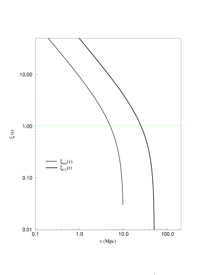
Figure 4: Standard analysis of galaxy $\xi_{GG}$ and cluster $\xi_{CC}$ distributions. The two functions show power law behavior with about the same exponent, but the one corresponding to cluster has a larger amplitude.

In the case of galaxy clusters, the volumes explored are larger than those of galaxy catalogs. However the behavior of the standard correlation function is found to be quite similar to that of galaxies, and, at small scales, it has been measured [22] that

$$\xi_{CC}(r)\sim A_{C}r^{-\gamma_{CC}}$$ (8)

where $\gamma_{CC}\approx 1.7$ as in the case of galaxies. The amplitude $A_{C}$ is larger than $A_{G}$, so that the cluster correlations length is

$$r_{0}^{C}=A_{C}^{\frac{1}{\gamma_{C}}}\approx 25h^{-1}Mpc\;.$$ (9)

The difference between galaxy and cluster correlation length is known as the ”galaxy - cluster mismatch”. Various interpretations in literature have been proposed in order to explain such a result. We show later that the self-similar behavior of galaxy and cluster distributions naturally resolve this apparent mismatch (Sec.3.2).

2.1.2 Angular distributions

The problem of the angular analysis consists of the reconstruction of the three dimensional properties of galaxy distribution from the knowledge of the angular coordinates and the apparent magnitude. This is a very complex problem (see also Sec.7 and Sec.8), and the standard analysis does not consider some conceptual and fundamental difficulties, which make very hard the deduction of the three dimensional properties from the angular information.

The standard method used to analyze angular catalogs, is based on the assumption that galaxies are correlated only at small distances. In such a way the effect of the large spatial inhomogeneities is not considered at all. Under this assumption, that is not supported by any experimental evidence, it is possible to derive the Limber equation [27, 28]. In practice, the angular analysis is performed by computing the two point correlation function

$$\omega(\theta)=\frac{\langle n(\theta_{0})n(\theta_{0}+\theta)\rangle}{\langle n\rangle}-1$$ (10)

that is the analogue of Eq.2 for the angular coordinates. The results of such an analysis are quite similar to the three dimensional ones. In particular, it has been obtained that, in the limit of small angles,

$$\omega(\theta)=\theta^{-\gamma+1}$$ (11)

with $\gamma\approx 1.7$. It is possible to show [25] that, in the Limber approximation (Eq.11), the angular correlation function corresponds to $\xi(r)\sim r^{-\gamma}$ for its three dimensional counterpart (in the case $\gamma>1$). The determination of the correlation length is more complex, and it requires a comparison of catalogs with different depth, i.e. with different apparent magnitude limit. Using the Limber equation and the assumption that the luminosity distribution is independent on the spatial one, it is possible to derive the following relation

$$\omega^{\prime}(\theta^{\prime}_{12}=(R_{s}/R_{s}^{\prime})\theta_{12})=(R_{s}/R_{s}^{\prime})\omega(\theta_{12})\;.$$ (12)

Such an equation links the depth of a certain catalog $R_{s}$ to that of another catalog $R_{s}^{\prime}$. In Fig.5

Figure 5: (a) Scaling test of the two point angular correlation function with sample depth (different apparent magnitude limit) in the APM angular catalog (from Maddox et al., 1990). In (b) it is shown the rescaling of the angular correlation function, by applying Eq.12, that holds for a homogeneous distribution. We refer to Sec.7 for a detailed discussion of such a test.

it is shown the dependence of the amplitude of $\omega(\theta)$ with sample depth. The fact that Eq.12 is found to be satisfied in real catalogs, has been interpreted as an evidence of homogenization [3]. The corresponding correlation length is quite similar to that found in the three dimensional catalogs, i.e. $r_{0}\approx 5h^{-1}Mpc$. However this kind of analysis suffers of the same problems of $\xi(r)$, and it is based on untested assumptions. In particular the main point is that it does not take into account the effects of spatial inhomogeneities.

2.2 Large structures, long range correlations and fractal properties

Fractals are simple but subtle. In this section we provide a brief description of their essential properties. This description is intended to illustrate the consequences of the properties of self-similarity so that, if this property is actually present in the experimental data, we are able to detect it correctly; on the contrary, if the data were not consistent with the fractal properties, we have to know well the properties of fractals in order to eventually conclude that observations are actually in contrast with them.

A basic element of fractal structures is that if one magnifies a small portion of them, this reveals a complexity comparable to that of the entire structure. This is geometric self-similarity and it has deep implications about the non-analyticity of these structures. In fact, analyticity or regularity implies that at some small scale the profile becomes smooth and one can define a unique tangent. Clearly this is impossible in a self-similar structure because at any small scale a new structure appears and the structure is never smooth. Self-similar structures are therefore intrinsically irregular at all scales and this is why many familiar phenomena have remained at the margins of scientific investigation. The usual mathematical concepts in Physics are mostly based on analytical functions and, in this perspective, irregularities are seen as imperfections. Fractal geometry changes completely this perspective by focusing exactly on these intrinsic irregularities and it allows us to characterize them in a quantitative mathematical way.

2.2.1 The ”Mass-length” relation

A fractal is a system in which more and more structures appear at smaller and smaller scales and the structures at small scales are similar to the one at large scales. In Fig.6, we show an elementary (deterministic) fractal distribution of points in space whose construction is trivial. Starting from a point occupied by an object, we count how many objects are present within a volume characterized by a certain length scale, in order to establish a generalized ”mass-length” relation from which one can define the fractal dimension.

Figure 6: A simple example of a deterministic fractal in the two dimensional Euclidean space. The same structure repeats at different scales in a self-similar way.

Suppose that, in the structure of Fig.6, we can find $N_{0}$ objects in a volume of size $\>r_{0}$. If we consider a larger volume of size $\>r_{1}=k\cdot r_{0}$, we find $\>N_{1}={\tilde{k}}\cdot N_{0}$ objects. In a self-similar structure, the parameters $\>k$ and $\>{\tilde{k}}$ are the same also for other changes of scale. So, in general, in a structure of size $\>r_{n}=k^{n}\cdot r_{0}$, we have $\>N_{n}={\tilde{k}^{n}}\cdot N_{0}$ objects. We can then write a (average) relation between $\>N$ (”mass”) and $\>r$ (”length”) of type

$$N(r)=B\cdot r^{D}$$ (13)

where $D$ is the fractal dimension

$$D=\frac{log{\tilde{k}}}{logk}$$ (14)

and depends on the rescaling factors $\>k$ and $\>{\tilde{k}}$. The prefactor $\>B$ is instead related to the lower cut-offs $\>N_{0}$ and $\>r_{0}$ of the structure

$$B=\frac{N_{0}}{r_{0}^{D}}\;.$$ (15)

It should be noted that Eq.13 corresponds to a smooth convolution of a strongly fluctuating function as evident in Fig.6. Therefore a fractal structure is always connected with large fluctuations and clustering at all scales.

From Eq.13 we can readily compute the average density $\><n>$ for a sample of radius $\>R_{s}$ which contains a portion of the fractal structure. The sample volume is assumed to be a sphere ($\>V(R_{s})=(4/3)\pi R_{s}^{3}$) and therefore

$$<n>=\frac{N(R_{s})}{V(R_{s})}=\frac{3}{4\pi}BR_{s}^{-(3-D)}\;.$$ (16)

From Eq.16 it follows that the average density is not a meaningful concept in a fractal because it depends explicitly on the sample size $\>R_{s}$. Moreover for $\>R_{s}\rightarrow\infty$ the average density $\><n>\rightarrow 0$: this implies that a fractal structure is asymptotically dominated by voids. Therefore the average density $\><n>$ is not a well defined quantity: the amplitude of this function essentially refers to the unit of measures given by the lower cut-offs but it has no particular physical meaning. We can also define the conditional density from any point occupied as

$$\Gamma(r)=S^{-1}\frac{dN(r)}{dr}=\frac{D}{4\pi}Br^{-(3-D)}$$ (17)

where $\>S(r)$ is the area of a spherical shell of radius $\>r$. The conditional average density, as given by Eq.17, is well defined in terms of its exponent, the fractal dimension. Usually the exponent that defines the decay of the conditional density $\>(3-D)$ is called the codimension and it corresponds to the exponent $\>\gamma$ of the galaxy distribution. In Fig.7(b) we show a stochastic fractal (generated by the random-$\>\beta$-model algorithm [30] in the two dimensional Euclidean space - see Sec.7.5.1) constructed with a probabilistic algorithm with a well defined fractal dimension $\>D=1.2$.

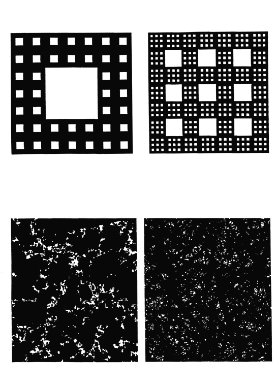
Figure 7: (a) Two deterministic fractals of identical fractal dimension and sharply distinct form. (b) Two random fractals of identical and different lacunarity. These structures are obtained by the random $\beta$ model algorithm, with different shaped voids (lacunarity) (Courtesy of B. Mandelbrot).

2.2.2 Power laws, self-similarity and non-analyticity

From Fig.6 the geometrical self-similarity is evident in the construction, while in Fig.7, only a detailed analysis can show the self-similarity of the structure. From a mathematical point of view self-similarity implies that a rescaling of the length by a factor $\>b$

$$r\rightarrow r^{\prime}=br$$ (18)

leaves the correlation function unchanged apart from a rescaling that depends on $\>b$ but not on the variable $\>r$. This leads to the functional relation

$$\Gamma(r^{\prime})=\Gamma(b\cdot r)=A(b)\cdot\Gamma(r)$$ (19)

which is clearly satisfied by a power law with any exponent ($A(b)$ is a prefactor depending on $b$ only). In fact, for

$$\Gamma(r)=\Gamma_{0}r^{\alpha}$$ (20)

we have

$$\Gamma(r^{\prime})=\Gamma_{0}(br)^{\alpha}=(b)^{\alpha}\Gamma(r)\;.$$ (21)

Note that Eq.19 does not hold, for example, for an exponential function

$$\Gamma(r)=\Gamma_{0}e^{-r/r_{0}}\;.$$ (22)

This reflects the fact that power laws do not possess a characteristic length, while for the exponential decay, $\>r_{0}$ is a characteristic length. Note that the characteristic length has nothing to do with the prefactor of the exponential and it is not defined by the condition $\>\Gamma(r_{0})=1$, but from the intrinsic behavior of the function. This brings us to a common misconception that sometimes occurs in the discussion of galaxy correlations. Even for a perfect power law as Eq.20, one might use the condition $\>\Gamma(r_{0})=1$ to derive a ”characteristic length”:

$$r_{0}=\Gamma_{0}^{-1/\alpha}\;.$$ (23)

This however is completely meaningless because the power law refers to a fractal structure constructed as self-similar and, therefore, without a characteristic length. In Eq.23, the value of $\>r_{0}$ is just related to the power law amplitude that, as we have already pointed out, has no physical meaning. The point is that the value 1 used in the relation $\>\Gamma(r_{0})=1$, is not particular in any way, so one may have used, as well, the condition $\>\Gamma(r_{0})=10^{10}$ or $\>\Gamma(r_{0})=10^{-10}$ to obtain other lengths. This is the subtle point of self-similarity; there is no reference value (like the average density) with respect to which one can define what is big or small.

We have discussed how self-similarity implies power laws: we consider now the inverse problem, namely, whether a power law implies self-similarity. This point allows us to stress the non-analytic nature of fractal structures. This question can be examined with a simple example. We consider a density $\rho(r)$ that behaves, in three dimensions, as

$$\rho(r)=\frac{1}{r}.$$ (24)

One can argue that the mass-length relation is given by

$$N(<r)\approx\int_{0}^{R}\rho(r)r^{2}dr\approx R^{2}$$ (25)

and therefore interpret the exponent $2$ as the fractal dimension of this distribution. This not correct, because Eq.25 holds only for one specific origin ($r=0$), while for a fractal it should hold for any origin. For any other origin one obtains

$$N(<r)\approx\int_{0}^{R}\rho(\vec{r}_{0}+\vec{r})d\vec{r}.$$ (26)

For $|\vec{r}_{0}|>R$ we can approximate the density as (Fig.2 upper part)

$$\rho(\vec{r}_{0}+\vec{r})\approx\rho(\vec{r}_{0})=\rho_{0}$$ (27)

and therefore

$$N(<r)\approx\int_{0}^{R}\rho_{0}r^{2}dr\approx\rho_{0}R^{3}.$$ (28)

This gives the standard dimension of the embedding space that shows we are dealing with a smooth (except for the point $\vec{r}=0$), nonfractal distribution. For homogeneous fractals, one should find the same nontrivial exponent $D<3$, no matter which lower integration limit is considered. The power law is non-analytic at the origin but this actually refers to each occupied point of the system. Thus the system is globally non-analytic because each point corresponds to a singularity.

2.2.3 Lacunarity and voids distribution

So far we have quantified fractal structures by their dimension. That this is not a sufficient characterization is illustrated in Fig.7. We illustrate the construction of two Cantor sets (one deterministic and one stochastic) with the same fractal dimension $D$ but with different morphological properties. In order to distinguish such sets, Mandelbrot [14] has introduced the concept of lacunarity $F$ as

$$Nr(\lambda>\Lambda)=F\Lambda^{-D}$$ (29)

where $Nr(\lambda>\Lambda)$ is the number of voids with a size $\lambda>\Lambda$. The scaling behavior of $Nr(\lambda)$ is the same for both Cantor sets. However the lacunarity $F$, i.e. the prefactor of the distribution, takes different values for the two Cantor sets.

In order to define lacunarity for random fractals we need a probabilistic form of Eq.29. This can be done by introducing $P(\lambda)$, which is the conditional probability that, given a box of size $\epsilon$ containing points of the set, this box is neighbored by a void of size $\lambda>\Lambda$. Lacunarity is defined as the prefactor of the void distribution

$$P(\lambda>\Lambda)=F\Lambda^{-D}\;.$$ (30)

It is easy to show [31] that in the case of deterministic fractals this definition gives the same value of the lacunarity defined in Eq.29. Lacunarity plays a very important role in the characterization of voids distribution in the available galaxy catalogs [32] (Sec.6 and Sec.7).

2.2.4 Properties of orthogonal projection and intersections

We briefly present the properties of orthogonal projections and intersections of fractal structures. This discussion is useful in the interpretation of angular and one dimensional (pencil beams) catalogs (Sec.6 and Sec.7).

Orthogonal projections preserves sizes of objects. If an object of fractal dimension $D$, embedded in a space of dimension $d=3$, is projected on a plane (of dimension $d^{\prime}=2$) it is possible to show that the projection has dimension $D^{\prime}$ such that [33, 2]

$$D^{\prime}=D\;\;\mbox{if}\;\;D<d^{\prime}=2\;;\;D^{\prime}=d^{\prime}\;\;\mbox{if}\;\;D>d^{\prime}=2\;.$$ (31)

This explains, for example, why clouds which have fractal dimension $D\approx 2.5$, give rise to a compact shadow of dimension $D^{\prime}=2$. The angular projection represents a more complex problem due to the mix of very different length scales (Sec.7 ). Nevertheless the theorem given by Eq.31 can be extended to the case of angular projections in the limit of small angles [34].

We discuss now a different but related problem: which are the properties of the structure that comes out from the intersection of a fractal with dimension $D$, embedded in the $d=3$ Euclidean space, with an object of dimension $D^{\prime}$ ? The last can be for example a line ($D^{\prime}=1$ - schematically a pencil beam survey), a plane ($D^{\prime}=2$) or a random distribution ($D^{\prime}=3$). It is possible to show [14, 2] that the law of codimension additivity gives for the dimension of the intersection

$$D_{I}=D+D^{\prime}-d$$ (32)

If $D_{I}\leq 0$, in the intersection it is not possible to recover any correlated signal [2]. Hence for example the intersection of a stochastic fractal with a random distribution has the same dimension $D_{I}=D$ of the original structure. Such a property is useful in the discussion of surveys in which a random sampling has been applied (Sec.3).

2.3 General properties of correlations

In this section we discuss how to perform the correct correlation analysis that can be applied to an irregular distribution as well as to a regular one. We start recalling the concept of correlation. If the presence of an object at the point $r_{1}$ influences the probability of finding another object at $r_{2}$, these two points are correlated. Therefore there is a correlation at $r$ if, on average

$$G(r)=\langle n(0)n(r)\rangle\neq\langle n\rangle$$ (33)

where we average on all occupied points chosen as origin. On the other hand, there is no correlation if

$$G(r)\approx\langle n\rangle^{2}.$$ (34)

The physically meaningful definition of $\lambda_{0}$ is therefore the length scale which separates correlated regimes from uncorrelated ones.

In practice, it is useful to normalize the CF to the size of the sample analyzed. Then we use, following [2, 35] the average conditional density defined as

$$\Gamma(r)=\frac{<n(r)n(0)>}{<n>}=\frac{G(r)}{<n>}$$ (35)

where $\><n>$ is the average density of the sample. We stress that this normalization does not introduce any bias even if the average density is sample-depth dependent, as in the case of fractal distributions, because it represents only an overall normalizing factor. In order to compare results from different catalogs it is however more useful to use $\Gamma(r)$, in which the size of a catalog only appears via the combination $N^{-1}\sum_{i=1}^{N}$, so that a larger sample volume only enlarges the statistical sample over which averages are taken. $G(r)$ instead has an amplitude that is an explicit function of the sample’s size scale. $\Gamma(r)$ (Eq.35) can be computed by the following expression

$$\Gamma(r)=\frac{1}{N}\sum_{i=1}^{N}\frac{1}{4\pi r^{2}\Delta r}\int_{r}^{r+\Delta r}n(\vec{r}_{i}+\vec{r^{\prime}})d\vec{r^{\prime}}=\frac{BD}{4\pi}r^{D-3}$$ (36)

where the last equality follows from Eq.17. This function measures the average density at distance $\>\vec{r}$ from an occupied point at $\vec{r_{i}}$ and it is called the conditional density [2]. If the distribution is fractal up to a certain distance $\lambda_{0}$, and then it becomes homogeneous, we have that $\Gamma(r)$ has a power law decaying with distance up to $\lambda_{0}$, and then it flattens towards a constant value. Hence by studying the behavior of $\Gamma(r)$ it is possible to detect the eventual scale-invariant properties of the sample. Instead the information given by the $\xi(r)$ is biased by the a priori (untested) assumption of homogeneity.

It is also very useful to use the integrated conditional density

$$\Gamma^{*}(r)=\frac{3}{4\pi r^{3}}\int_{0}^{r}4\pi r^{\prime 2}\Gamma(r^{\prime})dr^{\prime}=\frac{3B}{4\pi}r^{D-3}$$ (37)

This function produces an artificial smoothing of rapidly varying fluctuations, but it correctly reproduces global properties [2].

For a fractal structure, $\Gamma(r)$ has a power law behavior and the integrated conditional density is

$$\Gamma^{*}(r)=\frac{3}{D}\Gamma(r).$$ (38)

For an homogeneous distribution ($D=3$) these two functions are exactly the same and equal to the average density.

2.3.1 The $\xi(r)$ correlation function for a fractal

Pietronero and collaborators [1, 21, 2] have clarified some crucial points of the standard correlations analysis, and in particular they have discussed the physical meaning of the so-called ”correlation length” $\>r_{0}$ found with the standard approach [25, 18] and defined by the relation:

$$\xi(r_{0})\equiv 1$$ (39)

where

$$\xi(r)=\frac{<n(\vec{r_{0}})n(\vec{r_{0}}+\vec{r})>}{<n>^{2}}-1$$ (40)

is the two point correlation function used in the standard analysis. The basic point in the present discussion, is that the mean density, $<n>$, used in the normalization of $\>\xi(r)$, is not a well defined quantity in the case of self-similar distribution and it is a direct function of the sample size. Hence only in the case that homogeneity has been reached well within the sample limits the $\>\xi(r)$-analysis is meaningful, otherwise the a priori assumption of homogeneity is incorrect and characteristic lengths, like $\>r_{0}$, became spurious.

For example from Eq.16 and Eq.36 the expression of the $\>\xi(r)$ in the case of fractal distributions is [2]:

$$\xi(r)=\frac{3-\gamma}{3}\left(\frac{r}{R_{s}}\right)^{-\gamma}-1$$ (41)

where $\>R_{s}$ is the depth of the spherical volume where one computes the average density from Eq.16. From Eq.41 it follows that

i.) the so-called correlation length $\>r_{0}$ (defined as $\>\xi(r_{0})\equiv 1$) is a linear function of the sample size $\>R_{s}$

$$r_{0}=\left(\frac{3-\gamma}{6}\right)^{\frac{1}{\gamma}}R_{s}$$ (42)

and hence it is a spurious quantity without physical meaning but it is simply related to the sample finite size (Fig.8).

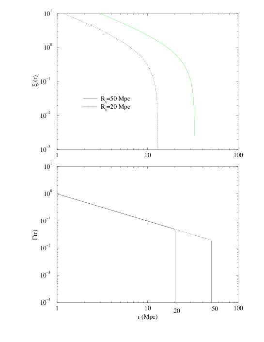
Figure 8: Upper part: $\xi(r)$ computed for a self-similar structure contained in a sample of radius $R_{s}=20Mpc$. If one computes such a quantity in a sample of radius $R_{s}^{\prime}=50Mpc$, one can see how inappropriate this function is in view of its explicit dependence on the sample size. Bottom part: It is shown the same exercise for $\Gamma(r)$. The amplitude and the slope of the conditional density perfectly matches the one obtained in the smaller sample.

ii.) $\>\xi(r)$ is power law only for

$$\left(\frac{3-\gamma}{3}\right)\left(\frac{r}{R_{s}}\right)^{-\gamma}\gg 1$$ (43)

hence for $r\ll r_{0}$: for larger distances there is a clear deviation from the power law behavior due to the definition of $\xi(r)$. This deviation, however, is just due to the size of the observational sample and does not correspond to any real change of the correlation properties. It is clear that if one estimates the $\xi(r)$ exponent at distances $r\mathrel{\hbox to0.0pt{\lower 3.0pt\hbox{$\mathchar 536\relax$}\hss}\raise 2.0pt\hbox{$\mathchar 316\relax$}}r_{0}$, one systematically obtains a higher value of the correlation exponent due to the break of $\xi(r)$ in the log-log plot. For example we can compute the $\xi(r)$ function for a fractal with dimension $D=2$ (i.e $\gamma=1$) in two samples of different depths: the first has $R_{s}=20Mpc$ while the second has $R_{s}=100Mpc$ (Fig.9).

Figure 9: The $\xi(r)$ function computed for a fractal with dimension $D=2$ ($\gamma=3-D=1$) in two samples of different depth $R_{s}$. In the first case $R_{s}=20Mpc$ one obtains an higher value for the correlation exponent $\gamma=1.7$ because one performs the fit in the region of length scales $r\sim r_{0}$. In the second case the power law behavior of $\xi(r)$ is more extended ($R_{s}=100Mpc$) and by evaluating the exponent in the region $r\ll r_{0}$ one obtains the correct value for the correlation exponent $\gamma=1$.

In the first case one fits the $\xi(r)$ with a power law function in the region of length scales $r\sim r_{0}$ and in such a way one obtains a higher value for the correlation exponent, i.e. $\gamma=1.7$. In the second case, as the power law behavior is more extended, one can measure the correlation exponent in the range $r\ll r_{0}$ and doing so, one obtains the correct value for $\gamma=1$. For the same reason one obtains a larger value of $\gamma$ by the angular correlation $\omega(\theta)$ analysis.

The analysis performed by $\xi(r)$ is therefore mathematically inconsistent, if a clear cut-off towards homogeneity has not been reached, because it gives an information that is not related to the real physical features of the distribution in the sample, but to the size of the sample itself.

2.4 Problems of treatment of boundary conditions and sample size effects

Given a certain spherical sample with solid angle $\Omega$ and depth $R_{s}$, it is important to define which is the maximum distance up to which it is possible to compute the correlation function ($\Gamma(r)$ or $\xi(r)$). As discussed in [2], we limit our analysis to an effective depth $R_{eff}$ that is of the order of the radius of the maximum sphere fully contained in the sample volume (Fig.10).

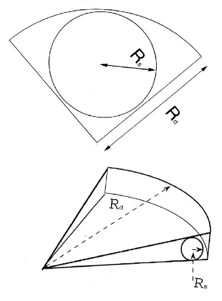
Figure 10: Upper part: A typical cone diagram for a wide angle galaxy catalog (e.g. CfA, SSRS, Perseus-Pisces). The depth is $R_{d}$. The effective depth is $R_{eff}$ and it corresponds to the radius of the maximum sphere fully contained in the sample volume ($R_{eff}\mathrel{\hbox to0.0pt{\lower 3.0pt\hbox{$\mathchar 536\relax$}\hss}\raise 2.0pt\hbox{$\mathchar 316\relax$}}R_{s}$). Bottom part: A typical cone diagram for a narrow angle galaxy catalog (e.g. LCRS, ESP). In this case $R_{eff}<<R_{d}$.

For example for a catalog with the limits in right ascension ($\alpha_{1}\leq\alpha\leq\alpha_{2}$) and declination ($\delta_{1}\leq\delta\leq\delta_{2}$) we have that

$$R_{eff}=\frac{R_{s}sin(\delta\theta/2)}{1+sin(\delta\theta/2)}$$ (44)

where $\delta\theta=min(\alpha_{2}-\alpha_{1},\delta_{2}-\delta_{1})$. In such a way we do not consider in the statistics the points for which a sphere of radius r is not fully included within the sample boundaries. Hence we do not make use of any weighting scheme with the advantage of not making any assumption in the treatment of the boundaries conditions. For this reason we have a smaller number of points and we stop our analysis at a smaller depth than that of other authors.

The reason why $\Gamma(r)$ (or $\xi(r)$) cannot be computed for $r>R_{eff}$ is essentially the following. When one evaluates the correlation function (or power spectrum) beyond $R_{eff}$, then one makes explicit assumptions on what lies beyond the sample’s boundary. In fact, even in absence of corrections for selection effects, one is forced to consider incomplete shells calculating $\Gamma(r)$ for $r>R_{eff}$, thereby implicitly assuming that what one does not find in the part of the shell not included in the sample is equal to what is inside (or other similar weighting schemes). In other words, the standard calculation introduces a spurious homogenization which we are trying to remove.

If one could reproduce via an analysis that uses weighting schemes, the correct properties of the distribution under analysis, it would be not necessary to produce wide angle survey, and from a single pencil beam deep survey it would be possible to study the entire matter distribution up to very deep scales. It is evident that this could not be the case. By the way, we have done a test on the homogenization effects of weighting schemes on artificial distributions as well as on real catalogs (Sec.3.4), finding that the flattening of the conditional density is indeed introduced owing to the weighting, and does not correspond to any real feature in the galaxy distribution.

The conditional density $\Gamma(r)$ (Eq.36) measures the density in a shell of thickness $\Delta r$ at distance $r$ from an occupied point, and then it is averaged over all the points of the sample. In practice, we have three possibilities for $\Gamma(r)$: i) $D=3$: in this case this function is simply a constant. ii) $0<D<3$ In this case the conditional density has a power law decay with exponent $-\gamma=D-3$. Finally iii) $D=0$: this is the limiting case in which there are no further points in the sample except the observer. In such a situation we have that $\Gamma(r)$ behaves as $1/r^{3}$, i.e. as the 3-d volume. Suppose now, for simplicity, we have a spherical sample of volume $V$ in which there are $N$ points, and we want to measure the conditional density. The maximum depth is limited by the radius of the sample (as previously discussed), while the minimum distance depends on the number of points contained in the volume. For a Poisson distribution the mean average distance between near neighbor is of the order $\ell\sim(V/N)^{\frac{1}{3}}$. Of course, such a relation does not express an useful quantity in the case of a fractal distribution, as well as the average density, while the meaningful measure is the average minimum distance between neighbor galaxies $\ell_{min}$, that is related to the lower cut-off of the distribution. If we measure the conditional density at distances $r\ll\ell_{min}$, we are affected by a finite size effect. In fact, due the depletion of points at these distances we underestimate the real conditional density finding an higher value for the correlation exponent (and hence a lower value for the fractal dimension). In the limiting case at distances $r<<\ell_{min}$, we can find almost no points and the slope is $\gamma=-3$ ($D=0$). In general, when one measures $\Gamma(r)$ at distances that correspond to a fraction of $\ell_{min}$, one finds systematically an higher value of the conditional density exponent. Such a trend is completely spurious and due to the depletion of points at such distances.

For example in a real survey, in order to check this effect, one should measure $\Gamma(r)$ in samples with different values of $\ell_{min}$ (Sec.3). In general we find that the sparser samples exhibit a change of slope, towards an higher value of the correlation exponent, at small distances. For the samples for which $\ell_{min}$ is quite small, the change of slope at small distances is not found. In general for a typical sample of galaxies (Sec.3 and the Appendix) $\ell_{min}\sim 1\div 6h^{-1}Mpc$, so that the behavior of $\Gamma(r)$ at distances of some Megaparsec is generally affected by this finite size effect. A way to reduce this effect is to chooses properly the thickness $\Delta r$ of the shell in which the conditional density is computed: this means that at small distances $\Delta r$ must be of the order of $\ell_{min}$ and not smaller than this value. In general we have found that best way to optimize this estimate is to choose logarithm interval for $\Delta r$, as a function of the scale in which the conditional density is computed.

2.5 Amplitude of fluctuations: linear and non-linear dynamics

Another argument often mentioned in the discussion of large-scale structures, is that it is true that larger samples show larger structures but their amplitudes are smaller and the value of $\>\delta N/N$ tends to zero at the limits of the sample [3]; therefore one expects that just going a bit further, homogeneity may finally be observed. Apart from the fact that this expectation has been systematically disproved, the argument is conceptually wrong for the same reasons of the previous discussion. In fact, we can consider a portion of a fractal structure of size $\>R_{s}$ and study the behavior of $\>\delta N/N$. The average density $\>N$ is just given by Eq.16 while the overdensity $\>\delta N$, as a function of the size $\>r$ ($\>r\leq R_{s}$) of a given in structure is:

$$\delta N=\frac{N(r)}{V(r)}-<n>=\frac{3}{4\pi}B(r^{-(3-D)}-R_{s}^{-(3-D)})\;.$$ (45)

We have therefore

$$\frac{\delta N}{N}=\left(\frac{r}{R_{s}}\right)^{-(3-D)}-1\;.$$ (46)

Clearly for structures that approach the size of the sample, the value of $\>\delta N/N$ becomes very small and eventually becomes zero at $\>r=R_{s}$ as shown in Fig.11.

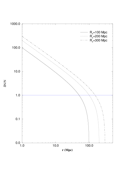
Figure 11: Behavior of $\>\delta N/N$ as a function of the size $r$ in a portion of a fractal structure for various depths of the sample: $\>R_{s}=100,200,300Mpc$. The average density is computed over the whole sample of radius $\>R_{s}$. The fact that $\>\delta N/N$ approaches to zero does not mean that the fluctuations are small and a homogeneous distribution has been reached. The distance at which $\>\delta N/N=1$ scales with sample depth and it has no physical meaning. In the case of a fractal distribution the normalization factor, i.e. the average density, is not an intrinsic quantity.

This behavior, however, cannot be interpreted as a tendency towards homogeneity because again the exercise refers to a self-similar fractal by construction. Also in this case, the problems come from the fact that one defines an ”amplitude” arbitrary, by normalizing with the average density that is not an intrinsic quantity. A clarification of this point is very important because the argument that since $\>\delta N/N$ becomes smaller at large scale, there is a clear evidence of homogenization is still quite popular [3] and it adds confusion to the discussion.

The correct interpretation of $\>\delta N/N$ is also fundamental for the development of the appropriate theoretical concepts. For example, a popular point of view is to say that $\>\delta N/N$ is large $\>(\gg 1)$ for small structure and this requires a non linear theory for the dynamics. On the other hand $\>\delta N/N$ becomes small $\>(<1)$ for large structures, which requires therefore a linear theory. The value of $\>\delta N/N$ has therefore generated a conceptual distinction between small structures which entails non linear dynamics and large structures with small amplitudes that corresponds instead to a linear dynamics. If one applies the same reasoning to a fractal structure we may conclude that for a structure up to (from Eq.46):

$$r^{*}=2^{-\left(\frac{1}{3-D}\right)}R_{s}$$ (47)

we have $\>\delta N/N>1$ so that a non linear theory is needed. On the other hand, for large structures $\>(r>r^{*})$ we have $\>\delta N/N<1$ which would correspond to a linear dynamics. Since the fractal structure, that we have used to make this conceptual exercise, has scale invariant properties by construction, it follows that the distinction between linear and non linear dynamics is completely artificial and wrong. The point is again that the value of $\>N$, we use to normalize fluctuations, is not intrinsic, but it just reflects the sample size that we consider ($R_{s}$).

If we have a sample with depth $\>\tilde{R_{s}}$ larger than the eventual scale of homogeneity $\>\lambda_{0}$, then the average density is constant in the range $\>\lambda_{0}<r<\tilde{R_{s}}$, apart from small amplitude fluctuations. The distance at which $\>\delta N/N=1$ is given by:

$$r^{*}=2^{-\left(\frac{1}{3-D}\right)}\lambda_{0}$$ (48)

If, for example, $\>D=2$ and $\>\lambda_{0}=200h^{-1}Mpc$ then $\>r^{*}=100h^{-1}Mpc$. Therefore a homogeneity scale of this order of magnitude is incompatible with the standard normalization of $\>\delta N/N=1$ at $\>8h^{-1}Mpc$ (the same argument can be applied to statistical quantities like $\sigma^{2}$ or counts in cells, which are usually used in the characterization of gaussian processes). The whole discussion about large and small amplitudes and the corresponding non linear and linear dynamics, has no meaning until an unambiguous value of the average density has been defined. Only in this case the concepts like large and small amplitudes can take a physical meaning and be independent on the size of the catalog.

The basic point of all this discussion is that in a self-similar structure one cannot say that correlations are ”large” or ”small”, because these words have no physical meaning due to the lack of a characteristic quantity with respect to which one can normalize these properties. The deep implication of this fact is that one cannot discuss a self-similar structure in terms of amplitudes of correlation. The only meaningful physical quantity is the exponent that characterized the power law behavior. Note that the ”amplitude” problem is not only present in the data analysis but also in the theoretical models. Meaningful amplitudes can only be defined once one has unambiguous evidence for homogeneity but this is clearly not the case for galaxy and cluster distributions.

2.5.1 Why a small correlation length is not compatible with large scale structures

The distribution of galaxies in space have been investigated very intensively in the last years. Several recent galaxy redshift surveys such as CfA1 [17], CfA2 [36, 37, 38], SSRS1 [39], SSRS2 [37], Perseus Pisces [40], LCRS [41], IRAS [42], pencil beams surveys [43] and ESP [44, 45], have uncovered remarkable structures such as filaments, sheets, superclusters and voids (Fig.1 and Fig.3). These galaxy catalogs probe scales from $\>\sim 100\div 200h^{-1}Mpc$ for the wide angle surveys, up to $\>\sim 1000h^{-1}Mpc$ for the deeper pencil beam surveys, and show that the Large-Scale Structures (LSS) are the characteristic features of the visible matter distribution. One of the most important issues raised by these catalogs is that the scale of the largest inhomogeneities are limited only by the boundaries of the surveys in which they are detected. A new picture emerges from these observations, in which the scale of homogeneity seems to shift to a very large value, not still identified.

The usual correlation function analysis performed by the $\xi(r)$ function, leads to the identification of the ”correlation length” $r_{0}\approx 5h^{-1}Mpc$ [18]. This result appears incompatible with the existence of LSS of order of $50\div 200h^{-1}Mpc$. In fact, according to this result, galaxy distribution should become smooth and regular at distances somewhat larger than $r_{0}$ without large fluctuations on larger scales. The main problem of the $\xi(r)$-analysis is the underlying assumption of homogeneity. The basic idea we address here, is to perform a correlation analysis that does not require any a priori assumption [1, 21]. This new correlation analysis reconciles the statistical studies with the observed LSS.

In order to make this discussion more quantitative we can consider a distribution that is fractal distribution up to a certain scale $\lambda_{0}$, and beyond this length it becomes homogeneous. This implies that if we locate a sphere of radius equal or larger than $\lambda_{0}$ randomly in a three dimensional catalog (that for simplicity we suppose spherical with radius $R_{eff}\gg\lambda_{0}$), we should find that the number of points inside this sphere is $N\pm\sqrt{N}$ everywhere in the catalog, i.e. this number is constant apart the Poissonian fluctuations. The average conditional density becomes

$$\Gamma(r)=\frac{BD}{4\pi}r^{D-3}\;,\;r<\lambda_{0}$$ (49)

and

$$\Gamma(r)=n_{0}\;,\;r\geq\lambda_{0}\;.$$ (50)

The matching condition at $\lambda_{0}$ gives

$$n_{0}=\frac{BD}{4\pi}\lambda_{0}^{D-3}\;.$$ (51)

Therefore $\Gamma(r)$ has a power law decaying up to $\lambda_{0}$, followed by a constant behavior thereafter. In such a case, and in the limit $\lambda_{0}\ll R_{eff}$, it is easy to show [2] that the usual correlation analysis performed by the $\xi(r)$ leads to the identification of a correlation length that is

$$r_{0}=\lambda_{0}\cdot 2^{1/(D-3)}\;.$$ (52)

In the case $D=2$ we simply obtain $\lambda_{0}=2r_{0}$. This means that the value of $r_{0}$ cannot be much smaller (at most a factor 2) than the largest structures observed in the sample, which are in this case of the order of $\lambda_{0}$. From this simple argument it follows that if we observe by eye structures and voids of order $>100h^{-1}Mpc$ this cannot be compatible with a value of $r_{0}\sim 5h^{-1}Mpc$. However, we stress again that the dimension of the largest structures is only limited by the boundaries of the surveys in which they are detected.

Peebles [46] introduced the so-called ”egg-crate” model universe, according to which galaxies are uniformly distributed on flat sheets, with the sheets placed at separation $L$ to form a cubic lattice. He derived that in this case the correlation length ($\xi(r_{0})\equiv 1$) is

$$r_{0}=\frac{L}{8}\;.$$ (53)

This example, tuned to show the maximum difference between $L$ and $r_{0}$, is used to argue that the existence of galaxy structures of an order of magnitude larger than the clustering length may not be contradictory. However we point out that: i) the conditional density should be flat beyond the scale $L$, and it should show a power law behavior at smaller distances (Fig.12).

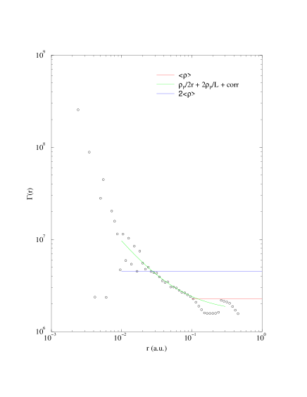
Figure 12: The conditional density for the egg-crate model universe (in the horizontal axis distances are in arbitrary units (a.u.)) $\langle\rho\rangle$ is the average density. This function shows a power law behavior up to $L=0.1$ and then it flattens towards a constant value. The dotted line shows the analytic prediction for such a model.

ii) The quantity $r_{0}$ in Eq.53 is a physically real characteristic length for the distribution, and it should be independent on the sample size. iii) According to Eq.53 one should find structures and voids of one order of magnitude larger than the correlation length $r_{0}$, i.e. up to $L\sim 50h^{-1}Mpc$, while this is not the case for real galaxy structures. Of course, the difference between $r_{0}$ and $L$ is such a system is a consequence of a very particular distribution (cubic lattice of uniform planes) that is different from the observed one.

In real galaxy and cluster catalogs we find that the conditional density does not show any tendency towards homogenization in any of the available samples, and that $r_{0}$ is indeed a linear function of the sample size.

3 Correlation analysis for galaxy distributions

In this section we discuss the correlation properties of the galaxy distributions in terms of volume limited catalogs [18] arising from about 100.000 redshift measurements that have been made to date. To this end, we study the behavior of the conditional (average) density, that is the main statistical tool useful to characterize the properties of highly inhomogeneous systems as well as regular ones. In particular, this statistical quantity is the appropriate one to identify self-similar properties, if they are present in the distribution.

A first important result is that the samples are statistically rather good and their properties are in agreement with each other. This gives a new perspective because, using the standard methods of analysis, the properties of different samples appear contradictory with each other and, often, this is considered to be a problem of the data (unfair samples) while, we show that this is due to the inappropriate methods of analysis. In addition, all the galaxy and cluster catalogs show well defined scale-invariant correlations up to their limits ($\sim 150h^{-1}Mpc$) and the fractal dimension is $D\approx 2$. We refer to Sec.6 for a complete summary of all the available redshift samples.

3.1 Detailed analysis of the available catalogs

A three dimensional catalog contains for each galaxy the two angular coordinates $\alpha,\delta$, the redshift $z$ and the apparent magnitude $m$. The analyses presented in this review are, in general, performed in galactic coordinates $(b,l)$, using, if needed, the limitation $|b|>10^{\circ}$. In such a way we can exclude the region corresponding to the galactic plane, where, because of dust absorption, it is problematic to measure redshifts.

We introduce some basic definitions. If $L$ is the absolute or intrinsic luminosity of a galaxy at distance $r$, this appears with an apparent flux

$$f=\frac{L}{4\pi r^{2}}\;.$$ (54)

For historical reasons the apparent magnitude $m$ of an object with incoming flux $f$ is

$$m=-2.5\log_{10}f+constant,$$ (55)

while the absolute magnitude $M$ is instead related to its intrinsic luminosity $L$ by

$$M=-2.5\log_{10}L+constant^{\prime}.$$ (56)

From Eq.54 it follows that the difference between the apparent and the absolute magnitudes of an object at distance $r$ is (at relatively small distances, neglecting relativistic effects)

$$m-M=5\log_{10}r+25$$ (57)

where $r$ is expressed in Megaparsec ($1Mpc=3\cdot 10^{24}\;cm$).

A catalog is usually obtained by measuring the redshifts of the all galaxies with apparent magnitude brighter than a certain apparent magnitude limit $m_{lim}$, in a certain region of the sky defined by a solid angle $\Omega$. An important selection effect exists, in that at every distance in the apparent magnitude limited survey, there is a definite limit in intrinsic luminosity which is the absolute magnitude of the fainter galaxy which can be seen at that distance. Hence at large distances, intrinsically faint objects are not observed whereas at smaller distances they are observed. In order to analyze the statistical properties of galaxy distribution, a catalog which does not suffer for this selection effect must be used. In general, it exists a very well known procedure to obtain a sample that is not biased by this luminosity selection effect: this is the so-called ”volume limited” (VL) sample. A VL sample contains every galaxy in the volume which is more luminous than a certain limit, so that in such a sample there is no incompleteness for an observational luminosity selection effect [18, 2]. Such a sample is defined by a certain maximum distance $R_{VL}$ and the absolute magnitude limit $M_{VL}$ given by

$$M_{VL}=m_{lim}-5\log_{10}R_{VL}-25-A(z)$$ (58)

where $A(z)$ takes into account various corrections (K-corrections, absorption, relativistic effects, etc.), and $m_{lim}$ is the survey apparent magnitude limit. (In Sec.2.4, we have defined the effective depth $R_{eff}$ for the analysis of a sample.) Different VL samples, extracted from one catalog, have different $R_{eff}$, and deeper is a VL sample, larger its $R_{eff}$. The (geometrical) limit of validity of the whole catalog is then the largest $R_{eff}$ that corresponds to the deepest VL sample with a robust statistics (we refer to Sec.5 for a discussion of the statistical fairness of samples).

The measured velocities of the galaxies have been expressed in the preferred frame of the Cosmic Microwave Background Radiation (CMBR), i.e. the heliocentric velocities of the galaxies have been corrected for the solar motion with respect to the CMBR, according with the formula

$$\vec{v}=\vec{v}_{m}+316cos\theta\;\;kms^{-1}$$ (59)

where $\vec{v}$ is the corrected velocity, $\vec{v}_{m}$ is the observed velocity and $\theta$ is the angle between the observed velocity and the direction of the CMBR dipole anisotropy ($\alpha=169.5^{\circ}$ and $\delta=-7.5^{\circ}$). From these corrected velocities, we have calculated the comoving distances $r(z)$, with for example $q_{0}=0.5$, by using the Mattig’s relation [9]

$$r(z)=6000\left(1-\frac{1}{\sqrt{(1+z)}}\right)h^{-1}Mpc\;.$$ (60)

In general, we have checked that the results of our analysis depend very weakly on the particular value of $q_{0}$ adopted, except very deep surveys, and we have also used the simple linear relation

$$r=cz/H_{0}\;.$$ (61)

In the nearby catalogs there is no any sensible change by using Eq.61 instead of Eq.60. Hereafter for the Hubble constant (unless it is not explicitly stressed), we use the value $H_{0}=100\cdot h\cdot kmsec^{-1}Mpc^{-1}$.

All the analyses presented here have been performed in redshift space and we have not adopted any correction to take into account the eventual effect of peculiar velocities (local distortion to the Hubble flow). However we point out that peculiar velocities have an amplitude up to $\sim 500\div 1000kmsec^{-1}$ and then their effect can be important only up to $5\div 10h^{-1}Mpc$, and not more.

We briefly mention the characteristics of the galaxy luminosity distribution that is useful in what follows analyses. The basic assumption we use to compute all the following relations is that:

$$\nu(L,\vec{r})=\phi(L)\rho(\vec{r})\;,$$ (62)

i.e. that the number of galaxies for unit luminosity and volume $\nu(L,\vec{r})$ can be expressed as the product of the space density $\rho(\vec{r})$ and the luminosity function $\phi(L)$ ($L$ is the intrinsic luminosity). This is a crude approximation in view of the multifractal properties of the distribution (correlation between position and luminosity), and a detailed discussion can be found in Sec.8. However, for the purpose of the present discussion, the approximation of Eq.62 is rather good and the explicit consideration of the multifractal properties have a minor effect on the properties we discuss [47].

To each VL sample (limited by the absolute magnitude $M_{VL}$) we can associate the luminosity factor

$$\Phi(M_{VL})=\int_{-\infty}^{M_{VL}}\phi(M)dM$$ (63)

that gives the fraction of galaxies for unit volume, present in the sample. Hereafter we adopt the following normalization for the luminosity function

$$\Phi(\infty)=\int_{-\infty}^{M_{min}}\phi(M)dM=1$$ (64)

where $M_{min}\approx-10\div-12$ is the fainter galaxy present in the available samples. The luminosity factor of Eq.63 is useful to normalize the space density in different VL samples which have different $M_{VL}$ (Eq.58). The luminosity function measured in real catalogs has the so-called Schecther like shape (sec.8) [48]

$$\phi(M)dM=A\cdot 10^{-0.4(\delta+1)M}e^{-10^{0.4(M^{*}-M)}}dM$$ (65)

where $\delta\approx-1.1$ and $M^{*}\approx-19.5$ [37] [44], and the constant $A$ is given by the normalization condition of Eq.64 (we refer to Sec.8 for a more detailed discussion of this subject).

The scheme of the analyses presented in the next section is the following. We extract from the catalog several VL samples and we study:

• The average conditional density $\Gamma(r)$ and the integrated conditional density $\Gamma^{*}(r)$. In such a way we determine the fractal dimension and detect, if present, the eventual crossover towards homogenization. Moreover, we present some tests to check the statistical stability of the results versus the possible incompleteness and systematic errors that could be present in the data.

• Determination $\xi(r)$; in this way we can definitely establish which kind of statistical information such a function gives.

• Determination of the dependence of the so-called ”correlation length” $r_{0}$, defined as $\xi(r_{0})\equiv 1$, on the sample depth $R_{eff}$. We study also its eventual dependence on luminosity (i.e the so-called luminosity segregation phenomenon).

• We refer to the Appendix for a detailed description of the VL samples of the various catalogs.

3.1.1 CfA1

The CfA1 catalog has been the first wide angle redshift survey ($\Omega=1.83\;sr$) available in the literature [17]. Coleman, Pietronero and Sanders in 1988 [21] have analyzed this catalog with the methods of modern statistical mechanics. They found in this sample galaxy distribution shows power law (fractal) correlations up to the sample limit of $20h^{-1}Mpc$ without any tendency towards homogenization. In particular the main results are:

i) The CfA1 catalog is statistically a fair sample up to $\>\sim 20h^{-1}Mpc$: a sample is statistically fair if it is possible to extract from it an information that is statistically meaningful. Whether it is homogeneous or not, it is a property that can be tested and it is independent on sample statistical fairness (Sec.5).

ii) $\Gamma(r)$ shows a well defined power law (fractal) behavior up to the sample limit, $R_{eff}\sim 20h^{-1}Mpc$, (Fig.13) without any tendency towards homogenization. For CfA1 $\>\gamma=3-D\sim 1.1\pm 0.2$ and the fractal dimension is $\>D=1.9\pm 0.2$ (when measured by the $\Gamma^{*}(r)$). The small discrepancy with the value reported by [2] (i.e. $D\sim 1.4\pm 0.1$) is due basically to the fact that we have used $\Gamma^{*}(r)$ rather than $\Gamma(r)$ to estimate the correlation exponent. Moreover, we have used a logarithm variable value of $\Delta r$ (the thickness of the shell in which the conditional density is computed): in more dilute samples, like those of CfA1, such a procedure gives a more stable result for the correlation exponent (Sec.2.4).

Figure 13: The conditional average density $\Gamma^{*}(r)$ for the sample VL40 and VL80 of CfA1. The reference line has a slope $-\gamma=-1.1$.

iii) The linear dependence of $\>r_{0}$ on the sample size $\>R_{eff}$ has been found (Fig.14)

Figure 14: The so-called ”correlation length” $r_{0}$ as a function of the sample size $R_{eff}$. The reference line has a slope $1$, in agreement with the behavior for a fractal distribution.

in the whole CfA1 catalog [21, 2] and it is naturally explained by the the fractal nature of the galaxies distribution in this sample. The extended CfA2 survey can proof (or not) this relationship over larger distances.

Davis et al.[49] have reached a different conclusion. In agreement with our results, they found that $r_{0}$ increases with the sample depth. However the slope of linear regression between $\log r_{0}$ and $\log R_{eff}$ they find is slightly smaller than 1. In fact, their data are more consistent with an exponent of about 0.7-0.8 instead of 0.5 as the authors claim. (This can be seen in their Table 1). This minor discrepancy with the exponent 1 is probably due to their way of treating the boundary conditions (i.e. weighting schemes), which, as we show later, introduces spurious homogenization, and thus a systematic decrease of the $r_{0}$ scaling. However the CfA2 catalog, as other deeper redshift samples, allows us to clarify also this controversial result.

3.1.2 CfA2

The extended CfA survey represents currently one of most complete catalog of visible matter distribution in the nearby Universe. In this survey it is possible to study the large scale structures distribution up to $\approx 150h^{-1}Mpc$. Since this survey is not yet published, we comment about the results of the analyses performed by various authors. Moreover we refer to Sec.4 for a discussion on the power spectrum results.

The old CfA survey (CfA1) is limited by an apparent magnitude of $\>m_{b(0)}\leq 14.5$ and contains about 1800 galaxies. The extension of the CfA redshift survey is up to $\>m_{b(0)}\leq 15.5$ and includes $\>\sim 11000$ galaxies ($6478$ galaxies CfA North and $\>4283$ galaxies CfA south). The main papers published about the CfA2 data analysis to which we refer are [36, 50, 37, 38].

The details on the subsamples used in the CfA2 data analysis are the following (from [38]). The VL subsamples correspond to depths $\>R_{s}=130h^{-1}Mpc$ (CfA2-130), 101 (CfA2-101), 78.1 (CfA2-78), and 60 (CfA2-60), respectively. The absolute magnitude limit for CfA130 is $\>M=-20.3$: this sample has the same absolute magnitude limit of the VL sample CfA1-80 of CfA1 (CfA1-80 means that $R_{VL}=80h^{-1}Mpc$).

In [38] the correlation function $\xi(r)$ (CF hereafter) has been estimated from direct pair count distribution, normalizing these counts to those for a random distribution of points within the survey volume [18]. In Figure 10 of [38] (Fig.15)

Figure 15: The correlation function $\xi(r)$ for two VL samples of CfA2: VL101 and VL130 (from Park et al.1994). The fitting curve are computed from the $\xi(r)$ function for a fractal distribution. The correlation exponent, in both cases, is $\gamma=1$, which corresponds to a fractal dimension $D=2$.

it is shown the CF for two VL subsamples, CfA101 and CfA130. The results of the CF-analysis are the following:

i) As shown in Fig.15, the exponent of the CF $\>\xi(r)$ is $\>\gamma\sim 1.0$ so that the fractal dimension is $\>D\sim 2=3-\gamma$ in the range between $\>2h^{-1}Mpc$ and $\approx 10h^{-1}Mpc$ in agreement with the results of the PS (Sec.4).

ii) The so-called correlation length $\>r_{0}$, defined as $\>\xi(r_{0})\equiv 1$, is $r_{0}\sim 7h^{-1}Mpc$ for CfA2-101, and $r_{0}\sim 10h^{-1}Mpc$ for CfA2-130. The amplitude of the CF for CfA2-130 is approximately $\>40\%$ higher than amplitude of the CF for CfA2-101, in agreement with the larger amplitude they find for the power spectrum for the same subsamples. The amplitudes of the CF in the two subsamples CfA2-130 and CfA2-101 are different and scale linearly with sample depth. This is the same result found at lower distances: the so-called correlation length $\>r_{0}$ is a linear function of the survey depth, if the system has fractal properties, and it scales up to $\>10h^{-1}Mpc$ for the deeper sample (CfA2-130). Note that not only the functional behavior, but also the values of $r_{0}$ is in agreement with the prediction for a fractal with $D=2$: $r_{0}\approx R_{eff}/3$. The value of the effective depth depends on the solid angle; this is $\Omega\approx 1.1$ and $R_{eff}\approx 30h^{-1}Mpc$ for CfA2-130, and $R_{eff}\approx 20h^{-1}Mpc$ for CfA2-101. Therefore the linear dependence of $r_{0}$ on the sample depth $R_{eff}$ is confirmed over the range of CfA1 and extended up the deeper depth of CfA2.

The authors [38] comment that the amplitude of clustering may depend on the luminosity of galaxies, because in the CfA130 subsample the absolute magnitude of the galaxies is in average higher than for the galaxies in CfA101. We discuss this point later, but now we can go further by comparing the sample of the new catalog CfA2-130 with the VL sample of the old catalog CfA1-80: these samples have the same absolute magnitude limit. Hence if these samples contain galaxies with the same distribution of absolute magnitude but they have different depth, we can then test the following hypothesis: if the amplitude of the CF depends on the brightness of galaxies one expects to find the same amplitude in both the subsamples (CfA2-130 and CfA1-80) otherwise, if the scaling of the amplitude of CF linearly depends on the sample depth, one expects to find a linear proportion between amplitudes and depths. It is easy to show that the second hypothesis is the case.

3.1.3 Perseus-Pisces

We have studied the behavior of $\>\Gamma(r)$ and $\>\Gamma^{*}(r)$ in several VL subsamples extracted from the Perseus-Pisces (hereafter PP) survey limited at the magnitude $m_{b}=15.5$ (see Appendix) [51]. The total number of galaxies contained in such a sample is $3301$ and the solid angle is $\Omega=0.9\;sr$. The effective depth (i.e. the radius of the maximum sphere fully contained in the sample) is $R_{eff}\approx 30h^{-1}Mpc$. The results are shown in Fig.16.

Figure 16: The average conditional density $\Gamma^{*}(r)$ plotted as a function of the length scale for various volume limited of Perseus-Pisces: VL60, VL80, VL100. The difference in amplitude is simply due to the different luminosity selection in the various VL samples, and can be renormalized by taking into account the different luminosity factor of these subsamples. A reference slope of $-\gamma=-0.9$ is indicated by the dashed line. The fractal dimension of these samples turns out to be $D=2.1$ up to $\sim 30\>h^{-1}Mpc$.

A well defined power law behavior is detected up to the sample limit ($R_{eff}\sim 30h^{-1}Mpc$) without any tendency towards homogenization. The codimension is, with very good accuracy, $\gamma=3-D\approx 0.9$ so that $\>D\approx 2.1$. Hence the PP redshift survey shows well defined fractal properties up to the effective depth $\>R_{eff}\approx 30h^{-1}Mpc$. It has consistent statistical properties and hence it is a statistically fair and not homogeneous sample [51].

We can clarify here an important technical point in the computation of the conditional density. Guzzo et al.[89], by measuring $\Gamma(r)$ in this catalog, have found a change of slope at $\sim 2h^{-1}Mpc$ : in particular they found that, at these small scales, $D=1.2$ rather than with $D\approx 2$. In order to understand why this change of slope occurs, we recall that, in the estimate of the conditional density one computes the density in a shell of thickness $\Delta r$ at distance $r$ from every occupied point, and then one performs the average. When one computes this quantity in real cases, one should define the appropriate value for $\Delta r$. At small distances we are below the average minimum separation between nearest galaxies in the sample that is of the order of some Megaparsec, depending on the sample considered. For example for the various volume limited samples of Peruses-Pisces this number is in the range $1\div 4h^{-1}Mpc$. At very small distances one underestimates the number of galaxies in the shell of thickness $\Delta r$ for a finite size effect that causes a steeper behavior for $\Gamma(r)$. This finite size effect is the real reason for the change of slope (Sec.2.4).

As we have already discussed in Sec.2.4 (see also [2]), we have limited our analysis to an effective depth $R_{eff}$ that is of the order of the radius of the maximum sphere fully contained in the sample volume. In such a way we eliminate from the statistics the points for which a sphere of radius r is not fully included within the sample boundaries. Doing so we do not make any assumption on the treatment of the boundaries conditions. Of course in doing this, we have a smaller number of points and we stop our analysis at a smaller depth than that of other authors [52], with the advantage, however, of not introducing any a priori hypothesis.

The different normalization in the various VL samples is due to the different absolute magnitude limit ($M_{VL}$) that define each VL subsample. To normalize the density $\Gamma(r)$, we divide it for a luminosity factor given by Eq.63 (we refer to Sec.6.4. for a detailed discussion of such a normalization).

We have studied the $\>\xi(r)$ function in the VL subsamples with different depth. We find that for $\>r\mathrel{\hbox to0.0pt{\lower 3.0pt\hbox{$\mathchar 536\relax$}\hss}\raise 2.0pt\hbox{$\mathchar 316\relax$}}r_{0}$ $\>\gamma\approx 1$. The amplitude of $\>\xi(r)$ is sample depth dependent: in Fig.17

Figure 17: The ”Characteristic length scale” $r_{0}$ ($\xi(r_{0})\equiv 1$) plotted as a function of the effective radius $R_{eff}$ for the samples of PP. If the catalog is homogeneous we should find a constant value for $r_{0}$. The fitting line has a slope of $(D/6)^{\frac{1}{3-D}}$ as predicted for the fractal case.

the behavior of $\>r_{0}$ is plotted as a function of the sample depth $\>R_{eff}$ for the VL samples of PP. The experimental data are very well fitted by the prediction for a fractal distribution. This analysis is in agreement with the one of [2] and with the analysis done by the CF $\>\Gamma(r)$ discussed previously. The so-called ”correlation length” $\>r_{0}$ has therefore no physical meaning but it only represents a fraction of the sample size (we refer to Sec.3.3 for a test on luminosity segregation).

3.1.4 SSRS1

This sample consists of 1773 galaxies covering an area of $\Omega=1.75\;sr$ of the South galactic cap in the region south of declination $-17^{\circ}.5$ and below galactic latitude $-30^{\circ}$ [39, 53]. The sample is complete down to a limiting galactic diameter given by $\log[D(0)]=0.1$, where $D(0)$ is in arcminutes.

The galaxy distribution exhibits prominent structures and large scale voids, delimited only by the extension of the survey: ”….we can now recognize that the distribution of galaxies is very inhomogeneous ….” [39]. A clear dependence of $r_{0}$ on the sample depth has been found also in this survey [54]. However the authors [54] attribute the scaling with depth of $r_{0}$ to the ”luminosity segregation” phenomenon.

In order to investigate this point we have extracted from the catalog various samples which are complete in absolute diameter (analogous a VL sample). We have considered the subsamples which have a depth of $40,60,80,100$ and $120h^{-1}Mpc$ (see Appendix). The radius of the maximum sphere fully contained in the deepest subsample, which is the limit of our statistical analysis, is $R_{eff}\sim 35h^{-1}Mpc$. We have computed the conditional average density and the conditional density for the various subsamples and we show the results in Fig.18.

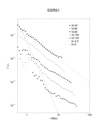
Figure 18: The average conditional density $\Gamma^{*}(r)$ plotted as a function of the length scale for various volume limited of SSRS1. A reference slope of $-\gamma=-1$ is indicated by the dashed line, that corresponds to a fractal dimension of $D\approx 2$ up to $35\>h^{-1}Mpc$. The dashed line has a slope $-3$ (D=0).

We find that galaxy distribution in this sample is characterized by having long range correlations up to $\sim 35h^{-1}Mpc$, with fractal dimension $D=2.0\pm 0.1$. We find no evidence for a crossover towards homogenization in this catalog. The deepest sample VL120 has a very poor statistics, and this is the reason why $\Gamma^{*}(r)$ is more noisy and has a $1/r^{3}$ decay at small distances (Sec.2.1.2 and Sec.5 for a detailed discussion of such an effect). This small scale behavior is due to the fact that, in this sample, in average one does not find any other galaxy for $r\mathrel{\hbox to0.0pt{\lower 3.0pt\hbox{$\mathchar 536\relax$}\hss}\raise 2.0pt\hbox{$\mathchar 316\relax$}}7h^{-1}Mpc$. The conditional average density for the sample VL120 is smoother and shows a complete agreement with the all the other samples.

We have then computed the so-called ”correlation length” by performing the standard correlation analysis by the $\xi(r)$ function. As shown in Fig.19, we have studied $\>\xi(r)$ in the VL samples with different depth. We find that the amplitude of $\>\xi(r)$ is sample depth dependent.

Figure 19: The ”Characteristic length scale” $r_{0}$ ($\xi(r_{0})\equiv 1$) plotted as a function of the effective radius $R_{s}$ for the samples of SSRS1. The fitting line has a slope of $(D/6)^{\frac{1}{3-D}}$ as predicted for the fractal case.

Even in this case the experimental data are very well fitted by the prediction for a fractal distribution (Sec.2.3). Contrary to the results of Maurogordato, Schaeffer and da Costa [54], from the previous tests, we find no evidence for a luminosity dependence of $r_{0}$. Rather we find, in agreement with the correlation analysis performed by the $\Gamma(r)$ function, that $r_{0}$ is a fraction of the sample size, as expected in the fractal case.

3.1.5 SSRS2

The SSRS2 catalog is a magnitude limited survey that includes $\sim 3600$ galaxies and covers $\Omega=1.13\;sr$, complete up to limiting magnitude $m_{B(0)}=15.5$ [37, 55] (this catalog is not yet published). The characteristics of the VL samples are reported in the Appendix. In the first paper about this survey [37], the authors concluded that ”by examining the normalizing density fluctuations in the SSRS2 and CfA2 surveys we suggest that the combined sample is not large enough to be fair: there are large fluctuations (i.e. the South Wall) in shells at $100h^{-1}Mpc$”. It is clear that, even in this case, the sample is declared to be ”not fair” because it does not show a well defined average density, but on the contrary it is dominated by fluctuations as large as the sample itself.

Benoist et al.[55] have measured the ”correlation length” $r_{0}$ in several VL samples of different depth. We show in Tab.1

Sample	$r_{0}(h^{-1}Mpc)$	$R_{eff}(h^{-1}Mpc)$
D48	$3.5\pm 0.2$	12
D60	$4.8\pm 0.5$	15
D74	$5.5\pm 0.4$	18
D91	$5.8\pm 0.6$	22
D112	$5.5\pm 0.6$	27
D138	$8.0\pm 0.4$	36
D168	$15.8\pm 2.9$	40

Table 1: Values of $r_{0}$ and $R_{eff}$ (which has been estimated by knowing the geometry of the sample) for the various VL samples of the SSRS2 survey (from Benoist et al.1996). There is a clear dependence of $r_{0}$ on the sample depth.

the values of $r_{0}$ and $R_{eff}$ for the various VL samples of the SSRS2 survey. A clear dependence of $r_{0}$ on sample size is shown. We stress that the authors [55] fit the $\xi(r)$ with a power law behavior in the wrong region of length scales, i.e. for $r\approx r_{0}$, and hence they find a higher value for the correlation exponent $\gamma\approx 1.5\div 1.8$ (Sec.2.3). By fitting the $\xi(r)$ function with the expected shape for a fractal distribution we find that there is a very good agreement with the published data: we show in Fig.20

Figure 20: The $\xi(r)$ function for SSRS2 in the VL samples D30, D138 and D168 (from Benoist et al.1996). The fitting curve has been compute from the expression of $\xi(r)$ for a fractal distribution. In all the cases the slope is $\gamma=1$, i.e. the fractal dimension is $D=2$.

the $\xi(r)$ for several VL samples of SSRS2 together with a fitting curve that is $\xi(r)=[(3-\gamma)/3](r/R_{eff})^{-\gamma}-1$, and the value of the exponent is $-\gamma=-1$ in all the cases. We can then conclude that the fractal dimension in this case is again $D\approx 2$.

Let us come to the discussion of the scaling of $r_{0}$ in the various VL samples. First of all we notice that $r_{0}\approx 16h^{-1}Mpc$ is the highest value for the correlation length ever found in a redshift survey, after the results of LEDA [24]. The authors [55] have done several test in order to check if the dependence of $r_{0}$ on sample size is due to a luminosity effect or to a depth effect. In the first case it should be due to the so-called luminosity segregation phenomenon, while in the second case it should be attributed to the intrinsic fractal nature of galaxy distribution in this sample.

First of all we stress that in all the galaxy surveys, such as CfA1 and SSRS1 for example, there are galaxies with $M\leq-19.5$ because these are the most luminous ones. However, in no one of these catalogs a value of $r_{0}\approx 16h^{-1}Mpc$ has been ever measured. If luminosity segregation is the real physical effect that produces the scaling of $r_{0}$, then such a value of $r_{0}$ should be present in all the other surveys, as it refers to the most luminous galaxies.

On the contrary, the authors [55] conclude that the variation of the $\xi(r)$ amplitude, observed in this catalog has two contributions: sampling fluctuation for the faint galaxies, and luminosity segregation for the brighter ones. However we can make the following comments on these results: i) The authors do not present any quantitative argument that explains the shift of $r_{0}$ with sample size (Fig.1 of [55]), but they just make several test on the deeper samples that seem to show a difference in the amplitude of $\xi(r)$ for brighter and fainter galaxies. ii) The test only on luminosity segregation that gives a result that seems to be in agreement with such an effect (but without any quantitative discussion), is performed only in the sample D91 that contains 67 galaxies in the magnitude bin $-21.5/-20.5$ (Fig.2 of [55]): they stress in fact that ”only in the large VL (D91) we found a significant effect”. They do not show the results for the deeper samples, nor they find a consistent argument that can explain why the amplitude of the correlation function reaches the value $r_{0}\sim 16h^{-1}Mpc$. iii) In Fig.3 of [55] it is reported the behavior of $\xi(r)$ for galaxies in the same interval of absolute magnitude but in samples with different depth. About these results, we can comment that they have computed the $\xi(r)$ function by using the standard method of treatment of boundary conditions in samples with a small difference in the effective depth $R_{eff}$ (see Tab.1 and their Fig.3). Hence it is very difficult to make definitive conclusions from their analyses. iv) Moreover the authors [55] do not present the computation of $\Gamma(r)$ that is the clarifying test, in order to check the fractal versus homogeneous properties in this sample.

We came back on the problem of ”luminosity segregation” later by performing several specific tests. We stress again that this effect has been invoked by several authors [38, 55] to explain the shift of the amplitude of $\xi(r)$ or of the power spectrum in samples of different depth (and different average absolute magnitude), but in any case it has never been presented any quantitative argument that can explain the behavior of the amplitude of $\xi(r)$ with absolute luminosity.

Instead, in the case of SSRS2, we cannot present here a detailed analysis because the survey is not yet published, but we can argue from the available results of the data analysis that galaxy distribution in SSRS2 is fractal with dimension $D\approx 2$ up to the limiting depth of $R_{eff}\sim 50h^{-1}Mpc$. A test that may proof such a behavior is the measure of the conditional density that should have a power law behavior with exponent $-\gamma\approx-1$, i.e. $D\approx 2$, up to $\sim 50h^{-1}Mpc$.

3.1.6 Stromlo-APM

The Stromlo-APM Redshift Survey (SARS) consists of 1797 with $b_{J}\leq 17.15$ selected randomly at a rate of 1 in 20 from APM scans [56, 57]. The survey covers a solid angle of $\Omega=1.3sr$ in the south galactic hemisphere, delimited by $21^{h}\mathrel{\hbox to0.0pt{\lower 3.0pt\hbox{$\mathchar 536\relax$}\hss}\raise 2.0pt\hbox{$\mathchar 316\relax$}}\alpha\mathrel{\hbox to0.0pt{\lower 3.0pt\hbox{$\mathchar 536\relax$}\hss}\raise 2.0pt\hbox{$\mathchar 316\relax$}}5^{h}$ and $-72.5^{\circ}\mathrel{\hbox to0.0pt{\lower 3.0pt\hbox{$\mathchar 536\relax$}\hss}\raise 2.0pt\hbox{$\mathchar 316\relax$}}\delta\mathrel{\hbox to0.0pt{\lower 3.0pt\hbox{$\mathchar 536\relax$}\hss}\raise 2.0pt\hbox{$\mathchar 316\relax$}}-17.5^{\circ}$ (see Appendix). An important selection effects exists: galaxies with apparent magnitude brighter than $b_{j}=14.5$ are not included in the sample because of photographic saturation (see Fig.21).

Figure 21: Absolute magnitude versus distance diagram for the SARS catalog. There are shown the two limiting function with apparent magnitude $m^{1}_{lim}=14.5$ and $m^{2}_{lim}=17.15$. The survey is complete up to $\sim 17-th$ magnitude and does not contain galaxies brighter than $\sim 14.5$.

In order to construct VL samples we have adopted two different procedures. The first is the standard one, i.e. we have introduced an upper cutoff in the distance and computed the corresponding cutoff in absolute magnitude (see Appendix). The second consists by putting two limits in distances and compute the corresponding two limits in absolute magnitude. In such a way we can avoid the selection effects due to the fact that in this survey are not included galaxies brighter than $14.5$ (this is the same procedure used in the case of LCRS that is limited by a lower and an upper limit in apparent magnitude as SARS).

We have then computed the conditional average density for the VL samples with only one cut in absolute magnitude, and we show in Fig.22 the results.

Figure 22: The conditional average density computed for some VL sample of the SARS redshift survey. The reference line has a slope $-\gamma=-0.8$. The fractal dimension is $D=2.2\pm 0.2$, depending on the VL sample used.

The fractal dimension is $D=2.2\pm 0.2$ up to $\sim 35h^{-1}Mpc$. From the previous figure it follows that the conditional density for the deeper VL sample (VL20, where 20 refers to the absolute magnitude limit of the VL sample) has a tendency towards a flattening at scales larger than $\mathrel{\hbox to0.0pt{\lower 3.0pt\hbox{$\mathchar 536\relax$}\hss}\raise 2.0pt\hbox{$\mathchar 318\relax$}}30h^{-1}Mpc$. Such a flattening in our view is completely spurious and due to the sparseness of this particular sample. We refer to Sec.5 for a detailed discussion of this effect.

In order to check that the luminosity incompleteness of the sample for apparent magnitude brighter than $14.5$ affects substantially the trends found in Fig.22, we have computed the conditional average density for the VL samples, with two cuts in distance and two in absolute magnitude. These samples are defined by a lower and an upper cut in distance (for example VL100-200 means that we have cut the VL between the region from $100$ to $200h^{-1}Mpc$ - see Appendix).

Figure 23: The conditional average density computed for some VL sample of the SARS redshift survey, with two cuts in distance and absolute magnitude. Such a procedure avoids the luminosity incompleteness of galaxies with apparent magnitude brighter than $14.5$. The reference line has a slope $-\gamma=-0.8$. The fractal dimension is $D=2.2\pm 0.2$.

Even in this case (Fig.23) the fractal dimension turns out to be $D=2.2\pm 0.2$ up to $R_{eff}\sim 40h^{-1}Mpc$: some samples show a tendency towards a flattening. We can show by precise tests that this flattening is spurious and it is due to the sparseness and weak statistics of these samples (Sec.5).

3.1.7 LEDA

We have studied in a series of papers [24, 58, 59, 60, 61, 62] the statistical properties of there LEDA database, and here we review our main results. This database now contains more than 200,000 galaxies with the most important astrophysical parameters: name of galaxies, morphological description, diameters, axis ratios, magnitudes in different colors, radial velocities, 21-cm line widths, central velocity dispersions, etc. In the last 12 years since the inception of LEDA, more than 75,000 redshifts have been collected, for more than 40,000 galaxies.

The magnitudes of the galaxies registered in the LEDA database come from many different references. It is the aim of a database to collect all new measurements of galactic observational parameters. In the paper [63] the formulae to reduce twenty different magnitudes systems to the photoelectric $b_{t}$ system of the Third Reference Catalogue (RC3) are given. This reduction is done in such a way that the resulting magnitudes are completely free of bias or perturbing effects. Each magnitude is then given with its own error. This error is of course in the range 0.1 to 1 magnitude depending on the observations and on the comparison between different published values for the same galaxy. The majority of the galaxies have a mean error less than 0.5 magnitude. The complete list of the references of the magnitudes we used for the purpose of this paper can be found in [64] (we refer to this paper also for more information of the data contained in LEDA).

The main selection effect that must be studied with great care is the incompleteness of the redshift data in the LEDA database, for different directions of observation, i.e. a different angular incompleteness. In Fig.24, we show the percentage of galaxies

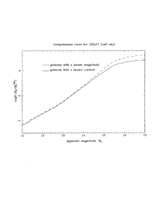
Figure 24: Fraction between the number of galaxies reported in LEDA and the number of galaxies with measured redshift. Up to $B\sim 14.5$ all the known galaxies are measured. After this limit the LEDA database begins to be incomplete.

known in angular catalogs compared to the number of galaxies having a measured redshift. Up to the limiting magnitude $m_{B}=14.5$, LEDA has a rate of redshift measurements of $90\%$, if we extend the study by including fainter galaxies up to a limit of $m_{B}=16$, this rate falls to $50\%$, and with $m_{B}$ limit $=17$, LEDA has only redshifts the $10\%$ of galaxies.

To investigate the incompleteness of the LEDA database we have built three magnitude limited (ML) samples: the first is limited at $m=14.5$ and it is called LEDA14.5, the second is limited at $m=16$ (LEDA16), and the third is limited at $m=17$ (LEDA17). The first ML subsample LEDA14.5 is almost complete, i.e. there are redshifts for the $\sim 90\%$ of the total number of galaxies present in the correspondent angular catalog. The problem that we discuss is whether the incompleteness in the deeper magnitude limited catalogs destroys the statistical relevance of the samples, or whether it is possible to recover the correct statistical properties and to control the effects of such incompleteness. In particular we perform several quantitative tests in order to clarify this crucial point.

In order to avoid the zones of avoidance due to the Milky Way, we cut the all-sky samples in two half-sky catalogs. In this way we have, for example, LEDA14.5N that refers to the northern galactic hemisphere, and LEDA14.5S that refers to the southern one. The samples denominated North and South are respectively selected with the galactic latitude: $b>+10^{\circ}$ and $b<-10^{\circ}$, as usually done in literature.

We have then 6 ML samples: LEDA14.5N and LEDA14.5S, LEDA16N and LEDA16S, LEDA17N and LEDA17S. We analyze separately each of these samples. Moreover to perform the space distribution analysis, we extract various VL samples and we report in the Appendix their characteristics. In such a way we have various independent VL samples.

In order to control the effect of the data incompleteness, we have firstly studied the correlation properties of the two VL samples extracted from LEDA14.5. These samples are nearly complete, and the incompleteness is no more than $\sim 10\%$. To compare our results with other known we have computed the correlation function in the same region of the CfA1 redshift survey. In this case we have a complete sample because LEDA contains the CfA1 redshift catalog. We find that the number of points in the various VL sample of LEDA14.5-CfA1 are nearly the same of that of CfA1. The conditional density scales as a power law with $\gamma=3-D=0.9\pm 0.2$ ($D=2.1\pm 0.2$) up to the sample limit that is $\sim 20h^{-1}Mpc$. The results of our analysis are therefore in perfect agreement with those of CfA1 (Sec.3.1.1).

The next step is to increase the solid of angle of the LEDA14.5N up to include all the northern hemisphere. We find that the CF function does not change neither its slope nor its amplitude, so that it remains a power law with the same fractal dimension. The scaling region extends up to $\sim 30h^{-1}Mpc$. Therefore in this way we can control the effect of incompleteness and conclude that this result confirms that the small incompleteness of this sample does not affect the correlation properties of galaxy distribution. Moreover, we have done the same analysis for the VL samples of LEDA14.5S finding a result in substantial agreement with that of LEDA14.5N. This implies that the statistical properties of the LEDA14.5 are robust with respect to the small incompleteness in the galaxy redshifts which characterize this sample. The fractal dimension in the VL sample of LEDA14.5 turns out to be $D=2.1\pm 0.2.$

An important point of the LEDA database analysis is that from the law of codimension additivity (Sec.2.2.4), it follows that if we cut points randomly from a fractal distribution, its fractal dimension does not change. The cutting procedure can be applied up to eliminate more than $\sim 95\%$ of the structure points without changing the genuine properties of the distribution (Sec.5). From the previous discussion, it follows that if the incompleteness effects are randomly distributed in space, they do not affect the correlation properties of the sample, unless the percentage of the points present in the sample is too small. On the contrary, if there are some systematic effects, as a poor sampling in certain large scale regions, the correlation properties can be seriously affected. This means that if in the incomplete samples we find the same correlation properties of the complete ones, we can be confident that we are measuring the real properties of galaxy distribution. Otherwise, if we detect an eventual cut-off towards homogenization we have to do a very careful analysis, to understand whether such a cut-off is spurious, i.e. do to systematic incompleteness effects, or whether it is an intrinsic property of the sample.

The amplitude of $\Gamma(r)$ is related to the lower cut-off of the distribution, i.e. to the prefactor of the average density. To normalize the conditional density in different VL samples (defined by the absolute magnitude limit $M_{VL}$) we divide it by the luminosity factor (we Sec.6.5 for a detailed discussion of such a normalization). In Fig.25

Figure 25: The conditional average density $\Gamma^{*}(r)$ for various VL samples of the LEDA14.5 sample. $N$ for the VL sample of the Northern hemisphere and $S$ for the Southern one. The reference line has a slope $-\gamma=-0.9$ ($D=2.1$).

there are plotted also the different $\Gamma(r)$ for the various VL samples of LEDA14.5: we find that there is a nice matching of the amplitudes and slopes. This implies that we are computing the correct galaxy conditional density in each subsample, and that such a quantity does not depend (or it depends very weakly) on the absolute magnitude of galaxies. Moreover we are confident to be not biased by any selection or incompleteness effect. We have done this kind of analysis for the whole north galactic hemisphere (LEDA14.5N) and for the southern one (LEDA14.5S): in both cases we obtain the same kind of behavior for $\Gamma(r)$.

The following step is to analyze the VL samples of LEDA16 (north and south), and we have studied the behavior of the correlation function $\Gamma(r)$ in the various VL samples of LEDA16N and LEDA16S. We find in both cases that the distribution has long-range correlation with the same fractal dimension $D=2.1\pm 0.2$, up to $\sim 80-90h^{-1}Mpc$ (Fig.26).

We stress that in some VL samples of LEDA16 (and also LEDA17) $\Gamma(r)$ is affected by incompleteness and it slightly deviates from a power law behavior. However we find that a power law behavior is quite stable in all the VL samples and we conclude that is some cases the incompleteness of the database may affect weakly the behavior of the conditional density. Such a conclusion is supported also by the power spectrum analysis (Sec.4).

To compare the amplitude of $\Gamma(r)$ in this samples we consider the normalized CF (i.e divided by the luminosity factor). We find that the amplitude of the normalized CF is about the $40\%$ of that found for LEDA14.5. This is because, in this case, the sampling rate is not $9/10$ as it is for LEDA14.5 but it is about $3/5$ as we have discussed previously. Hence a part this factor, we have that the CF has the same features of the one of LEDA14.5. Even in this case, we conclude that the incompleteness present in this sample are randomly distributed in the sky, and the correlation properties are only weakly affected by such effects.

Figure 26: The conditional average density $\Gamma^{*}(r)$ for various VL samples of the LEDA16 sample. $N$ for the VL sample of the Northern hemisphere and $S$ for the Southern one. The reference line has a slope $-\gamma=-0.9$.

Finally we consider the VL samples of LEDA17. For the deepest VL sample, we find that $\Gamma(r)$ has a power law behavior with $D=2.1\pm 0.2$ up to $\sim 150h^{-1}Mpc$ (Fig.27).

Figure 27: The conditional average density $\Gamma^{*}(r)$ for various VL samples of the LEDA17 sample. $N$ for the VL sample of the Northern hemisphere and $S$ for the Southern one. The reference line has a slope $-\gamma=-0.9$.

The correlation properties are substantially the same of the two previous cases. Therefore we conclude that this analysis show that the power law correlation cannot be an artifact due to the incompleteness of the sample.

We have performed another test in order to check the effects of the incompleteness. We have cut a VL sample in two region, for example, one up to $140h^{-1}Mpc$ and the other extending from $140$ to $280h^{-1}Mpc$. We then compute $\Gamma(r)$ in these two subsamples, and we find that the same power law behavior extending on all scales, up to the effective depth of the samples (Fig.28).

Figure 28: The conditional average density $\Gamma^{*}(r)$ for the VL sample VL280 (North) of LEDA16. The filled circles refer to the $\Gamma^{*}(r)$ of the total sample, the squares for the first half (0-140 $h^{-1}Mpc$) and the diamonds for the second half (140-280 $h^{-1}Mpc$).

This test shows that the correlation properties of the nearby sample are the same of the deepest one, and that the signal is stable. This behavior is exactly what one observes in a fractal distribution which shows the same properties in the environment of any occupied point. This is clearly different in the case of a radial incompleteness where the nearby points and the far away ones have different environments. We can conclude again that the incompleteness of the sample does not change the genuine behavior of the conditional average density.

We have performed also another test: we have cut one sample of LEDA14.5N and of LEDA14.5S at the limiting magnitude $M=-19$. Then we have measured $\Gamma(r)$: we find the same power law behavior in these two cases, and also the amplitudes match quite well. Then we have repeated the same procedure with LEDA16 and LEDA17, multiplying the amplitude of $\Gamma(r)$ for $0.5/0.9$ in the first case and $0.1/0.9$ in the second one. In such a way we have obtained 6 samples, all with the same magnitude limit $M=-19$: we find that all the amplitudes match quite well, confirming again the validity of the catalog.

In order to measure $\xi(r)$, we have adopted the same procedure used for the computation of $\Gamma(r)$. In fact we have firstly used the VL samples of LEDA14.5-CfA1, to compare the result with those of CP92. Then we have extended the analysis to the whole northern and southern hemispheres. Applying the same steps to LEDA16 and LEDA17, we find that in the deeper VL sample $r_{0}$ reached the value of $45\pm 5h^{-1}Mpc$ for a value of $R_{eff}\approx 150h^{-1}Mpc$ scaling as a linear function of the sample size Fig.29.

Figure 29: Behavior of the so-called ”correlation length” as a function of the sample size. The reference line has a linear behavior is in agreement with the fractal prediction. It is remarkable to note that in the deepest sample we find $r_{0}\approx 45\pm 5h^{-1}Mpc$.

This shows again that the usual $\xi(r)$ is completely misleading if applied to system characterized by long-range correlations. The so-called ”correlation length” $r_{0}$ is just an artifact due to an inconsistent mathematical analysis, and it is only a fraction of the sample size, so that it has no physical meaning.

3.1.8 Las Campanas

Las Campanas redshift survey (LCRS) is one of the deeper redshift survey available to date. This catalog covers a solid angle $\Omega=0.12\;sr$, and it is made of six $1.5^{\circ}\cdot 80^{\circ}$ slices, 3 in the north galactic hemisphere and 3 in the south. This survey contains more than $25000$ redshifts. However, there are several selection effects that must be considered with great detail. In fact, in any slice are mixed measurements performed with different instruments, which have different luminosity selections. Each slice is made of a number of different fields $1.5^{\circ}\cdot 1.5^{\circ}$. To each field it is associated a fraction $f$ that gives the ratio between the number of galaxies with measured redshift to the total number of galaxies in the field. In particular the most of the galaxy measurements are performed with apparent magnitude limit in the range $15\leq R\leq 17.7$, while for some fields it has been used the selection $15.0\leq R\leq 17.3$. Hence in each slice the fraction of galaxies measured is a function of the angular coordinates and apparent magnitude. We refer to [41] for a detailed discussion of the survey construction. In Fig.30 we show the absolute magnitude versus distance diagram for the six slices. It appears the double cut in apparent magnitude.

Figure 30: The absolute magnitude versus distance diagram for the six slices of LCRS. It is evident the double cut in apparent magnitude.

We have computed the conditional average density in each of the six slice of LCRS. In order to avoid the various selection effects, and to built an uniform sample, we have firstly analyzed the slice at $\delta=-12^{\circ}$ in the North galactic cap, that has been obtained with a more uniform selection (i.e. it has been done with the 112-fiber spectrograph). In such a slice the limits on the magnitude are $15\leq R\leq 17.7$. Then, in order to obtain the same galaxy sampling fraction among the various fields that constitute this slice, we have randomly eliminated galaxies from the different fields. In such a way we have obtained a uniform sample with sampling fraction $f\sim 0.5$.

We have then obtained some VL samples which are listed in the Appendix. For the construction of these samples we have an additional problem because galaxies are selected in a certain range of apparent magnitudes as in the case of APM. Hence a VL sample must be delimited by two cuts in distance and two in absolute magnitude. The behavior of the conditional average density is shown in Fig.31.

Figure 31: The conditional average density computed in several VL samples of the slice centered at $-12^{\circ}$. The reference line has a slope $-\gamma=-0.8$.

A clear power law behavior is obtained in the range of scales $0.5\div 15h^{-1}Mpc$. The radius of the maximum sphere fully contained in the sample volume is in this case $R_{eff}\sim 10h^{-1}Mpc$. The fractal dimension turns out to be $D=2.2\pm 0.2$. As the radius of the maximum sphere fully included in the sample volume is $R_{eff}\approx 10h^{-1}Mpc$, the corresponding value for the ”correlation length” is $r_{0}\approx 4h^{-1}Mpc$. We have performed the same analysis for the other five slices finding similar results, even if the signal is more noisy due to the different sampling fraction used in the construction of the various slices.

On the basis of the discussion presented in Sec.2.4., it is clear that the determination of the correlation function ($\Gamma(r)$ or $\xi(r)$) at scale $\sim 50\div 100h^{-1}Mpc$ or more is completely affected by the use of weighting schemes in treatment of boundary conditions, and does not contain any information about galaxy distribution in this sample [65].

3.1.9 ESP

The ESP survey consists of a strip $22^{\circ}\cdot 1.5^{\circ}$ plus a near-by area $\>5^{\circ}\cdot 1.5^{\circ}$ (five degrees west of the strip) in the South Galactic Pole region [44, 45]. The limiting magnitude of the survey is $\>b_{J}\leq 19.4$ and the total number of objects is $\>3601$. The survey area has been filled with a regular grid of circular fields with a diameter of $\>32$ arcminutes: this size corresponds to the field of view of the multifiber spectrograph at the ESO $\>3.6m$ telescope. The volume of the survey is very unusual: it does not cover a compact solid angle in the sky but, since it is made by a regular grid of circular fields, it has many ”holes” between a field and the following one. The total solid angle is $\Omega\approx 0.006sr$.

We have computed the conditional average density in various VL samples of ESP, limited at the strip $22^{\circ}\cdot 1.5^{\circ}$ (see Appendix). The radius of the maximum sphere fully enclosed in the deepest VL sample is $R_{eff}\approx 10h^{-1}Mpc$, so that it is possible to compute $\Gamma(r)$ only up to such distance. There is an additional problem in the case of ESP which requires a detailed investigation. In fact, as we have already stressed, the ESP survey is made of various crucial fields, and there are ”holes” between a field and its neighborhood. Unfortunately there is no way to correct for such a selection effect. In any case from Fig.32 it follows that

Figure 32: The conditional average density for various VL samples of ESP. A clear power law behavior is found up to $\sim 10h^{-1}Mpc$ with fractal dimension $D=1.8\pm 0.2$. The reference line has a slope $-\gamma=-1.2$.

that a clear power law behavior is found up to $\sim 10h^{-1}Mpc$ with $D=1.8\pm 0.2$. The presence of the holes may lead to a lower value of the fractal dimension in this survey.

3.1.10 IRAS $2Jy$ and IRAS $1.2Jy$ Redshift Surveys

The IRAS galaxies have been considered to be the unbiased tracers of matter distribution [66, 67] because the most infrared active galaxies are the spirals ones which are believed to be a better representation of the real matter distribution. The galaxy distribution of IRAS galaxies [68, 42] is dominated by the well-known superclusters: the Hydra-Centaurus-Pavo-Indus Supercluster forming together the so-called Great Attractor, and the Perseus-Pisces Supercluster. There are large voids in front of Perseus-Pisces Supercluster and off the supergalactic plane. It is remarkable that IRAS galaxies do not fill the voids, and, on the contrary, they trace the same structures of the optical ones. In particular it has been shown [68] very clearly that the large-scale distribution of IRAS and CfA, or SSRS, galaxies are very similar, and belong to the same structures.

The similar space distribution does not correspond to the same correlation properties of IRAS and optical samples. Optical galaxies, in fact, show long range power-law correlations up to a certain distance (see previous sections). The problem is therefore to understand why IRAS galaxies, that are located in the same structures of the optical ones, do not show the same correlation properties and, on the contrary, seem to have a very well defined constant density [68, 69] with a value of the so-called ”correlation length” of $r_{0}=4.5h^{-1}Mpc$. In particular, it has been shown that $r_{0}$ does not scale with sample depth [69]. This result is quite in contradiction with the linear dependence of $r_{0}$ on sample depth previously found.

The IRAS 2Jy survey (hereafter I-2) is a complete sample of galaxies uniformly selected over most of the sky. We refer the reader to [66, 68] for a detailed discussion of the sample selection. The sky coverage of the survey is $11.01sr$. The selection criteria have been chosen in relation to the infrared flux, and in particular there have been selected the galaxies with apparent flux at $60\mu m$ ($f_{60}$) greater than $1.936Jy$. This sample contains $2652$ galaxies. The IRAS 1.2 Jy survey (hereafter I-12) is a similar catalog, but it collects all the galaxies with $f_{60}>1.2Jy$, and the number of galaxies is doubled, and contains 5313 redshifts [42]. For the well-calibrated fluxes and the lack of Galactic extinction in the IRAS wavelengths, these surveys are believed to be well suited for studies of large scale distribution of galaxies.

We have studied [23] the space correlation properties of the various VL samples (see Appendix) and in particular we have computed the conditional average density. In Fig.33 there are shown the case of I-2

Figure 33: The conditional average density $\Gamma^{*}(r)$ computed in various VL samples of IRAS $2Jy$ North catalog. The reference line has a slope of $\gamma=3-D=0.8$ (i.e. $D=2.2$). The VL at $60h^{-1}Mpc$ shows power law correlation up to $25h^{-1}Mpc$. The VL at $100h^{-1}Mpc$ shows a $1/r^{3}$ decay at small scales, up to $\sim 6h^{-1}Mpc$, followed by a flat behavior at larger scales.

respectively, while in Fig.34 there are the correspondent behaviors for I-12S and I-12N.

Figure 34: The same of the previous figure but for the VL samples of IRAS $1.2Jy$ North catalog (N) and of the southern one (S). The solid line has a slope corresponding to $D=2.2$. In this case the sample VL60 shows power law correlation up to $\sim 30h^{-1}Mpc$. The samples at $120h^{-1}Mpc$ show a $1/r^{3}$ (dashed line) decay at small scales, up to $\sim 7\div 8h^{-1}Mpc$, followed by a flattening.

In the VL at $60h^{-1}Mpc$ of I-2N (or I-2S) $\Gamma(r)$ shows a well defined power law up to $\sim 25h^{-1}Mpc$ with exponent $\gamma\approx 0.8$, i.e. $D\approx 2.2$. The VL at $100h^{-1}Mpc$ shows a $1/r^{3}$ decay at small scales, up to $\sim 6h^{-1}Mpc$, followed by a flat behavior at larger scales.

In the VL samples of I-12S and I-12N the same power law ($D=2.2.\pm 0.2$) is shown up to $\sim 30h^{-1}Mpc$. The deepest samples VL120 (N and S) show a $1/r^{3}$ decay at small scales (up to $\sim 7h^{-1}Mpc$) followed by a flattening. The point that we discuss in what follows is whether such a crossover towards homogeneity is a real and genuine property of galaxy distribution or if it is due to some systematic effect. The fact that a constant average density seems to be reached, corresponds in terms of $r_{0}$ to the fact that it does not scale with sample size, as it has been obtained by [68, 69]. We refer to Sec.5 for a detailed discussion of the statistical fairness of the IRAS data: there we present an explanation of the IRAS correlations in the deeper samples.

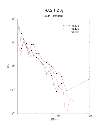
Figure 35: The $\xi(r)$ correlation function computed in the VL samples of IRAS $1.2Jy$ south (S). The amplitude of $\xi(r)$ shows a dependence on the sample size, even if the signal is rather noisy.

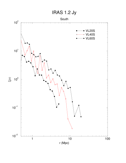
Figure 36: The $\xi(r)$ correlation function computed from the $\Gamma(r)$ function ($\xi(r)=\Gamma(r)/<n>-1$) in the VL samples of IRAS $1.2Jy$ south (S). The amplitude of $\xi(r)$ shows a clear dependence on the sample size.

In Fig.35 we show the behavior of $\xi(r)$ computed with the standard method, while in Fig.36 we show the $\xi(r)$ computed in different VL samples from the $\Gamma(r)$ function ($\xi(r)=\Gamma(r)/<n>-1$). While in the letter case a clear dependence of $r_{0}$ on the sample size is shown ($r_{0}\approx 8h^{-1}Mpc$ in the case of VL60). In the former case this dependence, although still present, is more noisy. This is probably due to the treatment of the boundary conditions (Sec.2.1.2.).

3.2 Analysis of clusters catalogs

With respect to the galaxy catalogs, cluster surveys offer the possibility to study the large scale structure of matter distribution in volumes much larger, reaching depths beyond $z\approx 0.2$ and extending all over the sky. Using clusters, one can trace matter distribution with a lower number of objects with respect to the galaxies, in the same volume. For example, in the northern hemisphere we know $\approx 10^{6}$ galaxies up to $z\approx 0.15$ which correspond to $\approx 500$ rich clusters. However the problem of cluster catalogs is their incompleteness, since clusters are identified as density enhancements in galaxy angular surveys and their distance is usually determined through the redshift of one or two galaxy members. It is clear, in fact, that only the measurements of every clusters (and member galaxies) allow us to construct truly VL samples. Moreover, as we show in what follows, there is a strong arbitrariness in the definition of a cluster: such an arbitrariness can be avoided by using the methods of modern statistical mechanics.

Cluster distribution shows large scale inhomogeneities and huge voids. Tully [70, 71] by investigating the spatial distribution of Abell and ACO catalog of clusters up to $300h^{-1}Mpc$, stressed that there are structures on a scale of $0.1c$ lying in the plane of the Local Supercluster. Galaxies clump in clusters and clusters in superclusters with extensions comparable to the largest scales of current samples. An analogous study on cluster distribution has been performed by Einasto et al.[72]. Their catalog of superclusters shows the presence of correlated structures with extension ranging from few $Mpc$ to $150h^{-1}Mpc$. Very similar results have been obtained by other compilations of Supercluster catalogs [22, 73, 74, 75].

Natural complementary aspect of presence of large structures is the presence of voids. Several authors [22, 73, 76, 72] have investigated the shape and the dimension of voids determined by rich clusters and superclusters. The dimension of a void can be defined as diameter of empty sphere containing no clusters. Clearly also for the voids there is an arbitrariness, because one can consider only spherical voids or ellipsoidal voids and so on. In particular, Einasto et al.[72] found that in their cluster sample (up to $z\approx 0.1$), the mean radius of voids is $50h^{-1}Mpc$. However, naturally, voids have elongated shapes and in one dimension they can exceed this value. These authors observe in fact a giant void which can exceed $300h^{-1}Mpc$ of length. A more detailed study on a single void, is performed by Lindner et al.[77], which have investigated the distribution of galaxies in and around the closest one, the Northern Local Void. The authors found that the dimension of the voids depends on the objects which have been used to defined them: voids defined by clusters are larger than galaxy defined voids, which are larger than faint galaxy defined voids. Search of extremely faint dwarf galaxies in voids has given, up to now, negative results [77] so that voids are real and not due to observational incompleteness. Moreover one observes an increased void size with sample depth, that may correspond to a self similarity in the distribution of voids [78].

As for galaxy distribution, the observations of large scale structures like superclusters and voids, which extends up to the limits of the samples investigated, clearly make questionable the existence of the average density. Usually, the presence of inhomogeneities on the scale of sample analyzed is interpreted as incompleteness of the samples themselves. However, up to now, better and more extensive observations have confirmed the reality of these structures, making the observed agglomeration sharper and not filling the voids.

For cluster distributions, the $\xi(r)$ function is a power law (Sec.2) $\xi(r)\approx(r_{0}/r)^{\gamma}$; both the exponent and the amplitude $r_{0}$ are uncertain. The exponent $\gamma$ generally appears consistent with the value $1.8$ observed for galaxy correlation function. In general high values for $r_{0}$ ($20\div 25h^{-1}Mpc$) are obtained for samples which contain the richer Abell/ACO clusters [22, 79, 80, 81, 82, 74] but some authors claim that these high values are overestimates, produced by systematic biases present in the Abell/ACO catalog [83, 84, 85, 86, 87]. When one corrects for these biases, a lower $r_{0}\approx 14h^{-1}Mpc$ is obtained. Lower values of $r_{0}$ ($13\div 15h^{-1}Mpc$) are obtained also from the analysis of automated cluster catalogs (APM, EDCC) and from the cluster catalogs selected from $X-ray$ galaxy survey, [88, 89, 90, 91, 92, 94, 95, 97]. In conclusion, for the samples analyzed so far we find that $14h^{-1}Mpc\mathrel{\hbox to0.0pt{\lower 3.0pt\hbox{$\mathchar 536\relax$}\hss}\raise 2.0pt\hbox{$\mathchar 316\relax$}}r_{0}\mathrel{\hbox to0.0pt{\lower 3.0pt\hbox{$\mathchar 536\relax$}\hss}\raise 2.0pt\hbox{$\mathchar 316\relax$}}25h^{-1}Mpc$.

Clusters are then found to be more aggregate than galaxies, for which $r_{0}$ is $\approx 5h^{-1}Mpc$. This mismatch between galaxy and cluster correlations is another puzzling feature of the usual analysis; clusters, in fact, are made by galaxies and many of these are included in the galaxy catalogs for which the correlation length $\approx 5h^{-1}\>Mpc$ was derived. It is therefore necessary to assume that cluster galaxies have fundamental differences with respect to the galaxies not belonging to a cluster. This concept has given rise to the so-called richness clustering relation [96, 22, 80, 98] according to which, objects with different mass or morphology would segregate from each other and give rise to different correlation properties, i.e. $r_{0i}\approx 0.4<n>^{-1/3}_{i}$ where the index $i$ refers to the system being considered, and $<n>_{i}$ is its mean spatial density. This hypothesis has been applied to explain the increase of $r_{0}$ going from APM and $X-ray$ less rich clusters to the Abell more rich clusters. As pointed out from Coleman & Pietronero [2] this preposition leads eventually to the paradox that every object is slightly different from any other and form, by its own, a morphological class, making totally meaningless the concept of correlation between galaxies. Szalay and Schramm [99] have interpreted the scaling of $r_{0}$ as signature of scale invariance properties of the distribution. This interpretation is inconsistent, since for self similar distributions, $r_{0}$ is proportional to $R_{eff}$, where $R_{eff}$ is the effective sample radius, and not to $<n>^{-1/3}$ (Sec.2).

In the following we present results of the statistical analysis on various samples of Abell and ACO clusters [100] The study of the spatial distribution of clusters requires a complete clusters sample covering a large volume. There are many available extensive catalogs of clusters from which one may try to extract complete subsamples. Here we present the analyses of several subsamples extracted from Abell and ACO catalogs.

From Abell catalog we have analyzed the Postman sample [74] that consists of 351 clusters with the tenth ranked galaxy magnitude ($m_{10}$)$\leq 16.5$, and it includes all such clusters which lie north of $\delta=-27^{\circ}30^{\prime}$. The typical redshift of a cluster with $m_{10}\leq 16.5$ is $z\approx 0.09$. To this redshift, incompleteness in the Abell catalog is considered insignificant [74]. About half of clusters have the redshifts based on at least three independent galaxy spectra; $25\%$ of the clusters have redshift determined from a single spectrum and $25\%$ from two galaxy spectra. Postman et al.[74] have defined a so called statistical subsample, which consist of 208 clusters with $z\leq 0.08$ and $|b|\geq 30^{\circ}$. This subsample has been shown to be minimally affected by selection biases. Then we have considered also the Bachall & Soneira [22] sample (BS83 hereafter) that includes 104 clusters of distance class $D\leq 4$ ($z\mathrel{\hbox to0.0pt{\lower 3.0pt\hbox{$\mathchar 536\relax$}\hss}\raise 2.0pt\hbox{$\mathchar 316\relax$}}1$), richness class $R\geq 1$, located at high galactic latitude ($|b|\geq 30^{\circ}$)

From the ACO catalog [101] we have selected all the clusters with measured redshift in according to the following constraints: $m_{10}\leq 16.4,b\leq-20^{\circ},\delta\leq-17^{\circ}$. This sample contains 139 clusters up to the limiting distance of $\approx 930h^{-1}Mpc$.

The completeness of the samples is usually estimated from the behavior of the clusters density as function redshift. As shown in Fig.37

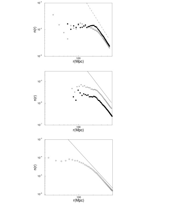
Figure 37: The radial density $n(r)$ from the vertex for a) Abell catalog Postman sample, north (diamonds) and south (filled circles) b) Abell catalog BS83 sample north (diamonds) and south (filled circles) c) ACO catalog sample (empty circles). the radial density shows large fluctuations, followed by a $r^{-3}$ decay due to the incompleteness of the samples.

the density, in almost every sample, presents large fluctuations followed by a power law decay as $\sim r^{-3}$. At closer distances the density is fluctuating because of the weak statistics in the samples, while at larger distances the sample is incomplete, i.e. the number of clusters is almost constant and the density decrease as $V^{-1}\sim r^{-3}$.

If one compute the radial density in bins, one obtains larger fluctuations, because this is a differential quantity while the integral density is much more smooth. Usually the fluctuating behavior of the density up to $z\mathrel{\hbox to0.0pt{\lower 3.0pt\hbox{$\mathchar 536\relax$}\hss}\raise 2.0pt\hbox{$\mathchar 316\relax$}}0.1$ is interpreted as a flat one, i.e. the density of the sample is considered to be constant and the distribution homogeneous; consequently the sample is considered complete and homogeneous up to this distance and incomplete beyond. At this regard, we note that up to the beginning of the incompleteness region, all the samples contain few clusters. The sparsest is the BS83 sample: the northern galactic part contains 53 clusters up to $230h^{-1}Mpc$ and the southern part 24. The Postman sample contains 120 clusters up to $z\approx 0.08$ in the northern part and 88 in the southern one. The ACO sample 91 up to the $150h^{-1}Mpc$.

The study of cluster spatial properties requires an almost complete sample; then it is necessary to exclude the incompleteness region. In the standard approach, one way to avoid such a problem is to correct the incompleteness by assuming an homogeneous distribution of clusters up to the sample limits. The observed distribution in the redshift space is then weighted with a selection function $p(z)$, that is the ratio between the observed counts of clusters in the volume $dV(z)$ at redshift $z$ and those expected from an homogeneous distribution. In our analysis, we want to avoid any assumption on the distribution itself and for this reason we limit our analysis up to a depth corresponding to the beginning of the incompleteness region, without correcting by means of any selection function.

Another selection effect exists, and it regards the observed depletion of the surface mean density of clusters at low galactic latitude (to $|b|\mathrel{\hbox to0.0pt{\lower 3.0pt\hbox{$\mathchar 536\relax$}\hss}\raise 2.0pt\hbox{$\mathchar 316\relax$}}30^{\circ}$). This is probably due to obscuration and confusion with high-density regions of stars of our galaxy [80]. As in the case of redshift incompleteness, one way to overcome this incompleteness is to weight the observed distribution with a latitude selection function $P(b)$, that is the ratio between observed surface cluster density at latitude $b$ and the expected one from an homogeneous distribution. The normalization of this selection function is arbitrary, because it depends on the real density. Another way is to limit the sample to high galactic latitude region. We adopt this standard procedure (i.e. $|b|\geq 30^{\circ}$ for Abell catalog and $b<-20^{\circ}$ for ACO), that has no assumptions but the inconvenient to slightly limit the sample. For the Postman sample the limiting distance is $\approx 230h^{-1}Mpc$ corresponding to $z\leq 0.08$, for the BS83 sample we have the same limiting distance, while for ACO sample is $\approx 150h^{-1}Mpc$. All these limits have been estimated from the behavior of the radial density versus the distance.

We have studied the behavior of $\>\Gamma(r)$ and $\>\Gamma^{*}(r)$ in the samples of Tab.2. The results for the Postman statistical subsample is shown in Fig.38

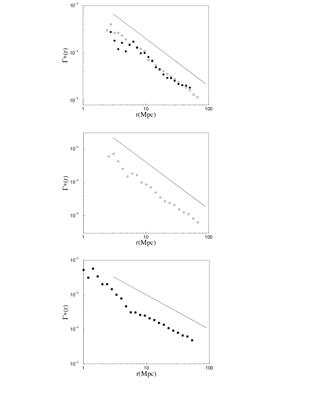
Figure 38: The behavior of the conditional density $\Gamma(r)$ and average conditional density $\Gamma^{*}(r)$ for a) Abell catalog Postman sample respectively north (diamonds) and south galactic parts (filled circles) b) Abell catalog BS83 sample north galactic part (diamonds), c) ACO catalog sample (filled circles). The conditional density has a power law behavior up to the radius of the largest sphere fully included in the sample. The reference line has slope $-\gamma=-1.0$.

separately for the southern galactic and northern galactic part. The southern galactic part has a smaller solid angle with respect the northern one and hence a smaller $R_{eff}$. A well defined power law behavior is detected up to the sample limit without any tendency towards homogenization. The codimension is, with good accuracy $\gamma=3-D\approx 1.0\pm 0.2$ so that $\>D\approx 2.0\pm 0.2$ up $\approx 70h^{-1}Mpc$ for the northern part and up to $\approx 50h^{-1}Mpc$ for the southern one. This result agrees well with the BS83 sample for the northern galactic part, where $D\approx 1.7\pm 0.2$ up to $r\approx 70h^{-1}Mpc$ (Fig.38). We have not reported the analysis for the BS83 southern galactic part, because it gives a very noisy result, due to the very weak statistics of the sample. The weaker statistics of the BS83 sample with respect to Postman’s one is also the reason for the small difference in the estimate of the fractal dimension $D$ of the two samples. The exponent $\gamma$ has a lower value with respect to the standard determination, and this is due to the fact that usually $\gamma$ has been estimated by the $\xi(r)$ analysis that has the problems discussed in Sec.2.

The results from the ACO sample are shown in the Fig.38. The $\Gamma(r)$ is a power law with exponent $D\sim 2.0\pm 0.1$ up to $\approx 50h^{-1}Mpc$. The fluctuations at $r<10h^{-1}Mpc$ are due to the fact that, at these distances, we are below the minimum average distance between nearest clusters in the sample ($\approx 15h^{-1}Mpc$ for Postman and BS83 and $\approx 8h^{-1}Mpc$ for ACO sample), as we have discussed in Sec.2.1.2. Hence we can interpret these fluctuations as a finite size effect due to a systematic depletion of points at these distances. In the correct regime, at distances $>10h^{-1}Mpc$, where the samples become statistically robust, the slope of $\Gamma(r)$ is almost the same for the Postman and ACO samples and, with a slight difference because the poor statistics, for the BS83 sample.

All the samples investigated so far have consistent statistical properties, i.e. they show a clear behavior of the correlation function. Note that long range correlations (fractal) can be only destroyed by incompleteness, but not produced by it. Hence the samples show well defined statistical properties, i.e. they are statistically fair samples; the results of the analysis is that they are not homogeneous samples, but, on the contrary, fractal.

We have studied the $\>\xi(r)$ in our cluster samples. In Fig.39

Figure 39: Upper part: Postman sample (north) (filled circles) Bottom part: Postman sample (south) (filled circles) and ACO (diamonds). The reference line is the functional form of $\xi(r)$ for a fractal with $\gamma\approx 1$

we have reported the $\xi(r)$ for the Postman sample (north and south) and for the ACO sample. We have fitted the experimental points with the functional form given by the fractal prediction (Sec.2.3). We found that $\>\gamma\approx 1$ for the all analyzed samples. The corresponding $r_{0}$ are reported in the Tab.2; for the Postman northern sample we found $r_{0}\approx 26\pm 2$ and for BS83 sample $r_{0}\approx 27\pm 2$. These two samples have the same $r_{0}$ because they have the same $R_{eff}$.

Sample	N	$\Omega$	$<n>$	$d_{lim}$	$R_{eff}$	$r_{0}$
		$sr$	$h^{3}Mpc^{-3}$	$(h^{-1}Mpc)$	$(h^{-1}Mpc)$	$(h^{-1}Mpc)$
BS83 N	$53$	$3.1$	$4.2\cdot 10^{-6}$	$230$	$70$	$27\pm 2$
Postman N	$120$	$3.1$	$9.5\cdot 10^{-6}$	$230$	$70$	$26\pm 2$
Postman S	$88$	$1.7$	$1.3\cdot 10^{-5}$	$230$	$53$	$17\pm 2$
ACO	$91$	$2.2$	$3.7\cdot 10^{-5}$	$150$	$50$	$17\pm 1$

Table 2: Features of the various samples analyzed; column I: the catalog from which the sample has been extracted; column II: number of clusters in the sample; column III: solid angle of the sample; column IV: density of the sample; column V: sample extension; column VI: radius of the maximum sphere fully included; column VII: the correlation length; column VIII: the mean separation

Same conclusions hold for the other two samples: Postman South and ACO. Both of them have $R_{eff}$ ($\approx 50h^{-1}Mpc$) and the same $r_{0}$ ($\approx 17h^{-1}Mpc$). In conclusion $r_{0}$ is simply a fraction of the sample size $R_{eff}$, without any real physical meaning.

In summary, the statistical analysis, performed without any a priori assumptions, shows that Abell samples have scale invariant properties with fractal dimension $D\approx 2$ up to $\approx 70h^{-1}Mpc$, while ACO sample up to $\approx 50h^{-1}Mpc$. The different limiting distance of the analysis in the various samples corresponds to the radius of the greatest sphere fully included in the sample. No tendency towards homogenization is detected within the sample limits. The so-called correlation length $r_{0}$ derived from the $\xi(r)$ analysis, is simply proportional to the sample size $R_{eff}$ and then, it is meaningless in relation with the correlation properties of the system.

The mismatch between galaxy and cluster correlation, i.e. the different correlation length for galaxies and clusters, is just due to the mathematical inconsistency of the use of $\xi(r)$ and the correct analysis, in terms of $\Gamma(r)$ and $\Gamma^{*}(r)$, show that cluster correlations are just the continuation at larger scales of galaxy correlations. We conclude that galaxies and clusters are two different representations of the same self similar structure. Our conclusion is therefore that galaxy clusters extend the correlations of galaxies to deeper depth; catalogs of clusters are deeper because clusters are more luminous than galaxies. To this end clusters distribution represents a coarse grained representation of galaxies, i.e. it is the same self-similar distribution, but sampled with a larger scale resolution. In other words, we consider a cluster of galaxies as a single object without distinguish the structure in it. Hence, we can study the clusters distribution simply performing a coarse graining on galaxy distribution. Usually clusters are instead identified with some criteria, which are different according to different observers. On the contrary, in this way, we can make the analysis independently on the definition of cluster or supercluster etc. The price that one has to pay is however the availability of a complete galaxy sample. Same considerations hold, of course, for the voids distribution: the void distribution is, in fact, just the complement of matter one.

3.3 Scaling of $r_{0}$ and luminosity segregation

A possible explanation of the shift of $r_{0}$ with sample size is based on the luminosity segregation phenomenon [49, 38]. We briefly illustrate this approach. The fact that the giant galaxies are more clustered than the dwarf ones, i.e. that they are located in the peaks of the density field, has given rise to the proposition that larger objects may correlate up to larger length scales and that the amplitude of $\>\xi(r)$ is larger for giants than for dwarfs one. The deeper VL samples contain galaxies which are in average brighter than those in the VL samples with smaller depths. As the brighter galaxies should have a larger correlation length the shift of $r_{0}$ in different samples can be related, at least partially, with the phenomenon of luminosity segregation.

To show that this is not the case for the PP survey (for example) and that, on the contrary, the shift of $\>r_{0}$ is simply due to the fractal nature of the galaxy distribution, we have performed the following test. We consider a sample of galaxies with apparent magnitude lower $14.5$ (hereafter PP14.5). It is evident that the VL sample with the same absolute magnitude limit $M_{lim}$ have different limiting depth $\>d_{lim}$ for the two catalogs according to the formula

$$d_{lim}=10^{0.2\cdot(m_{lim}-M_{lim}-25)}$$ (66)

where $m_{lim}$ is $15.5$ or $14.5$. Then we construct some VL subsamples for the PP14.5 catalog whose characteristics are reported in the Appendix. For these VL samples we have done the same analysis as for the whole catalog PP, and the behavior of $r_{0}$ as a function of $R_{eff}$ is again well fitted by the fractal prediction as for the whole catalog PP.

In Fig.40 we compare the values of $r_{0}$ obtained in VL samples

Figure 40: The ”Characteristic length scale” $r_{0}$ ($\xi(r_{0})\equiv 1$) plotted as a function of the absolute magnitude limit $M_{lim}$ for PP (crosses) and PP14.5 (squares). To test the luminosity segregation hypothesis, one should find that $r_{0}$ is the same for sample with same the $M_{lim}$. It is clear that there is no agreement between these values. On the contrary, the fractal nature of galaxy distribution explains completely the shift of $r_{0}$ with sample size. Hence the hypothesis of luminosity segregation has no experimental support.

of PP and PP14.5 with the same absolute magnitude limit $M_{lim}$. For example the subsample VL70(b) (we refer with (b) to the 14.5 sample) has the same absolute magnitude limit of the sample VL110 of PP ($M_{lim}=-19.78$). Hence these two samples contain galaxies with the same average absolute magnitude (Appendix). If the shift of $r_{0}$ is due to the luminosity segregation effect we should not find any difference for $\>r_{0}$. As shown in Fig.40 this is not the case. In fact, for VL70(b) we find that $r_{0}\approx 5h^{-1}Mpc$ while for VL110 $\>r_{0}\approx 8h^{-1}Mpc$. On the contrary, if we consider the sample depth dependence of $\>r_{0}$ we find that for VL70(b) $R_{s}\sim 15h^{-1}Mpc$ that is the same limiting depth of the subsample VL70 for which $\>r_{0}\approx 5h^{-1}Mpc$.

Our conclusion is that luminosity segregation cannot be the physical effect of the shift of $\>r_{0}$ with sample size and that, on the contrary, the linear dependence of $\>r_{0}$ on depth is naturally described by the fractal nature of the galaxy distribution. The observation that the giant galaxies are more clustered than the dwarf ones, i.e. that the massive elliptical galaxies lie in the peaks of the density field, is a consequence of the self-similar behavior of the whole matter distribution (Sec.8). The increasing of the correlation length of the $\xi(r)$ has nothing to do with this effect [2]. As far as a clear cut-off towards homogeneity has not been clearly identified, quantities like $r_{0}$ are meaningless.

Finally we stress the conceptual problems of the interpretation of the scaling of $r_{0}$ by the luminosity segregation phenomenon. Suppose we have two kind of galaxies of different masses, one of type $A$ and the other of type $B$. Suppose for simplicity that the mass of the galaxies of type $A$ is twice that of the $B$. The proposition ”galaxies of different luminosities (masses) correlate in different ways” implies that the gravitational interaction is able to distinguish between a situation in which there is, in a certain place, a galaxy of type $A$ or two galaxies of type $B$ placed nearby. This is a paradox, as the gravitational interaction is due the sum of all the masses. We can go farther by showing the inconsistency of the proposition ”galaxies of different luminosities have a different correlation length”. Suppose that the galaxies of type $A$ have a smaller correlation length than that of the galaxies of type $B$ (Fig.41).

Figure 41: Luminosity segregation: in this example we have two kind of objects. Galaxies $A$ have power law correlation up to $\lambda(A)$ and then they became homogeneous. Galaxies $B$ have the same behavior, but up to $\lambda(B)>\lambda(A)$. In this case the voids of $B$ galaxies should be full of galaxies $A$.

This means that the galaxies of type $B$ are still correlated (in terms of the conditional density) when the galaxies of type $A$ are homogeneously distributed. This means that the galaxies of type $A$ should fill the voids of galaxies of type $B$. This is not the case, as the voids are empty of all types of galaxies, and it seems that the large scale structures distribution is independent on the galaxy morphological types (Sec.8). We refer to Sec.4 for a discussion about several additional tests on luminosity segregation we have performed by the power spectrum analysis.

3.4 Tests on the treatment of boundary conditions

In order to test the usual receipt of treatment of boundary conditions [18], we have computed the conditional density applying the standard method. In this case one does not limit the analysis up to the radius of the maximum sphere fully contained in the sample volume $R_{eff}$. Rather one computes the correlation function up to the maximum distance between two galaxies in the sample. In particular the correlations are derived from pair counts in redshift space [49, 89] by using the estimator

$$1+\xi(r)=\frac{DD(r)}{DR(r)}\left(\frac{N_{R}}{N_{D}}\right)$$ (67)

where $DD(r)$ is the number of pair counts of galaxies at distance separation $r$, and $DR(r)$ is the number of pairs consisting of a galaxy and a randomly distributed point, chosen within the same catalog window, at distance separation $r$. $N_{R}$ and $N_{D}$ are the total number of points in the random and galaxy catalogs respectively. From Eq.67 one can easily computes the conditional density

$$\Gamma(r)=<n>(1+\xi(r))$$ (68)

where $<n>$ is the average density in the real sample.

We have computed Eq.67 in the case of an artificial fractal distribution, generated by the random $\beta$ model algorithm [30]. The artificial sample has the same geometry of the Perseus-Pisces survey (a part an arbitrary rescaling of distances, we have that $R_{eff}\approx 50h^{-1}Mpc$), and the distance of statistical validity is $R_{eff}\sim 30h^{-1}Mpc$. We show the results in Fig.42.

Figure 42: $\xi(r)+1$ for an artificial fractal computed by the standard method. The crossover towards homogenization is clearly spurious and due to the treatment of boundary conditions. The reference line has a slope $-\gamma=-1.1$

This sample shows well defined power law correlations up to $R_{eff}\sim 50h^{-1}Mpc$, with fractal dimension $D\approx 2$. At larger scales a clear crossover towards homogenization is shown. This is clearly spurious, because the sample is scale invariant by construction without any characteristic scale. We have done the same test in the real Perseus-Pisces sample, finding the same behavior (see Fig.43, that is in agreement with the results of [52]).

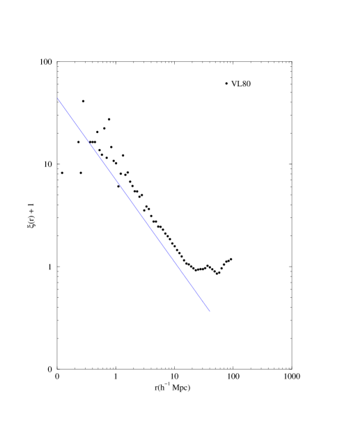
Figure 43: $\xi(r)+1$ for the volume limited sample VL80 of the Perseus-Pisces redshift survey, computed by the standard method. The crossover towards homogenization is spurious and due to the inappropriate way of treating the boundary conditions. The reference line has a slope $\gamma=-0.9$.

The reason why, by applying the standard procedure we find a flattening of the conditional density for distances larger than $R_{eff}$, is the following. Suppose that we are computing the average conditional density $\Gamma^{*}(r)$ for a sample limited by boundaries shown in Fig.44.

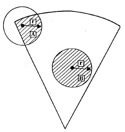
Figure 44: The inclusion of the point A in the statistics corresponds to an implicit assumption of homogeneity. It implies in fact that the smaller region around A included in the sample, and the larger region around B, both contribute to the average density at distance $r$, each with a weight given by its volume (From Coleman & Pietronero, 1992).

For a point B, the sphere centered on B and of radius $r$ is completely included in the sample, while this is not the case for the point A. The filled region around A corresponds therefore to an effective length scale that is actually shorter than $r$ and the inclusion of this point, even if properly weighted by its volume, in the statistics gives rise to an artificial homogenization of the sample. If the system has long range correlations, the mixing of regions of different sizes for the same nominal distance $r$ cannot be correct [2].

3.5 Tests on the conditional density stability versus errors in the apparent magnitude

Some authors (e.g. [19]) claimed that the long range correlations we detected can be due to systhematic selection effects in the data or to observational errors. To check that possible errors in the apparent magnitude do not affect seriously the behavior of $\Gamma(r)$ we have performed the following tests. We have changed the apparent magnitude of galaxies in the whole catalog by a random factor $\delta m$ with $\delta m=\pm 0.2,0.4,0.6,0.8$ and $1$. We find that the number of galaxies in the VL samples change from $5\%$ up to $15\%$ and that the amplitude and the slope of $\Gamma(r)$ are substantially stable and there are not any significant changes in their behavior. This is because $\Gamma(r)$ measures a global quantity that is very robust with respect to these possible errors.

In particular in Fig.45 we show the behavior of the conditional density in the CfA1 catalog limited at $m_{lim}=14.5$, having added a random error up to $\delta=\pm 0.5$ to each galaxy in the survey. The correlation properties are not substantially affected by such an error.

Figure 45: Behavior of the average conditional density in the CfA1 catalog limited at $m_{lim}=14.5$, having added a random error up to $\delta=\pm 0.5$ to each galaxy in the survey. The correlation properties are not substantially affected by such an error.

Moreover we have cut the catalog at $m_{lim}=14$ and we have added again a random error of $\delta=0.5$ to the apparent magnitude. In such a way we have a symmetric situation for the galaxies brighter and fainter than $14$. In Fig.46 we show the result of such a test.

Figure 46: Behavior of the average conditional density in the CfA1 catalog limited at $m_{lim}=14.0$, having added a random error up to $\delta=\pm 0.5$ to each galaxy in the survey. The correlation properties are again stable with respect to these eventual effects

We have done the same tests in the Perseus-Pisces catalog and we show in Fig.47 and Fig.48 the results.

Figure 47: Behavior of the average conditional density in the Perseus-Pisces catalog limited at $m_{lim}=15.5$, having added a random error up to $\delta=\pm 0.2$ to each galaxy in the survey. The correlation properties are not substantially affected by such an error

Figure 48: Behavior of the average conditional density in the Perseus-Pisces catalog limited at $m_{lim}=15.0$, having added a random error up to $\delta=\pm 0.5$ to each galaxy in the survey. The correlation properties are again stable with respect to these eventual effects

Moreover to check that the eventual incompleteness of the catalog for $m\rightarrow m_{lim}=15.5$ do not affect $\Gamma(r)$ we have done another test. We have changed again the apparent magnitude of galaxies, but with a probability density given by $P(m)\sim 10^{\alpha m}$ where $\alpha\sim 0.4\div 0.6$ is the number counts exponent (Sec.7). Even in this case neither the amplitude nor the slope of $\Gamma(r)$ are changed by this eventual incompleteness. These tests confirm that the results shown in Fig.16 are genuine features of the galaxy distribution.

We stress and the end of this section, that a fractal distribution has a very strong feature: it shows power law correlations up to the sample depth. Such correlations cannot be due neither by an inhomogeneous sampling of an homogeneous distribution, nor by some selection effects that may occur in the observations. Namely, suppose that a certain kind of sampling reduces the number of galaxies as a function of distance [102]. Such an effect in no way can lead to long range correlations, because when one computes $\Gamma(r)$, one makes an average over all the points inside the survey. Of course such a selection effect may bias the determination of the space density determined from only one point, i.e. the radial density as we discuss in Sec.6.5.

4 Power spectrum of galaxy distributions

In a series of papers [103, 104, 59, 60] we have studied the problems of the determination of the power spectrum in galaxy redshift surveys. Here we briefly review our main results, and we present several analyses on real redshift surveys .

First of all we stress an important conceptual point that makes the determination of the power spectrum ambiguous, in the case of fractal structures. In fact, if we have a fractal distribution that has correlation function that decays as a power law $\Gamma(r)\sim r^{D-3}$, its Fourier conjugate is a power law too: $\Pi(k)\sim k^{-D}$. However, there is an additional problem that is usually neglected. Namely, if we have a power spectrum which decays as power law of the wavenumber, then it is not needed that the real space distribution is fractal. The key point is that the existence of correlated structures in real space implies that the phases of the different modes of the power spectrum are not randomly distributed, but are correlated as well. This fact shows the conceptual problem in the determining the power spectrum: in fact, in general it is possible to compute the behavior of the amplitude of the power spectrum at various modes, but the eventual phases correlation, at different modes, is very difficult to study. All the determinations of the power spectrum in literature refers to the shape of power spectrum, rather than to the distribution of phases. Hence the most effective way to study a fractal structure is the real space correlation analysis.

In the following we stress the technical problems of the standard determination of the power spectrum and we clarify the correct interpretation of the results. The problems are strictly related to those of $\xi(r)$, namely that this function is not a power law for a fractal structure and its amplitude depends on the sample size. We introduce the correct quantity that should be computed in order to perform an analysis without a priori assumptions, that is the Fourier conjugate of the conditional density.

4.1 Power spectrum analysis of galaxy distribution

Essentially all the currently elaborated models of galaxy formation (e.g [3]) assume large scale homogeneity and predict that the galaxy power spectrum (hereafter PS), which is the PS of the density contrast, decreases both toward small scales and toward large scales, with a turnaround somewhere in the middle, at a scale $\lambda_{f}$ that can be taken as separating “small” from “large” scales. Because of the homogeneity assumption, the PS amplitude should be independent on the survey scale, any residual variation being attributed to luminosity bias (or to the fact that the survey scale has not yet reached the homogeneity scale). However, the crucial clue to this picture, the firm determination of the scale $\lambda_{f}$, is still missing, although some surveys do indeed produce a turnaround scale around 100 $h^{-1}Mpc$ [105, 106]. Recently, the CfA2 survey analyzed by [38] (hereafter PVGH) (and confirmed by SSRS2 [37] - hereafter DVGHP), showed a $n=-2$ slope up to $\sim 30h^{-1}Mpc$, a milder $n\approx-1$ slope up to 200 $h^{-1}Mpc$, and some tentative indication of flattening on even larger scales. PVGH also find that deeper subsamples have higher power amplitude, i.e. that the amplitude scales with the sample depth.

In the following we argue that both features, bending and scaling, are a manifestation of the finiteness of the survey volume, and that they cannot be interpreted as the convergence to homogeneity, nor to a PS flattening. The systematic effect of the survey finite size is in fact to suppress power at large scale, mimicking a real flattening. Clearly, this effect occurs whenever galaxies have not a correlation scale much larger than the survey size, and it has often been studied in the context of standard scenarios [107, 108]. We push this argument further, by showing that even a fractal distribution of matter, which never reaches homogeneity, shows a sharp flattening and then a turnaround. Such features are partially corrected, but not quite eliminated, when the correction proposed by [109] is applied to the data. We show also how the amplitude of the PS depends on the survey size as long as the system shows long-range correlations.

The standard PS (SPS) measures directly the contributions of different scales to the galaxy density contrast $\>\delta\rho/\rho$. It is clear that the density contrast, and all the quantities based on it, is meaningful only when one can define a constant density, i.e. reliably identify the sample density with the average density of all the Universe. In other words in the SPS analysis one assumes that the survey volume is large enough to contain a homogeneous sample. When this is not true, and we argue that is indeed an incorrect assumption in all the cases investigated so far, a false interpretation of the results may occur, since both the shape and the amplitude of the PS (or correlation function) depend on the survey size.

Let us recall the basic notation of the PS analysis. Following Peebles [25] we imagine that the Universe is periodic in a volume $\>V_{u}$, with $\>V_{u}$ much larger than the (presumed) maximum correlation length. The survey volume $V\in V_{u}$ contains $\>N$ galaxies at positions $\>\vec{r_{i}}$, and the galaxy density contrast is

$$\delta(\vec{r})=\frac{n(\vec{r})}{\hat{n}}-1$$ (69)

where it is assumed that exists a well defined constant density $\hat{n}$, obtained averaging over a sufficiently large scale. The density function $\>n(\vec{r})$ can be described by a sum of delta functions: $~{}n(\vec{r})=\sum_{i=1}^{N}\delta^{(3)}(\vec{r}-\vec{r_{i}})\,.~{}$ Expanding the density contrast in its Fourier components we have

$$\delta_{\vec{k}}=\frac{1}{N}\sum_{j\epsilon V}e^{i\vec{k}\vec{r_{j}}}-W(\vec{k})\,,$$ (70)

where

$$~{}W(\vec{k})=\frac{1}{V}\int_{V}d{\vec{r}}W(\vec{r})e^{i\vec{k}\vec{r}}\,~{}$$ (71)

is the Fourier transform of the survey window $W(\vec{r})$, defined to be unity inside the survey region, and zero outside. If $\xi(\vec{r})$ is the correlation function of the galaxies ($\xi(\vec{r})=<n(\vec{r})n(0)>/\hat{n}^{2}-1$), the true PS $\>P(\vec{k})$ is defined as the Fourier conjugate of the correlation function $\xi(r)$. Because of isotropy the PS can be simplified to

$$P(k)=4\pi\int\xi(r)\frac{\sin(kr)}{kr}r^{2}dr\,.$$ (72)

The variance of $\>\delta_{\vec{k}}$ is [25, 109, 110]

$$<|\delta_{\vec{k}}|^{2}>=\frac{1}{N}+\frac{1}{V}\tilde{P}(\vec{k})\,.$$ (73)

The first term is the usual additional shot noise term while the second is the true PS convoluted with a window function which describe the geometry of the sample (PVGH)

$$\tilde{P}(\vec{k})={V\over(2\pi)^{3}}\int<|\delta_{\vec{k^{\prime}}}|^{2}>|W(\vec{k}-\vec{k^{\prime}})|^{2}d^{3}\vec{k^{\prime}}\,.$$ (74)

$$\tilde{P}(\vec{k})=\int d\vec{k^{\prime}}P(\vec{k^{\prime}})F(\vec{k}-\vec{k^{\prime}})\,,$$ (75)

with

$$F(\vec{k}-\vec{k^{\prime}})=\frac{V}{(2\pi)^{3}}|W(\vec{k}-\vec{k^{\prime}})|^{2}\,.$$ (76)

We apply now this standard analysis to a fractal distribution. We recall the expression of the $\>\xi(r)$ in this case is (Sec.2):

$$\xi(r)=[(3-\gamma)/3](r/R_{s})^{-\gamma}-1\,,$$ (77)

where $\>\gamma=3-D$. A key point of our discussion is that that on scales larger that $R_{s}$ the $\xi(r)$ cannot be calculated without making assumptions on the distribution outside the sampling volume.

As we have already mentioned, in a fractal quantities like $\xi(r)$ are scale dependent: in particular both the amplitude and the shape of $\xi(r)$ depend the survey size. It is clear that the same kind of finite size effects are also present when computing the SPS, so that it is very dangerous to identify real physical features induced from the SPS analysis without first a firm determination of the homogeneity scale.

The SPS for a fractal distribution model described by Eq.77 inside a sphere of radius $R_{s}$ is

$$P(k)=\int^{R_{s}}_{0}4\pi\frac{\sin(kr)}{kr}\left[\frac{3-\gamma}{3}\left(\frac{r}{R_{s}}\right)^{-\gamma}-1\right]r^{2}dr=\frac{a_{k}(R_{s})R_{s}^{3-D}}{k^{D}}-\frac{b_{k}(R_{s})}{k^{3}}\,.$$ (78)

Notice that the integral has to be evaluated inside $R_{s}$ because we want to compare $P(k)$ with its estimate in a finite size spherical survey of scale $R_{s}$. In the general case, we must deconvolve the window contribution from $P(k)$; $R_{s}$ is then a characteristic window scale. Eq.78 shows the two scale-dependent features of the PS. First, the amplitude of the PS depends on the sample depth. Secondly, the shape of the PS is characterized by two scaling regimes: the first one, at high wavenumbers, is related to the fractal dimension of the distribution in real space, while the second one arises only because of the finiteness of the sample. In the case of $\>D=2$ in Eq.78 one has:

$$~{}a_{k}(R_{s})=\frac{4\pi}{3}(2+\cos(kR_{s}))\,$$ (79)

and

$$~{}b_{k}(R_{s})=4\pi\sin(kR_{s})\,.$$ (80)

The PS is then a power-law with exponent $\>-2$ at high wavenumbers, it flattens at low wavenumbers and reaches a maximum at $k\approx 4.3/R_{s}$, i.e. at a scale $\lambda\approx 1.45R_{s}$. The scale at which the transition occurs is thus related to the sample depth. In a real survey, things are complicated by the window function, so that the flattening (and the turnaround) scale can only be determined numerically (Fig.49).

Figure 49: Left panel: Standard PS $P(k)$ for an artificial fractal distribution. It rises as $\lambda^{D}$ ($\lambda=2\pi/k$) for small scales, it reaches a turnaround at $\lambda\approx 1.5R_{s}$ and then it declines to zero as $\lambda\to\infty$. Moreover the sample size dependence of the amplitude of the PS is shown. Right panel: The same of the previous case, but with PS of the density, $\Pi(k)$.

In practice, one averages the spectrum over $k$-shells of thickness $\Delta\leq 2\pi/R_{s}$:

$$P_{a}(k)={1\over k^{2}\Delta}\int_{k}^{k+\Delta}P(k^{\prime})k^{\prime 2}dk^{\prime}$$ (81)

For $D=2$ and for $\Delta=2\pi/R_{s}$ one has

$$P_{a}(k)=(8\pi R_{s}/3k^{2})[1+f(x)]\approx 8\pi R_{s}^{3}/3k^{2}$$ (82)

where $f(x)=3[Si(2\pi+x)-Si(x)]/4\pi\ll 1$ for $x>1$ (here $Si(x)$ is the SinIntegral function). Thus, in the case of a spherical survey, with $D=2$ and $\Delta=2\pi/R_{s}$, the fractal PS goes like the simple power law $k^{-2}$, and the turnaround feature is removed. For smaller $\Delta$, the turnaround at small $k$ appears also in the shell-averaged spectrum $P_{a}(k)$. We calculated numerically the PS for $D\not=2$, and we found that the generalization

$$P_{a}(k)\approx 8\pi R_{s}^{3-D}/3k^{D}$$ (83)

is accurate to better than 10% for $D$ in the range $(1.7,2.3)$.

However, in practice one has several complications. First, the survey in general is not spherical. This introduces a coupling with the survey window which is not easy to model analytically. For instance, we found that windows of small angular opening shift to smaller scales the PS turnaround. This is analogous to what happens with the correlation function of a fractal: when it is calculated in small angle surveys, the correlation length $r_{0}$ decreases. Second, the observations are in redshift space, rather than in real space. The peculiar velocities generally make steeper the PS slope (e.g. [110]) with respect to the real space. Third, in a fractal the intrinsically high level of fluctuations makes hard a precise comparison with the theory when the fractal under study is composed of a relatively small number of points. In view of these complications, we compare our results with the simple fractal-like trend

$$P(k)=AR_{s}^{3-D}k^{-D}\;.$$ (84)

4.2 Sample-size independent PS

As we have already discussed, the analysis of a distribution on scales at which homogeneity is not reached must avoid the normalization through the mean density, if the goal is to produce results which are not related to the sample size, and thus misleading. To this aim, now we consider the sample size-independent PS (SIPS) of the density $\>\rho(\vec{r})$, a quantity which gives an unambiguous information of the statistical properties of the system. We first recall the density correlation function (Sec.2)

$$G(\vec{r})=<\rho(\vec{x}+\vec{r})\rho(\vec{x})>=Br^{-(3-D)}\,,$$ (85)

where the last equality holds in the case of a fractal distribution with dimension D, and where B is a constant determined by the lower cut-offs of the distribution (Sec.2). Defining the SIPS as the Fourier conjugate of the correlation function $G(r)$,

$$\Pi(k)=4\pi\int G(r)\frac{\sin(kr)}{kr}r^{2}dr\,,$$ (86)

one obtains that in a finite spherical volume

$$\Pi(k)\sim B^{\prime}k^{-D}$$ (87)

(where $B^{\prime}=4\pi B(1-\cos(kR_{s}))$ if $D=2$) so that the SIPS is a single power law extending all over the system size, without amplitude scaling with the sample depth (except for $kR_{s}\ll 1$). Taking into account the window function, we can write the convolution of the SIPS with a window function in complete analogy to Eq.74. In analogy to the procedure above, we consider the Fourier transform of the density

$$\rho_{\vec{k}}=\frac{1}{V}\sum_{j\in V}e^{-i\vec{k}\vec{x_{j}}}\,,$$ (88)

and its variance

$$<|\rho_{\vec{k}}|^{2}>=\frac{1}{V}\tilde{\Pi}(\vec{k})+\frac{1}{N}\,,$$ (89)

where $\tilde{\Pi}(\vec{k})$ is the same as in Eq.74, with $<|\rho_{\vec{k^{\prime}}}|^{2}>$ instead of $<|\delta_{\vec{k^{\prime}}}|^{2}>$.

$$\tilde{\Pi}(\vec{k})=\int d\vec{k^{\prime}}\Pi(\vec{k^{\prime}})F(\vec{k}-\vec{k^{\prime}})\,.$$ (90)

4.3 Tests on artificial distributions

In order to study the finite size effects in the determinations of the PS, we have performed some tests on artificial distributions with a priori assigned properties [103]. We distribute the sample in a cubic volume $\>V_{u}$. We determine $P(k)$ ($\Pi(k)$) defined as the directionally averaged $\>P(\vec{k})$ ($\>\Pi(\vec{k})$). Following PVGH, the estimate of the noise-subtracted PS given in Eq. (74) for a strongly peaked window function is

$$P(\vec{k})=\left(<|\delta_{k}|^{2}>-\frac{1}{N}\right)\left(\sum_{\vec{k}}|W_{\vec{k}}|^{2}\right)^{-1}(1-|W_{\vec{k}}|^{2})^{-1}\,,$$ (91)

For the lowest wavenumbers the PS estimate Eq.91 is not acceptable, because then the window filter flattens sensibly (see e.g. PVGH). The factor $\>(1-|W_{\vec{k}}|^{2})^{-1}$ has been introduced by [109] as an analytical correction to the erroneous identification of the sample density with the population density. However, the correction itself rests on the assumption that the PS is flat on very large scales; in other words, it implies the flattening, which is just the feature we are testing for. PVGH actually correct their results by comparing them to the power spectra of $N$-body simulations; their conclusion is that the PS correction is a procedure reliable for wavelengths smaller than $\sim 200h^{-1}Mpc$.

We have generated $D\approx 2$ fractal distributions with the random $\>\beta$-model algorithm [30]. Then we have constructed artificial volume limited catalogs with roughly the same geometry of the CfA2 survey (our model contains no dynamics, so that we can think of our fractal set as lying in redshift space, as the CfA2 galaxies). We have computed the quantity $\>P(k)$ from Eq.91 averaging over 50 random observers (located on one of the particles) for each realization. In Fig.50

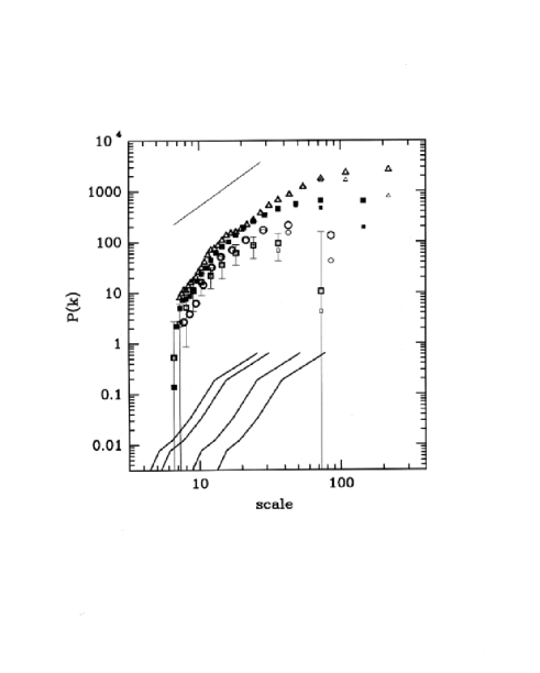
Figure 50: Top panel: Power spectrum for a fractal distribution with dimension $\>D=2$ vs. the scale $2\pi/k$ without the correction factor (filled squares) and with the correction factor (open triangles). Here and in what follows the error bars represent the scatter among the different observers of the same fractal. The upper set of points refer to a subsample of depth 60 cells, the lower set to a depth of 30 cells. The dashed lines are least squares linear fit to the data, at small scales (slope $D_{1}$ and amplitude $10^{A}$) and at large scales (slope $D_{2}$). At low wavenumbers there is a well defined power law behavior with exponent $\>D_{1}\approx 2$. The flattening at high wavenumber is spurious. In the bottom panel it is shown the window function. (From Sylos Labini & Amendola, 1996).

it is shown the $\>P(k)$ vs. the scale $2\pi/k$ with and without the correction factor, for some different survey scales $R_{s}$, together with the angle-averaged window PS $\>|W_{k}|^{2}$. The slope of the PS at high wavenumbers is $\>\approx-D$ in agreement with Eq.78. As anticipated, the flattening at low wavenumbers is here completely spurious, i.e. it is due to the finite volume effects on the statistical analysis performed. In fact, comparing the PS at the various sample scales, one finds the turnaround of the PS always occurs near the boundary of the sample. The turnaround scale roughly follows the relation $\lambda=1.5R_{s}$ as predicted previously. Notice that the PS starts flattening before the window spectrum flattens; as in PVGH, the change in slope occurs for $|W_{k}|^{2}<0.2$, value that they assumed as preliminary condition for the estimate Eq.91 to be valid. The amplitude of the PS scales according to Eq.78. In Fig.51 it is shown the behavior of $\>\Pi(k)$

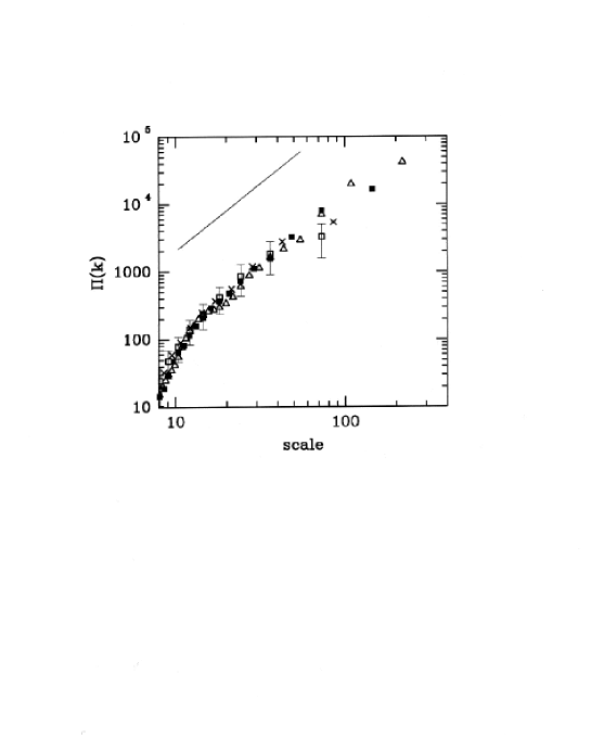
Figure 51: The scale-independent PS for the same fractal and the same4.2 scales as in Fig.50. Now the spectrum is a single power law, up to the very few large scales, at which the flattening of the window PS make the spectrum estimator invalid. The amplitude of the spectrum is now constant (inside the errors). (From Sylos Labini & Amendola, 1996).

computed from Eq.91 with $<|\rho_{k}|^{2}>$ in place of $<|\delta_{k}|^{2}>$ and without the Peacock-Nicholson correction: as predicted, its amplitude does not scale with the sample size and it is characterized by a single power law behavior, up to very large scales (where the two terms in the coefficient $A^{\prime}$ of $\Pi(k)$ are comparable) .

4.4 CfA2 and SSRS2

Let us summarize the results of PVGH on CfA2, by comparing them with the analysis of the PS for a fractal distribution: i) for $\>k\geq 0.25$ ($\>\lambda\leq 25h^{-1}$ Mpc) the PS is very close to a power law with slope $\>n=-2.1$. In our view, this is the behavior at high wavenumbers connected with the real fractal dimension. ii) For $\>0.05\leq k\leq 0.2$ ($120h^{-1}Mpc>\lambda>30h^{-1}Mpc$) the spectrum is less steep, with a slope about $\>-1.1$. This bending is, in our view, solely due to the finite size of the sample. iii) The amplitude of the volume limited subsample CfA2-130 PS is $\>\sim 40\%$ larger than for CfA2-101. This linear scaling of the amplitude can be understood again considering that the sample is fractal with $\>D=2$. It is important to notice that this trend is qualitatively confirmed by the results of Peacock & Nicholson [109] who find a higher PS amplitude for a deep radio-galaxy survey. On the contrary the PVGH explain this fact considering the dependence of galaxy clustering on luminosity: brighter galaxies correlate more than fainter ones. They support this interpretation with the observation that brighter galaxies tend to avoid underdense regions; they also analyze separately two subsets of the same volume-limited sample of CfA2, one brighter than the other, and find in some cases a luminosity-amplitude correlation. However, PVGH do not detect such a luminosity segregation for the two largest subsamples, CfA2-101 and CfA2-130, to which we are comparing here.

In Fig.52

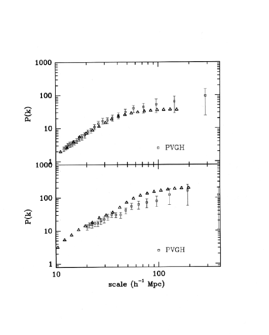
Figure 52: Comparison of the power spectra of fractal distribution (triangles) with the CfA2 survey (squares). In the top panel we plot the PS of the subsample CfA2-130 (PVGH) along with the PS of our artificial fractal distribution (without the error bars for clarity). In the bottom panel, we plot CfA2-101 (PVGH) and a subsample of the same fractal as above, with a correspondingly scaled depth (from Sylos Labini & Amendola, 1996).

we compare directly the PS of our artificial catalogs with the PS of the CfA2 subsamples obtained generating two volume limited subsamples at 130 and 101 $h^{-1}Mpc$ (PVGH). The physical scale has been computed matching the CfA2-101 galaxy average density. Both the shapes and the amplitudes are compatible with a fractal distribution: for CfA2-101 the agreement is excellent; for CfA2-130 the two curves are compatible inside the errors.

It seems therefore that the amplitude scaling at these scales can be entirely attributed to the fractal scaling. Our conclusion is then that the fractal nature of the galaxy distribution can explain, to the scales surveyed in the CfA2 survey, the shift of the amplitude of the PS.

4.5 LEDA

The LEDA database has been described elsewhere (see Sec.3 and the Appendix). Here we only present the subsamples we have analyzed. We extract from LEDA two magnitude limited samples, one at $m_{lim}=15.5$ and the other at $m_{lim}=16$. The first cut is to reduce it to the CfA-North boundaries (R.A. $8^{h}<\alpha<17^{h}$, declination $8.5^{0}<\delta<44.5^{0}$, with a further cut to reduce galactic obscuration, see PVGH), and is denoted as LEDA-CfA sample. This sample contains 4593 galaxies in an angular area of 1.1 sr, amounting to a completeness level of 70% (CfA2 North contains in this region 6478 galaxies, see PVGH). The LEDA-CfA sample is then cut into several volume-limited subsamples, at depths 60,78,101 and 130 $h^{-1}Mpc$, to reproduce the PVGH results, and at various average magnitudes, as summarized in Tab.3. The second sample, to be denoted as LEDA16, contains galaxies with $m<16$, and is cut to $b>20^{0}$ to reduce galactic obscuration. LEDA16 contains 12801 galaxies for an angular area of $4.13sr$, and is estimated to be complete to 60%.

SAMPLE	$M_{1}$	$M_{2}$	numb.
			of gal.
r60m187	-19	-18.5	330
r60m198	-	-19.28	301
r60m193	-19.8	-18.9	360
r78m193	-19.5	-19.1	492
r78m198	-20.15	-19.55	431
r78m202	-	-19.75	445
r100m198	-19.45	-19.7	414
r100m202	-20.5	-19.98	428
r100m205	-	-20.13	431
r130m205	-20.8	-20.3	371
r130m208	-	-20.45	343

Table 3: The VL subsamples of LEDA-CfA. $M_{1}$ and $M_{2}$ denote the brighter and the fainter limits of the absolute magnitude inside the sample.

We extract from LEDA16 several VL samples, at depths 60, 100, 130 and 150 $h^{-1}Mpc$, and with various average magnitudes, as summarized in Tab.4. In the choice of the limiting absolute magnitudes we tried to reach a compromise between maximizing the number of galaxies, maximizing the range of average magnitudes, and also obtaining samples with a comparable number of galaxies within each depth-limited survey.

SAMPLE	$M_{1}$	$M_{2}$	numb.
			of gal.
r60m19	-	-18.0	3710
r60m185	-19.0	-18.0	2045
r60m195	-20.4	-18.95	1657
r60m20	-	-19.55	791
r60m202	-	-19.78	535
r100m198	-	-19.1756	4395
r100m193	-19.44	-19.1756	1057
r100m202	-	-19.75	2134
r100m205	-	-20.12	1044
r100m208	-	-20.46	449
r100m21	-	-20.65	252
r130m203	-	-19.8	2926
r150m206	-	-20.15	1953
r150m202	-20.29	-20.1462	504
r150m208	-	-20.5	901
r150m21	-	-20.65	616
r150m212	-	-20.87	331

Table 4: The VL subsamples of LEDA16. $M_{1}$ and $M_{2}$ denote the brighter and the fainter limits of the absolute magnitude inside the sample.

Of course, here a major concern is incompleteness. There are two major sources of incompleteness in a database like LEDA. One is purely angular: there can be areas of sky less sampled, and areas well sampled. This incompleteness can be estimated (see below), and can be described by an incompleteness angular factor $f(\alpha,\delta)$. To our aim it is important to notice that this source of incompleteness does not influence the fractal scaling, because $f$ is independent on scale, and can be factored out of the PS . The second source occurs when redshifts inside clusters are better sampled than redshifts in the field. This incompleteness is scale dependent, and as such it does change the scale-dependent amplitude of $P(k)$. However, it is limited to the scale of clusters, and it is therefore important only on scales less than 10 $h^{-1}Mpc$, while we extend our analysis to much larger scales. Therefore, the two major sources of incompleteness are likely not to change our results. So we carried out several quantitative test of incompleteness already in [60]. Here, we test for the incompleteness effects in three ways. We compare the sample LEDA-CfA with the results from the CfA2, which is complete to 99%, and then we compare the deeper sample LEDA16 with LEDA-CfA. All these tests consistently show that the incompleteness does not severely bias our results to the scale we consider.

The PS estimate is then accurate only up to the scale of the sample. We compare our data to the standard homogeneous picture and to the alternative fractal prediction. In the homogeneous picture, the spectrum amplitude, just as the correlation function, is independent of the sample size $R_{s}$. The location of the flattening is also a real scale-independent feature. As we noticed previously in the fractal picture, on the contrary, the PS scales as $R_{s}^{3-D}$, and a turnaround of the spectrum occurs systematically around $R_{s}$.

We plot in Fig.53 the four PS of the VL subsamples of LEDA-CfA

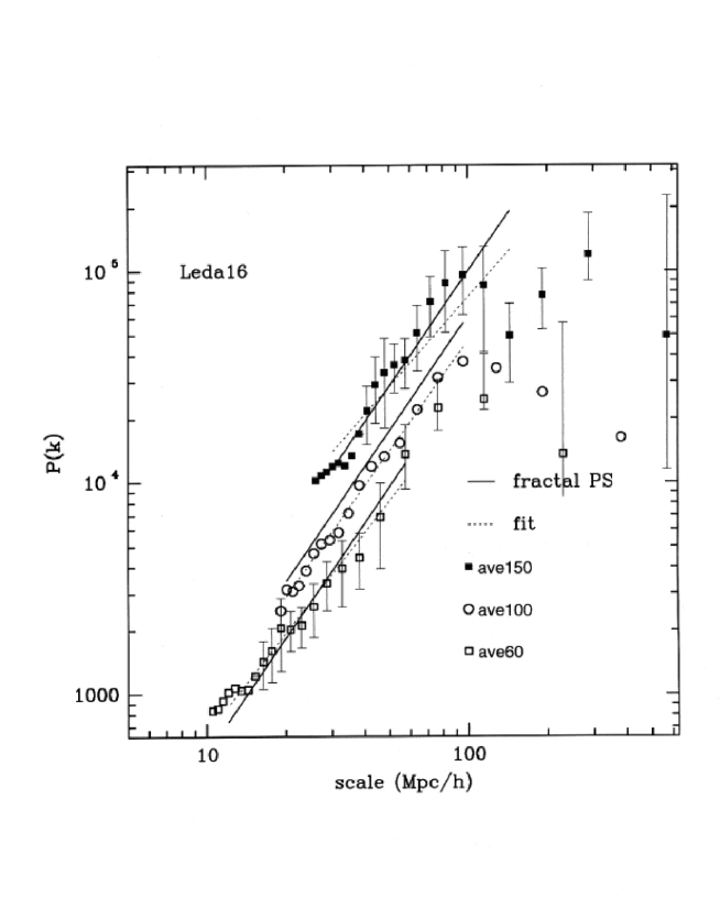
Figure 53: The four PS of the VL subsamples of LEDA-CfA at 60,78, 101 and 130 $h^{-1}Mpc$. The flattening, too, moves to higher and higher scales, as expected in the fractal view

at 60,78, 101 and 130 $h^{-1}Mpc$, respectively. (The errors, here and in what follows plots, are the scatter among fractal simulations with dimension $D=2$, with the same geometry and the same number of points as the real surveys.) As reported also in PVGH (see previous section), the spectra amplitudes scale systematically with depth. The flattening, too, moves to higher and higher scales, as expected in the fractal view (and puzzling if interpreted in terms of a constant biasing factor). In Fig.54 we compare the spectra at

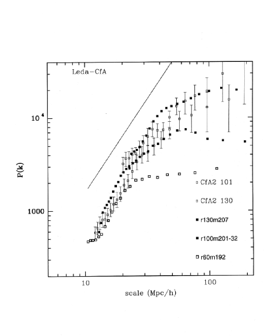
Figure 54: We compare the spectra at 101 and 130 $h^{-1}Mpc$ with the corresponding CfA spectra (PVGH). The agreement is remarkable, given that LEDA is 70% complete.

101 and 130 $h^{-1}Mpc$ with the corresponding CfA spectra (PVGH). The agreement is remarkable, given that LEDA is 70% complete at this depth.

However, this scaling effect has been often attributed to luminosity segregation (see e.g. PVGH [37]) because these volume-limited samples differ in average magnitude by increments of order $\Delta\hat{M}\approx 0.5$ . We calculated then the PS for all the fixed-depth, varying magnitude subsamples of LEDA-CfA and no evidence of luminosity biasing can be detected. For as concern LEDA-CfA, then, our conclusion is that the luminosity biasing does not explain neither the PS scale dependence, nor the constant scaling, nor the shift of the flattening scale. All three features, on the contrary, are naturally expected in a fractal clustering.

In summary we carried out a detailed investigation of the PS of galaxies in the LEDA database. The comparison with CfA2 ensures us that the incompleteness of our samples is not a source of severe distortion, at least down to about $130h^{-1}Mpc$. We found several interesting results, which complement the analysis already performed in [60]. First, we confirm the scaling of the PS with $R_{s}$, as predicted in a fractal distribution, down to 150 $h^{-1}Mpc$, with no evidence of real flattening. Second, we find that samples with widely different average luminosities have very similar spectra. The luminosity bias, where present, is neither systematic nor constant in scale. A partial exception is detected in the deepest sample LEDA16-150 (which is also the less populated, and thus more noisy, sample). Third, we find no clear evidence of a trend of $D$ versus absolute magnitude.

However, we can proceed further. The LEDA-160 PS shows in fact no sign of convergence to homogeneity. We may then take into consideration the two deepest subsamples. If the galaxy distribution is fractal to these scales, the PS should continue to scale as $R_{s}^{3-D}$. We can then scale all the spectra to $360h^{-1}Mpc$: as we show in Fig.55 for the North samples (the South ones are very similar), the fractal scaling gives again the correct amplitudes (we use here $D=1.8$), although the deepest samples are rather noisy. Notice that now this joint LEDA-360 PS spans almost five orders of magnitudes! As before, a single power law $P\sim k^{-D}$ fits all the spectrum, over two orders of magnitude in the scale, and with no sign of flattening. If one considers that we have one single parameter to model the distribution, namely the fractal dimension $D$, the alignment of all the spectra along a single line as shown in Fig.55 over such a range is indeed quite remarkable.

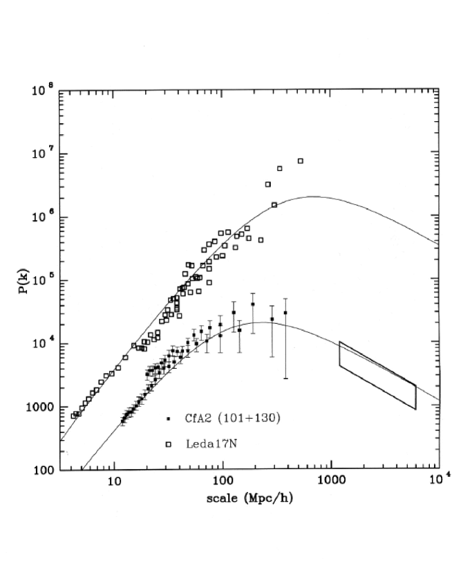
Figure 55: All the LEDA spectra to $360h^{-1}Mpc$: the fractal scaling gives again the correct amplitudes (we use here $D=1.8$), although the deepest samples are rather noisy. Notice that now this joint LEDA-360 PS spans almost five orders of magnitudes.

In the LEDA-360 PS the CDM best fit gives $\Gamma\approx.07,A\approx 10^{8.7}$, as we show in Fig.55. In terms of $\Omega$ this result is clearly rather problematic: for $h=0.5$, we get a value as low as $\Omega=0.14$. And remember that this is only an upper bound! Even more problematic the situation is looking at the bias factor, defined as the ratio of the galaxy PS $P_{g}$ to the matter PS $P_{m}$, $b^{2}(\lambda=2\pi/k)=P_{g}(k)/P_{m}(k)$. To put in agreement our LEDA-360 spectrum with the COBE data (from [111] with $n=1$, $\Omega=1$ and converted to redshift space) one would need $b(8h^{-1}Mpc)\geq 3$, $b(100h^{-1}Mpc)\geq 4.8$, and increasingly larger values at larger scales.

5 Statistical validity of galaxy catalogs

How many galaxies one needs in order to characterize correctly (statistically) the large scale distribution of visible matter ? This fundamental question is addressed in this section , and it allows us to understand some basic properties of the statistical analysis of galaxy surveys. In such a way, we are able to clarify the concept of ”fair sample”, i.e. a sample which contains a statistically meaningful information [23].

5.1 What is a fair sample ?

We have discussed in the pervious sections the properties of fractal structures and in particular we have stressed the intrinsic highly fluctuating nature of such distributions. In this perspective, it is important to clarify the concept of a ”fair sample”. Often this concept is used as synonymous of a homogeneous sample (see for example [37]) so the analysis of catalogs along the traditional lines often leads to the conclusion that we still do not have a fair sample and deeper surveys are needed to derive the correct correlation properties. A corollary of this point of view is that, since we do not have a fair sample, its statistical analysis cannot be taken too seriously.

This point of view is highly misleading because we have seen (Sec.2) that self-similar structures never become homogeneous, so any sample containing a self-similar (fractal) structure is automatically be declared ”not fair” and therefore impossible to analyze. The situation is actually much more interesting, otherwise the statistical mechanics of complex systems would not exist. Homogeneity is a property and not a condition of statistical validity of the sample. A non homogeneous system can have well defined statistical properties in terms of scale invariant correlations, that may be perfectly well defined. The whole study of fractal structures is concerned with this [15]. Therefore, one should distinguish between a ”statistical fair sample”, which is a sample in which there are enough points to derive some statistical properties unambiguously and a homogeneous sample, which is a property that can be present or not but which has nothing to do with the statistical validity of the sample itself. We have discussed in Sec.3 that even the small sample like CfA1 is statistically fair up to a distance which can be defined unambiguously (i.e $\sim 20h^{-1}Mpc$).

In the Sec.6 we define the condition to select a sample large enough to manifest the self-averaging properties of a fractal distribution. We now study a different, but related, question. Given a sample with a well defined volume, which is the minimum number of points which it should contain in order to have a statistically fair sample, even if one computes averages over all the points, such as the conditional density or the conditional average density [23] ?

5.2 Samples dilution

Consider a sample which contains a portion of a fractal structure with a lower cut-off $B$ (Sec.2). A real fractal structure in general develops between a lower and/or an upper cut-off, which respectively defines the smallest and the largest scale between which the self-similarity of the distribution can be found. (See Sec.2, and Sec.6 for a detailed discussion of the role of the lower cut-off). Given the geometry of the sample (depth $R_{s}$ and solid angle $\Omega$), we investigate what happens if we eliminate randomly more and more points from the sample. The fractal dimension and the lower cut-off are not affected by this depletion process, because they are related only to the intrinsic properties of the fractal structure. Instead, the correlation properties are more and more affected by a statistical noise as we cut the points which contribute to the statistics. This noise is superimposed to the genuine signal so that $D$ and $B$ are not changed at all, but the estimate of their values becomes noisy. Obviously, given a finite portion of the original system characterized by a lower cut-off $B$, it exists a maximum value of the number of points which we can eliminate from the structure in order to conserve the genuine statistical properties of the original distribution.

At this point we can characterize the statistical information in each VL sample more quantitatively. Suppose that the sample volume is a portion of a sphere with solid angle $\Omega$ and radius $R_{VL}$, and that the number of points inside this volume, $N_{VL}$, is

$$N_{VL}=B_{VL}\frac{\Omega}{4\pi}R_{VL}^{D}\;$$ (92)

where $B_{VL}$ takes into account the luminosity selection effect (see Sec.3 and Sec.6). The original system, inside the same volume contains

$$N=B\frac{\Omega}{4\pi}R_{VL}^{D}$$ (93)

i.e., there is not any limit in the luminosity distribution. Hence, the fraction of galaxies present in the sample can be written as

$$p=\frac{N_{VL}}{N}=\frac{B_{VL}}{B}\;.$$ (94)

In this way we can associate to each VL sample a well defined value of $p$ (see tables in the appendix). In a given sample we can randomly cut some points in the sample and define $p$ as the fraction of points which remains inside (we can clearly have a sample where both these effects are present).

The crucial point that we examine now, is whether the random or luminosity (which we assume to be random in in space) cutting of point must stop at a certain limit. Beyond this limit one does not have in the sample enough points to recover the real statistical properties of the distribution. We call statistical fair sample a sample which contains a number of points for unit volume larger than this limit. The problem is how to define this limit, or, in other words, to determine the minimal value of $p$ which allows one to recover the genuine information, for example, by the two points correlation analysis. We can proceed in two independent ways. First by analyzing the correlation properties of the VL samples of real redshift surveys and second by studying artificial distributions (see [23] for a more complete discussion of this problem).

5.3 Dilution effects on real redshift surveys

We have shown in Sec.3 that the average conditional density of some VL samples of various redshift surveys, as IRAS, APM and others, show a tendency towards a flattening. The crucial point of the IRAS data analysis, for example, is whether these samples contain enough points to allow one to detect the real statistical properties of galaxy distribution. To this aim, we compare the statistical properties of the IRAS samples with those of well-known optical ones, for example Perseus-Pisces, and we clarify the role of finite size effects in the analysis. First of all it is important to note which is the number of galaxies for unit of steradian, in the flux limited catalogs (Tab. 5). This gives a first idea of the statistical validity of the sample. To this end we note that the two IRAS catalogs, CfA1 and PP cover about the same depth but their solid angles are very different. While for CfA1 $\Omega\approx 2$ and for PP $\Omega\approx 1$, the IRAS surveys are all-sky, i.e. $\Omega\approx 4\pi$. The number of points for steradian in I-2 is about the $25\%$ of the CfA1 ones, and for I-12 it is about the $50\%$. This consideration gives a first qualitative indication that the IRAS catalogs suffer of a systematic depletion with respect to the optical ones. We can characterize this situation in a more quantitative way. We can associate to each VL sample a well defined value of $p$ (see Tab.6, and the tables in the Appendix). In the VL limited samples of the PP survey we can eliminate randomly points up to reach the fraction contained in the various IRAS samples, and then we study the behavior of the conditional density. We find that the correlation function has a clear power law behavior up to $30h^{-1}Mpc$, if the percentage remain larger than $1\div 2\%$, then it shows a crossover towards homogenization. This is clearly spurious and due to the fact that we have reached the limit of statistical validity, or fairness, of the sample.

In Tab.6 we show the characteristics of the VL samples of the PP surveys, and the corresponding VL samples of the I-12 surveys, in the same region of sky. It appears evident that the numbers for the IRAS samples are very small, and correspond to the $10\%$ of those of PP. This systematic dilution effect is the effective cause of the apparent homogenization found in IRAS samples. This explains also why IRAS galaxies are located near the brighter optical ones, and do not fill the voids. They are not more homogeneously distributed but they do not belong to a statistically fair samples. Let us examine the various redshift samples.

SURVEY	$\Omega(sr)$	Number	Galaxies/ sr
I-2 Jy	4$\pi$	2658	200
I-12 Jy	4$\pi$	5320	450
CfA1	1.8	2000	1000
PP	1	3300	3300

Table 5: Number of galaxies in various flux limited surveys

Sample	$R_{VL}$ (Mpc)	Number	Percentage
VL40IRAS	40	27	2 %
VL40PP	40	283	15 %
VL60IRAS	60	113	2.6 %
VL60PP	60	951	22
VL80IRAS	80	83	1.1 %
VL80PP	80	875	11 %

Table 6: The VL subsamples of Perseus-Pisces and of I-12 in the same sky region

5.3.1 Perseus-Pisces

In the VL samples of the Perseus-Pisces survey we eliminate randomly points up to reach the fraction contained in the various IRAS samples. We note that the correlation function has a clear power law behavior up to $30h^{-1}Mpc$ if the percentage is larger than

$$p\geq 1\div 2\%$$ (95)

then it becomes too noisy and it is not possible to recover any power law behavior (Fig.56). The quantity $p$ in Eq.95 is computed by knowing the value of $B$ in Eq.94. This is estimated from the amplitude of the conditional density and the luminosity selection factor of the sample (see Sec.3 and Sec.6 for a more detailed discussion on the determination of $B$). From various VL samples of PP, CfA1 we obtain that $B\approx 15Mpc^{-D}$.

Figure 56: The conditional density $\Gamma(r)$ for VL at 100 $h^{-1}Mpc$ (pp100) of Perseus-Pisces. The reference line (solid) has a slope of $-\gamma=-0.9$. The whole sample has 798 galaxies and we have dilute it up to 100 galaxies. In this case we are well below of the condition $p\mathrel{\hbox to0.0pt{\lower 3.0pt\hbox{$\mathchar 536\relax$}\hss}\raise 2.0pt\hbox{$\mathchar 318\relax$}}2\%$. At small scales the behavior is $1/r^{3}$ due to the sparseness of the sample. At larger distances the signal is too noisy, and does not allow one to recover the power law behavior. The sample with 200 galaxies still exhibits a power law behavior, even if the signal is more noisy.

The tendency found in Fig.56 is due to the fact that we have reached the limit of statistical validity or fairness of the sample. At small scale the conditional density exhibits a $r^{-3}$ decay that is due to the extreme dilution. The apparent homogeneous behavior shown at larger scales, in the sample with 100 galaxies, is related to the fact that in a given sample, the mean separation among galaxies $\ell$ grows when the number of points decreases ($\ell\sim(V/N)^{1/3}$; for a fractal $\ell$ is defined to be the average minimum distance between neighbour galaxies as in Sec.2), and when it becomes of the same order of the largest void present in original structure in the sample volume, the correlation properties are destroyed. This means that the artificial noise introduced by the depletion of points, have erased the intrinsic fluctuations of the original system. In this situation the system looks like an homogeneous one.

5.3.2 IRAS

In Fig.33 we show the behavior of the conditional density for various in VL of the IRAS 2 Jy survey. The deepest sample VL100, that is the sample with the lower number of galaxies, shows a $1/r^{3}$ decay at small scale, due to the extreme depletion of galaxies at these distances, followed by a almost flat behavior: this is completely spurious. We point out that the other samples VL40 and VL60 show the correct scaling behavior at the same scale at which the $\Gamma(r)$ for VL100 shows a tendency towards homogenization. The same kind of behavior can be found for the VL samples of IRAS 1.2 Jy, as shown in Fig.34. While the samples VL20 and VL60 show a clear power law behavior, the sample VL120 (North and South) exhibits a $1/r^{3}$ decay at small distances, and an almost flat behavior at larger ones (i.e. for $r\mathrel{\hbox to0.0pt{\lower 3.0pt\hbox{$\mathchar 536\relax$}\hss}\raise 2.0pt\hbox{$\mathchar 318\relax$}}10h^{-1}Mpc$).

5.3.3 SSRS1

In the case of SSRS1 we can find the same kind of behavior for the deepest VL sample (VL120 for which $p\sim 0.45\%$), as shown in Fig.57. The behavior of the conditional density has a $1/r^{3}$ decay at small scale, followed by an almost flat behavior at larger scales. Even in this case the flattening occurs where other VL samples (e.g. VL40, VL80) show a very well defined power law behavior.

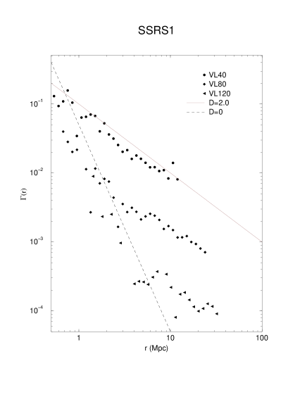
Figure 57: The conditional density $\Gamma(r)$ plotted as a function of the length scale for various volume limited of SSRS1: VL40, VL80, VL120. The difference in amplitude is simply due to the different luminosity selection in the various VL samples, and can be renormalized by taking into account the different luminosity factor of these subsamples. A reference slope of $-\gamma=-1$ is indicated by the dotted line, which corresponds to a fractal dimension of $D\approx 2$. The dashed line has a slope $-3$ (D=0).

The behavior of $\Gamma(r)$ for the sample VL120, is again, spurious and due to the extreme depletion of galaxies.

5.3.4 CfA1

The case of CfA1 is shown in Fig.58.

Figure 58: The conditional density $\Gamma(r)$ plotted as a function of the length scale for various volume limited of CfA1: VL80 and VL120. A reference slope of $-\gamma=-1.1$ is indicated by the solid line, which corresponds to a fractal dimension of $D=1.9$ up to $35\>h^{-1}Mpc$. The dashed line has a slope $-3$ (D=0).

Even in this case the deepest and more dilute sample (VL120) the conditional density shows a ”pathologic” behavior: a $1/r^{3}$ decay at small distances, followed by a flattening. The conclusion is analogous to the previous cases, i.e. this behavior is simply due to the fact that this sample is not a ”statistically fair” sample because too dilute.

5.3.5 Stromlo-APM

Finally we discuss the case of the APM-Stromlo redshift survey. Even in this case only in the deeper and more dilute samples the conditional density shows a tendency towards a flattening (see Fig.21). In Fig.59

Figure 59: The average conditional density $\Gamma^{*}(r)$ the VL12 sample of APM with progressively less galaxies (from 451 to 80 galaxies). The reference line has a slope of $-\gamma=-1$.

we show the behavior of the conditional average density for the VL12 (see appendix) in which we progressively eliminate, randomly, galaxies. While the whole sample shows very well defined fractal correlations, as the number of galaxies is reduced, the signal becomes more and more noisy. The sample with 200 galaxies shows a flattening, while the sample with 80 galaxies contains too few galaxies to allow one to reconstruct the genuine properties of the distribution.

5.3.6 Artificial fractal distributions: the role of Lacunarity

We have considered also an artificial catalog with a priori assigned properties generated with the random $\beta-$model algorithm [30]. We have found [23] that also in this case we can recover the right statistical properties only in the limit of Eq.95. Clearly Eq.95 depends on the morphological features of the realization of the fractal structure and the percentage can weakly fluctuate from a realization to another. However, even in this case in the more dilute subsample the conditional density shows a $1/r^{3}$ decay at small scale, while at larger scale it reaches an almost flat behavior. This tendency looks like the one found in the real catalogs, and it is due to the fact that we have reached the limit of statistical validity of the sample.

The role of lacunarity (Sec.2) is clearly important in the definition of a statistically fair sample. In fact, if lacunarity of the distribution is large enough (Fig.60 upper part), this means that the system is characterized by having some well defined structures and large voids (with respect to the sample size). It is clear that in this case one has to eliminate a large amount of points to destroy these structures and to lead a situation in which the remaining points seem to be homogeneously distributed. On the other hand if lacunarity is small with respect to the sample size (Fig.60 bottom part), then the typical dimension of voids is not so large and the structures are not well defined as in the previous case. In this situation, if one eliminates a certain amount of points, it is easy to destroy the fractal long-range correlations.

Figure 60: Examples of deterministic Cantor set with the same fractal dimension and different lacunarity. The lacunarity becomes larger from the bottom to the top. (Courtesy of B. Mandelbrot).

A more quantitative study is needed in order to characterize properly the role of lacunarity in this respect.

6 The decay of the radial density in wide and in deep surveys

In the previous sections we have discussed the methods that allow one to measure the conditional (average) density in real galaxy surveys. This statistical quantity is an average one, since it is determined by performing an average over all the points of the sample. We have discussed the robustness and the limits of such a measurement. We have pointed out that the estimate of the conditional density can be done up to a distance $R_{eff}$ which is of the order of the radius of the maximum sphere fully contained in the sample volume. This is because the conditional density must be computed only in spherical shells. This condition puts a great limitation to the volume studied, especially in the case of deep and narrow surveys, for which the maximum depth $R_{s}$ can be one order of magnitude, or more, than the effective depth $R_{eff}$.

In this section we discuss the measurement of the radial density in VL samples [23]. The determination of such a quantity allow us to extend the analysis of the space density well beyond the depth $R_{eff}$. The price to pay is that such a measurement is strongly affected by finite size spurious fluctuations, because it is not an average quantity. These finite size effects require a great caution [23]: the behaviour of statistical quantities (like the radial density and the counts of galaxies as a function of the apparent magnitude) that are not averaged out, present new and subtle problems.

We briefly also discuss the determination of the radial density in magnitude limited (ML) redshift surveys. In particular we show that such a measurement does not allow one to determine the fractal versus homogeneous properties of the sample. Finally we review all the determinations of the space density which we have presented in this review (i.e the conditional density and the radial density in the different VL samples of the various redshift surveys) by showing the consistency of all these measurements. This result is particularly important because it shows that all the redshift surveys discussed present consistent properties. We are able to present the behavior of the galaxy space density in the range of distances $0.5\div 1000h^{-1}Mpc$. This shows that all the available redshift samples have the same (in slope and amplitude) long-range fractal correlations with dimension $D=2\pm 0.2$, up to limits of the available samples.

6.1 Finite size effects and the behavior of the radial density

In this section we discuss the general problem of the minimal sample size which is able to provide us with a statistically meaningful information. For example, the mass-length relation for a fractal, which defines the fractal dimension, is (see Sec.2)

$$D=\lim_{r\rightarrow\infty}\frac{\log(N(<r))}{\log(r)}$$ (96)

However this relation is properly defined only in the asymptotic limit, because only in this limit the fluctuations of fractal structures are self-averaging. A fractal distribution is characterized by large fluctuations at all scales and these fluctuations determine the statistical properties of the structure. If the structure has a lower cut-off, as it is the case for any real fractal, one needs a ”very large sample” in order to recover the statistical properties of the distribution itself. Indeed, in any real physical problem we would like to recover the asymptotic properties from the knowledge of a finite portion of a fractal and the problem is that a single finite realization of a random fractal is affected by finite size fluctuations due to the lower cut-off.

In a homogeneous distribution we can define, in average, a characteristics volume associated to each particle. This is the Voronoi volume [112] $v_{v}$ whose radius $\ell_{v}$ is of the order of the mean particle separation. It is clear that the statistical properties of the system can be defined only in volumes much larger than $v_{v}$. Up to this volume in fact we observe essentially nothing. Then one begins to include a few (strongly fluctuating) points, and finally, the correct scaling behavior is recovered (Fig.61).

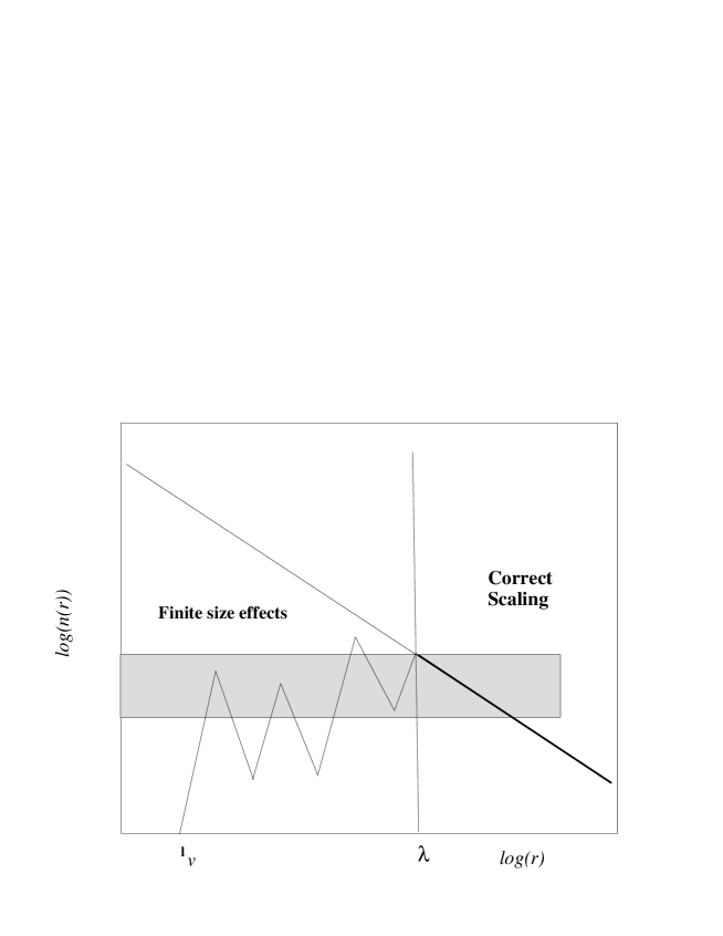
Figure 61: Behavior of the density computed from one point, in the case of a fractal distribution. At small distances below the average mean separation between neighbor galaxies, one finds no galaxies. Then the number of galaxies starts to grow, but this regime is strongly affected by finite size fluctuations. Finally the correct scaling region $r\approx\lambda$ is reached. In the intermediate region the density can be approximated roughly by a constant value. This leads to an apparent exponent $D\approx 3$. This exponent is not real but just due to the size effects.

For a Poisson sample consisting of $N$ particles inside a volume $V$ then the Voronoi volume is of the order

$$v_{v}\sim\frac{V}{N}$$ (97)

and $\ell_{v}\approx v_{v}^{1/3}$. In the case of homogeneous distributions, where the fluctuations have small amplitude with respect to the average density, one readily recovers the statistical properties of the system at small distances, say, $r\mathrel{\hbox to0.0pt{\lower 3.0pt\hbox{$\mathchar 536\relax$}\hss}\raise 2.0pt\hbox{$\mathchar 318\relax$}}5\ell_{v}$.

The case of fractal distribution is more subtle. For a self-similar distribution one has, within a certain radius $r_{0}$, $N_{0}$ objects. Following [2] we can write the mass-length relation between $N(<R)$, the number of points inside a sphere of radius $R$, and the distance $R$ of the type (see Sec.2)

$$N(<R)=BR^{D}$$ (98)

where the prefactor $B$ is related to the lower cut-offs $N_{0}$ and $r_{0}$

$$B=\frac{N_{0}}{r_{0}^{D}}\;.$$ (99)

In this case, the prefactor $B$ is defined for spherical samples. If we have a sample consisting in a portion of a sphere characterized by a solid angle $\Omega$, we write Eq.98 as

$$N(<R)=BR^{D}\frac{\Omega}{4\pi}\;.$$ (100)

In the case of a finite fractal structure, we have to take into account the statistical fluctuations. In a previous paper [23] we have proposed an argument to describe the finite size fluctuations based on extension of the concept of Voronoi length in the case of a fractal. Such an argument holds for samples in which the scaling region is of the order of the finite size effects region. Here we present a new and more general argument for the description of the finite size small scale fluctuations (see [34] for a more detailed discussion of the finite size fluctuations).

We can identify two basic kinds of fluctuations: the first ones are intrinsic $f(R)$ and are due to the highly fluctuating nature of fractal distributions while the second ones, $P(R)$, are Poissonian fluctuations. Concerning the first ones, one has to consider that the mass-length relation is a convolution of fluctuations which are present at all scales. For example one encounters, at any scale, a large scale structure and then a huge void: these fluctuations affect the power law behavior of $N(<R)$. We can quantify these effects as a modulating term around the expected average given by Eq.100. Therefore, in the observations from a single point ”i” we have

$$[N(<R)]_{i}=BR^{D}\frac{\Omega}{4\pi}\cdot f_{\Omega}(R,\delta\Omega)\;.$$ (101)

In general it is more useful to focus on the behaviour of a local quantity (as the number of points in shells) rather than an integrated one. However for the purpose of the present discussion the approximation given by Eq.101 is rather good. This equation shows that the amplitude of $N(<r)$ is related to the amplitude of the intrinsic fluctuations and not only to the lower cut-off $B$. The amplitude of the modulating term is small, compared with the expected value of $N(<R)$

$$\sqrt{|f(R)|^{2}}<BR^{D}\frac{\Omega}{4\pi}\;.$$ (102)

In general this fluctuating term depends on the direction of observation $\Omega$ and on the solid angle of the survey $\delta\Omega$ so that $f(R)=f_{\Omega}(R,\delta\Omega)$. If we have a spherical sample we get

$$\frac{1}{4\pi}\sum_{\Omega}f_{\Omega}(R,\delta\Omega)=f_{4\pi}(R)\;.$$ (103)

In general we expect that $f_{\Omega}(R,\delta\Omega)>f_{4\pi}(R)$, so that larger is the solid angle and smaller is the effect this term. If we perform the ensemble average of this fluctuating term we can smooth out its effect and we have then

$$\langle f_{4\pi}(R)\rangle_{i}=1$$ (104)

where the average $\langle....\rangle_{i}$ refers to all the occupied points in the sample. In such a way the conditional density, averaged over all the points of the sample, has a single power law behavior. We will discuss the properties of the intrinsic oscillations in a forthcoming paper [113]. Here we stress that according to Eq.101 the fluctuations in the integrated number of points in a fractal, are proportional to the number of points itself, rather than to the root mean square as in a poissonian distribution. In general [114, 115, 116, 117] it is possible to characterize these intrinsic fluctuations as log-periodic oscillations in the power law behavior. By performing an ensemble average as in Eq.104 these oscillations can be smoothed out. However for the purpose of the present paper, we limit our discussion to the approximation of Eq.101, without entering in more details.

The second $P(R)$ term is an additive one, and it takes into account spurious finite size fluctuations is simply due to shot noise. In this case we have that

$$\sqrt{|P(R)|^{2}}>BR^{D}\frac{\Omega}{4\pi}\;\;\;\mbox{if}\;\;\;R<\lambda\;$$ (105)

while $P(R)\approx 0$ for $R\mathrel{\hbox to0.0pt{\lower 3.0pt\hbox{$\mathchar 536\relax$}\hss}\raise 2.0pt\hbox{$\mathchar 318\relax$}}\lambda$. The ensemble average is, again, expected to be

$$\langle P(R)\rangle_{i}=0\;.$$ (106)

This term becomes negligible if the shot noise fluctuations are small: for example, if

$$[N(<R)]_{i}>10\sqrt{[N(<R)]_{i}}\;.$$ (107)

From this condition and Eq.101 we can have a condition on $\lambda$ (neglecting the effect of $f(R)$):

$$\langle\lambda\rangle\sim\left(10^{2}\frac{4\pi}{B\Omega}\right)^{\frac{1}{D}}$$ (108)

The minimal statistical length $\lambda$ is an explicit function of the prefactor $B$ and of the solid angle of the survey $\Omega$. This scale is a lower limit for the scaling region of the distribution: the effect of intrinsic fluctuations, described by $f(R)$, which are in general non negligible, can modulate the distance at which the scaling region is reached. This length depends also, but weakly, on the particular morphological features of the sample. Therefore it is important to stress that Eq.108 gives an order of magnitude for $\langle\lambda\rangle$, where we intend the average value over all the possible directions of observations. In different directions one can have different values for $\langle\lambda\rangle$, because of the effect of $f(r)$.

In the case of real galaxy catalogs we have to consider the luminosity selection effects. In a VL sample, characterized by an absolute magnitude limit $M_{lim}$, the mass-length relation Eq.100, can be generalized as (see Sec.3)

$$N(R,M_{lim})=BR^{D}\frac{\Omega}{4\pi}\psi(M_{lim})$$ (109)

where $\psi(M_{lim})$ is the probability that a galaxy has an absolute magnitude brighter than $M_{lim}$

$$0<\psi(M_{lim})=\frac{\int_{-\infty}^{M_{lim}}\phi(M)dM}{\Psi(\infty)}<1$$ (110)

where $\phi(M)$ is the Schecther luminosity function (normalized to unity as in Sec.3) and $\Psi(\infty)$ is the normalizing factor

$$\Psi(\infty)=\int_{-\infty}^{M_{min}}\phi(M)dM$$ (111)

where $M_{min}$ is the fainter absolute magnitude surveyed in the catalog (usually $M_{min}\approx-10\div-11$).

It is possible to compute the intrinsic prefactor $B$ from the knowledge of the conditional density $\Gamma(r)$ (see Sec.3) [2, 51]

$$\Gamma(r)=\frac{D}{4\pi}Br^{D-3}$$ (112)

computed in the VL samples and normalized for the luminosity factor (Eq.110). In the various VL subsamples of Perseus-Pisces, CfA1, and other redshift surveys (see in what follows) we find that

$$B\approx 10\div 15(h^{-1}Mpc)^{-D}$$ (113)

depending on the parameters of the Schecther function $M^{*}$ and $\delta$ (see Sec.3). From Eq.108, Eq.109 and Eq.113 we obtain for a typical volume limited sample with $M_{lim}\approx M^{*}$,

$$\langle\lambda\rangle\approx\frac{(20\div 60)h^{-1}Mpc}{\Omega^{\frac{1}{D}}}\;.$$ (114)

This is the value of the minimal statistical length that we use in what follows. In Tab. 7 we report the value of $\lambda$ for several redshift surveys. While in the case of CfA1, SSRS1, PP, LEDA and ESP we have checked that there is a reasonable agreement with this prediction, the CfA2 and SSRS2 redshift surveys are not sill published and hence in these cases we can predict the value of $\lambda$.

Survey	$\Omega(sr)$	$\lambda(h^{-1}Mpc)$
CfA1	1.8	15
CfA2 (North)	1.3	20
SSRS1	1.75	15
SSRS2	1.13	20
PP	1	40
LEDA	2 $\pi$	10
IRAS	2 $\pi$	15
ESP	0.006	300

Table 7: The minimal statistical length $\lambda$ for several redshift surveys

Given the previous discussion, we can now describe in a very simple way the behavior of $[N(<r)]_{i}$, i.e. the mass length relation measured from a generic point ”i”. Given a sample with solid angle $\Omega$, we can approximate the effect of the intrinsic and shot noise fluctuations in the following way:

$$(N(<r))_{i}=B_{1}r^{3}\;\;\;\mbox{if}\;\;r\mathrel{\hbox to0.0pt{\lower 3.0pt\hbox{$\mathchar 536\relax$}\hss}\raise 2.0pt\hbox{$\mathchar 316\relax$}}\lambda$$ (115)

i.e. the density is constant up to $\lambda$, while

$$(N(<r))_{i}=Br^{D}\;\;\;\mbox{if}\;\;r\mathrel{\hbox to0.0pt{\lower 3.0pt\hbox{$\mathchar 536\relax$}\hss}\raise 2.0pt\hbox{$\mathchar 318\relax$}}\lambda$$ (116)

so that by the condition of continuity at $\lambda$ we have

$$B_{1}=\frac{B}{\lambda^{3-D}}$$ (117)

This simple approximation is very useful in the following discussion, especially for the number counts.

6.2 Density decay from the vertex for galaxy catalogs and pencil beams

To clarify the effects of the spatial inhomogeneities and finite effects we have studied the behavior of the galaxy radial (number) density in the VL samples, i.e. the behavior of (using Eq.109 and Eq.101)

$$n_{VL}(r)=\frac{N(<r)}{V(r)}=\frac{3}{4\pi}Br^{D-3}\psi(M_{lim})\cdot f_{\Omega}(r,\delta\Omega)$$ (118)

One expects that, if the distribution is homogeneous the density is constant, while if it is fractal it decays as power law.

When one computes the conditional average density (see Sec.3), one indeed performs an average over all the points of the survey. In particular, as we have already discussed, we limit our analysis to a size defined by the radius of the maximum sphere fully contained in the sample volume, and we do not make use any treatment of the sample boundaries. On the contrary Eq.118 is computed only from a single point, the origin. This allows us to extend the study of the spatial distribution up to very deep scales. The price to pay is that this method is strongly affected by statistical fluctuations and finite size effects.

The effect of the finite size spurious fluctuations for a fractal distribution is shown Fig.61: at small distances one finds almost no galaxies because we are below the average mean separation between neighbor galaxies $\ell$. Then the number of galaxies starts to grow, but this regime is strongly affected by finite size fluctuations. Finally the correct scaling region $r\approx\lambda$ is reached. This means, for example, that if one has a fractal distribution, there is first a raise of the density, due to finite size effects and characterized by strong fluctuations, because no galaxies are present before a certain characteristic scale. Once one enters in the correct scaling regime for a fractal the density starts to decay as a power law. So in this regime of raise and fall with strong fluctuations there is a region in which the density can be approximated roughly by a constant value. This leads to an apparent exponent $D\approx 3$, so that the integrated number grows as $N(<r)\sim r^{3}$. This exponent is therefore not a real one but just due to finite size fluctuations. Of course, depending on the survey orientation in the sky, one can get an exponent larger or smaller than $3$, but in general this is the more frequent situation (see below). Only when a well defined statistical scaling regime has been reached, i.e. for $r>\lambda$, one can find the genuine scaling properties of the structure, otherwise the behavior is completely dominated by spurious finite size effects (for seek of clarity in this discussion we do not consider the effect of $f(r)$ in Eq.101)

The question of the difference between the integration from the origin (radial density) and correlation properties averaged over all points lead us to a subtle problem of asymmetric fluctuations in a fractal structure. From our discussion, exemplified by Fig.61, the region between $\ell$ and $\lambda$ corresponds to an underdensity with respect to the real one. However we have also showed that for the full correlation averaged over all the points, as measured by $\Gamma(r)$, the correct scaling is recovered at distances appreciably smaller than $\lambda$. This means that in some points one should observe an overdensity between $\ell$ and $\lambda$. However, given the intrinsic asymmetry between filled and empty regions in a fractal, only very few points show the overdensity (a fractal structure is asymptotically dominated by voids). These few points nevertheless have, indeed, an important effect on the average values of the correlations. This means that, in practice, a typical points shows an underdensity up to $\lambda$ as shown in Fig.61. The full averages instead converge at much shorter distances. This discussion shows the peculiar and asymmetric nature of finite size fluctuations in fractals as compared to the symmetric Poissonian case. For homogeneous distribution [23] the situation is in fact quite different. Below the Voronoi length $\ell_{v}$ there are finite size fluctuations, but for distances $r\mathrel{\hbox to0.0pt{\lower 3.0pt\hbox{$\mathchar 536\relax$}\hss}\raise 2.0pt\hbox{$\mathchar 318\relax$}}(2\div 4)\ell_{v}$ the correct scaling regime is readily found for the density. In this case the finite size effects do not affect too much the properties of the system because a Poisson distribution is characterized by small amplitude fluctuations.

6.2.1 Perseus-Pisces

We have computed the $n(r)$ in the various VL samples of Perseus-Pisces redshift survey, and we show the results in Fig.62. In the less deeper VL samples (VL70, VL90) the density does not show any smooth behavior because in this case the finite size effects dominate the behavior as the distances involved are $r<\lambda$ (Eq.114). At about the same scales we find a very well defined power law behavior by the correlation function analysis (see Sec.3). In the deeper VL samples (VL110, VL130) a smooth behavior is reached for distances larger than the scaling distance ($\Omega=0.9\,sr$) $r\approx\lambda\sim 50h^{-1}Mpc$. The fractal dimension is $D\approx 2$ as one measures by the correlation function.

Figure 62: The spatial density $n(r)$ computed in the VL sample cut at $70,90,110,130h^{-1}Mpc$ . In the case of VL70 and VL90 the density is dominated by large fluctuations and it has not reached the scaling regime. In the samples VL110 and VL130 the density is dominated by large fluctuations only at small distances, while at larger distances, after the Perseus Pisces chain at $50h^{-1}Mpc$, a very well defined power law behavior is shown, with the same exponent of the correlation function (i.e. $D=2$)

For relatively small volumes it is possible to recover the correct scaling behavior for scales of order of $\ell$ (instead of $\sim 10\ell$) by averaging over several samples or, as it happens in real cases, over several points of the same sample when this is possible. Indeed, when we compute the correlation function we perform an average over all the points of the system even if the VL sample is not deep enough to satisfy the condition expressed by Eq.114. In this case the lower cut-off introduces a limit in the sample statistics (Sec.5).

6.2.2 CfA1

In the case of CfA1 ($\Omega=1.8$) we obtain that $\lambda\approx 15h^{-1}Mpc$. We compute the behavior of the radial density and we show the results in Fig.63:

Figure 63: The spatial density $n(r)$ computed in various VL sample of CfA1 (cut in absolute magnitude). A very well defined power law behavior with $D\approx 1.9$ is shown for $r\mathrel{\hbox to0.0pt{\lower 3.0pt\hbox{$\mathchar 536\relax$}\hss}\raise 2.0pt\hbox{$\mathchar 318\relax$}}15h^{-1}Mpc\approx\lambda$.

in the various cases the agreement with Eq.114 is quite good. The sample VL20 (cut at the absolute magnitude $M=-20$) shows a raising of the radial density at $\sim 70h^{-1}Mpc$. This is a typical fluctuation due to the presence of structures, which characterizes at fractal distribution at any scale, and which is not smoothed out because $n(r)$ is not averaged over all the galaxies. These intrinsic fluctuations are described by the modulating function $f(r)$ in Eq.101.

6.2.3 SSRS1

In the case of SSRS1 the solid angle is $\Omega=1.75\;sr$, and, as for CfA1, we obtain that $\lambda\sim 15h^{-1}Mpc$. We show in Fig.64

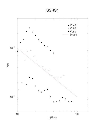
Figure 64: The spatial density $n(r)$ computed in some VL samples of SSRS1. A very well defined power law behavior with $D\approx 2$ is shown for $r\mathrel{\hbox to0.0pt{\lower 3.0pt\hbox{$\mathchar 536\relax$}\hss}\raise 2.0pt\hbox{$\mathchar 318\relax$}}15h^{-1}Mpc\approx\lambda$.

the behavior of $n(r)$ is the VL samples of this catalog. Even in this case the decay of the radial density shows a $1/r$ behaviour (i.e. $D\approx 2$), in agreement with the results obtained by the conditional density. The sample VL80 is more noisy due to the large depletion of points (see Sec.5).

6.2.4 LEDA

LEDA is an all-sky survey, a part the region corresponding to the galactic plane. The scaling region begins at $\sim 10h^{-1}Mpc$ and it extends up to the limit of the sample, as shown in Fig.65.

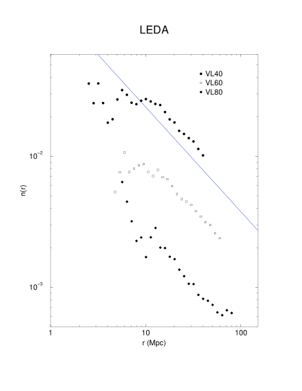
Figure 65: The spatial density $n(r)$ computed in some VL samples of LEDA145. A very well defined power law behavior with $D\approx 2$ is shown for $r\mathrel{\hbox to0.0pt{\lower 3.0pt\hbox{$\mathchar 536\relax$}\hss}\raise 2.0pt\hbox{$\mathchar 318\relax$}}10h^{-1}Mpc\approx\lambda$.

The scaling behavior is reached for distances larger $r\mathrel{\hbox to0.0pt{\lower 3.0pt\hbox{$\mathchar 536\relax$}\hss}\raise 2.0pt\hbox{$\mathchar 318\relax$}}15h^{-1}Mpc$, and the fractal dimension is $D\approx 2$ even in this case. The sample VL80 shows a fluctuation near the boundary, and has a $1/r^{3}$ decay up to $\sim 10h^{-1}Mpc$ due to the depletion of points in this sample.

6.2.5 Las Campanas Redshift Survey

In the case of LCRS it is not possible to compute the radial density. This is because the survey is limited by a double cut in apparent magnitude, a lower and an upper one (see Sec.3). Hence it is possible to have VL samples in a certain range of distances, the lower limit not being the origin. Therefore, in this case it is possible to study the derivative of $n(r)$

$$\frac{dn(r)}{dr}\sim r^{-\gamma-1}\;.$$ (119)

Clearly this is not an integrated quantity, as $n(r)$, and hence it is much noisy than the radial density. We show in Fig.66 the results of such determinations.

Figure 66: The spatial density $dn(r)/dr\cdot r$ computed in some VL samples of LCRS. The solid line has a slope $-\gamma=-1$.

Unfortunately it is not possible to obtain a VL sample that covers a large extension in depth. In this case it is not possible to detect any specific value for $\lambda$. There are large fluctuations in the space distribution (Fig.66) and the samples SL12-2565 and SL12-36 show a power law behavior in the range $\sim 200\div 600h^{-1}Mpc$ with $D\approx 2$. This behavior is not so very well defined because $dn/dr$ is neither an integrated quantity (as $n(r)$), nor it is averaged as $\Gamma(r)$, and the extension in depth is small in log scale. The samples SL12-125 and SL12-153 show a highly fluctuating behavior for $dn/dr$. This is due to the fact that the scaling is not reached at all in these samples. We stress that an homogeneous distribution at these scales should exhibits a flat behavior without large fluctuations.

6.2.6 Stromlo-APM Redshift Survey

The same problem of LCRS is present also in the case of Stromlo-APM Redshift Survey, for what concerns the construction of the VL samples. Even in this case we have to estimate the derivative of radial density, rather than the radial density itself. The behavior of $dn(r)/dr\cdot r$ for various VL samples of SARS is shown in Fig.67.

Figure 67: The spatial density $dn(r)/dr\cdot r$ computed in a VL samples of APM. The solid line has a slope $-\gamma=-1$.

In this case there are the same problems discussed for the case of LCRS: a very fluctuating behavior and a small range of distance where it is possible to study the power law decay of the radial density. These results are again compatible with a fractal distribution and not with an homogeneous one.

6.2.7 ESP

As the redshifts involved are quite large a particular care is devoted to the construction of the VL subsamples for the case of ESP. We have used various distance-redshift ($d(z)$) and magnitude-redshift ($m(z)$) relations [9].

1) Friedmann-Robertson-Walker relations

If we assume a particular cosmological model as the FRW, we use the following comoving distance-redshift relation

$$d(z,q_{0})=\frac{c}{H_{0}}\frac{zq_{0}+(q_{0}-1)(\sqrt{2q_{0}z+1}-1)}{q_{0}^{2}(z+1)}\;\;h^{-1}Mpc$$ (120)

and we have used the following values of the deceleration parameter $q_{0}=0.03,0.5$ and $1$. The data are selected in the blue-green and even if the redshift of galaxies are moderate ($z\leq 0.2$) K-corrections are needed to compute the absolute magnitude of galaxies [44]. The corresponding magnitude-redshift relation is

$$m-M=25+5\log_{10}\left(d(z,q_{0})(1+z)\right)+a(T)z$$ (121)

where we have used the functional forms of the K-correction $a(T)z$ as a function of redshift from [118]. $a(T)$ depends on the morphological type $T$ and goes from $a\sim 2$ for the Scd galaxies to $a\sim 3.7$ for the E/S0 galaxies. It is not possible to apply the K-correction to each morphological type because over the $\>17^{th}$ magnitude it is not possible to recognize the Hubble type from visual inspection. To overcame this problem (following [44]) we have adopted a statistical approach: we have assumed various percentage of late and early-type galaxies. The observed percentage in nearer samples is $\>70\%$ of late and $\>30\%$ of early type of galaxy. We have performed a number of tests by varying these percentages to show that the final result depends weakly on the adopted values. We note that varying these percentages change the number of points in the VL subsamples as the absolute magnitude can change of about $1$ in absolute value.

The behavior of the number-distance relation in the standard FRW model depends strongly on the value of the deceleration parameter $\>q_{0}$ for high redshift $\>z>0.5$, while for $\>z<0.2$ the relativistic corrections are very small for all reasonable $\>q_{0}$.

All the sample show a highly fluctuating behavior for the space density (Fig.68).

Figure 68: The spatial density $n(r)$ computed in a VL samples of ESP, using $q_{0}=0.5$. The power law behavior with $D\approx 2$ is defined for $r\mathrel{\hbox to0.0pt{\lower 3.0pt\hbox{$\mathchar 536\relax$}\hss}\raise 2.0pt\hbox{$\mathchar 318\relax$}}300h^{-1}Mpc$ in all the samples.

At $\lambda\sim 300h^{-1}Mpc$ the scaling region is reached. Again, as in the previous case, we stress that an homogeneous distribution (say at $50h^{-1}Mpc$) would show a very smooth and flat behavior for $n(r)$ at these distance scales. This is clearly not the case.

2.) The Euclidean relations

It is very, interesting, in our opinion to study also the case of a purely Euclidean space. In this case we can write the $d(z)$ relation simply as:

$$d=\frac{c}{H_{0}}z$$ (122)

and the $m(z)$ relation (without K-corrections):

$$m-M=5\log_{10}\left(d(z)\right)+25\;.$$ (123)

In this case the volume grows as $\sim z^{3}\sim d^{3}$. The behavior of the radial density in the Euclidean case is reported in Fig.69.

Figure 69: The spatial density $n(r)$ computed in a VL samples of ESP. A the power law behavior with $D\approx 2$ is shown for $r\mathrel{\hbox to0.0pt{\lower 3.0pt\hbox{$\mathchar 536\relax$}\hss}\raise 2.0pt\hbox{$\mathchar 318\relax$}}300h^{-1}Mpc\approx\lambda$, even though with strong fluctuations

From this figure it is possible to see the effect of the finite size fluctuations: the scaling region begins at $\lambda\sim 300\div 320h^{-1}Mpc$ for all the VL subsamples. For smaller distances the statistical fluctuations dominate the behavior of $n(r)$. The different normalization in the various VL subsamples is due to the different absolute magnitude limit $M_{lim}$ which defines each VL subsample. To normalize the behavior of $n(r)$ we divide it for a luminosity factor (see Sec.6.5). It seems that in this case the power law behavior for $r\mathrel{\hbox to0.0pt{\lower 3.0pt\hbox{$\mathchar 536\relax$}\hss}\raise 2.0pt\hbox{$\mathchar 318\relax$}}\lambda\approx 320h^{-1}Mpc$ is better defined than in the previous case. The fractal dimension turns out to be $D\approx 2.2$.

The K-correction can change the absolute magnitude of a unit. This correction is a systematic effect for each morphological type. As we put these correction in a random manner we are mixing a systematic effect with a random correction. In this way we can onlycheck the stability of the results but we cannot hope to obtain a better fit (see Fig.70). Hence we conclude that the fractal dimension is $\>D\approx 2$ is a substantially stable result.

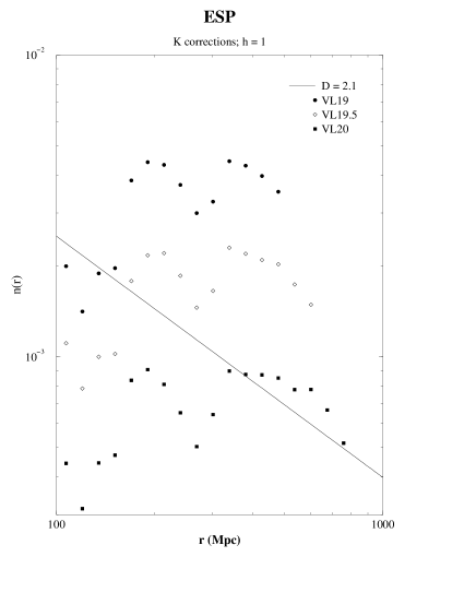
Figure 70: The spatial density $n(r)$ computed in a VL samples of ESP applying the random K-corrections as explained in the text. A very well defined power law behavior with $D\approx 2$ is shown for $r\mathrel{\hbox to0.0pt{\lower 3.0pt\hbox{$\mathchar 536\relax$}\hss}\raise 2.0pt\hbox{$\mathchar 318\relax$}}320h^{-1}Mpc\approx\lambda$.

6.2.8 IRAS

As for the case of LEDA, also IRAS is an all sky survey. However the IRAS samples are limited by the weak statistics which characterizes these surveys, as discussed in Sec.3 and Sec.5. We show in Fig.71

Figure 71: The spatial density $n(r)$ computed in a VL samples of IRAS 1.2 Jy. The power law behavior with $D\approx 2$ is shown for distances $\mathrel{\hbox to0.0pt{\lower 3.0pt\hbox{$\mathchar 536\relax$}\hss}\raise 2.0pt\hbox{$\mathchar 318\relax$}}10h^{-1}Mpc$.

the results of the determination of the radial density in various VL samples of the survey IRAS $1.2Jy$ (North). A power law behavior is defined for $r\mathrel{\hbox to0.0pt{\lower 3.0pt\hbox{$\mathchar 536\relax$}\hss}\raise 2.0pt\hbox{$\mathchar 318\relax$}}10h^{-1}Mpc$, as in the case of LEDA, with $D\approx 2$, up to $\sim 60h^{-1}Mpc$. The deepest VL sample (VL80) shows an $1/r^{3}$ decay at small scale and a flat behavior at larger scales. This is again interpreted as due to the extreme dilution of galaxies in this sample (see Sec.5).

6.3 Radial density in magnitude limited surveys

It is usually measured in literature the number of galaxies $N_{ml}(r)$ as a function of distance in a magnitude limited surveys. Some authors (e.g. Davis [19]) claims that from the behavior of $N_{ml}(r)$ it is possible to distinguish between a fractal and an homogeneous distribution. Contrary to this result, we show that such a measurement depends only on the luminosity selection function of the survey, and very weakly from the value of the fractal dimension.

Assuming, as in Sec.3, the independence of the space density on the luminosity one, we can compute the number of galaxies in the bin of distances $\Delta R$ in a magnitude limited survey ($m_{lim}$ is the apparent magnitude limit) as

$$N_{ml}(R)=\int_{R}^{R+\Delta R}\rho(r)d^{3}r\int_{-\infty}^{M(r)}\phi(M)dM$$ (124)

(we neglect relativistic corrections), where

$$M(r)=m_{lim}-5\log(r)-25$$ (125)

From Eq.124 it follows that $N_{ml}(r)$is a function of four parameters: the fractal dimension $D$ and the prefactor $B$ and the two parameters of the luminosity function $\delta$ and $M^{*}$. In Fig.72 we show the behavior of $N_{ml}(r)$ with different values of the three parameters, in a survey with fixed $m_{lim}$. The major effect is due to the luminosity selection function rather than to the space distribution. This is the reason why one has to use VL samples rather than ML ones, in order to study the behavior of the space density.

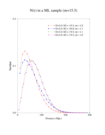
Figure 72: The spatial density $N_{ml}(r)$ (per bin of $10h^{-1}Mpc$) in a magnitude limited survey ($m_{lim}=15.5$) for various values of the parameters $D$, $\delta$ and $M^{*}$. It is clear that the behavior of $N_{ml}(r)$ is mostly due on the luminosity selection function of the survey, and hence $\delta$ and $M^{*}$, rather than on the fractal dimension $D$. This is the reason why one has to use VL samples in order to study the behavior of the space density.

All the determinations of the space density (or of the amplitude of luminosity function) in magnitude limited samples are seriously affected by this bias (see for example [45]).

6.4 Pencil beams and very deep surveys

Deep ”pencil beams” surveys cover in general very narrow angular size ($\sim 1^{\circ}$) and extend to very deep depths ($z\mathrel{\hbox to0.0pt{\lower 3.0pt\hbox{$\mathchar 536\relax$}\hss}\raise 2.0pt\hbox{$\mathchar 318\relax$}}0.2$). These narrow shots through deep space provide a confirmation of strong inhomogeneities in the galaxy distribution.

One of the most discussed results obtained from pencil-beams surveys has been the claimed detection of a typical scale in the distribution of galaxy structures, corresponding to a characteristic separation of $128h^{-1}Mpc$ [43]. However in the last five years several other surveys, in different regions of the sky, do not find any evidence for such a periodicity. In particular, Bellanger & De Lapparent [119], by analyzing a sample of 353 galaxies in the redshift interval $0.1\mathrel{\hbox to0.0pt{\lower 3.0pt\hbox{$\mathchar 536\relax$}\hss}\raise 2.0pt\hbox{$\mathchar 316\relax$}}z\mathrel{\hbox to0.0pt{\lower 3.0pt\hbox{$\mathchar 536\relax$}\hss}\raise 2.0pt\hbox{$\mathchar 316\relax$}}0.5$, concluded that these new data contain no evidence for a periodic signal on a scale of $128h^{-1}Mpc$. Moreover they argue that the low sampling rate of [43] is insufficient for mapping the detailed large-scale structure and it is the real origin of the apparent periodicity.

On the other hand, Willmer et al.[120] detect four of the five nearest peaks of the galaxies detected by [43], because their survey is contiguous to that of [43], in the sky region near the north Galactic pole. Moreover Ettori et al.[121] in a survey oriented in three small regions around the South Galactic Pole do not find any statistically periodic signal distinguishable from noise. Finally Cohen et al.[122] by analyzing a sample of 140 objects up to $z\sim 0.8$, find that there is no evidence for periodicity in the peak redshifts.

In a pencil-beam survey one can study the behavior of the linear density along a tiny but very long cylinder. The observed galaxy distribution corresponds therefore to the intersection of the full three dimensional galaxy distribution with one dimensional cylinder [2]. In this case, from the law of codimension additivity [14, 2] (see Sec.2), one obtains that the fractal dimension of the intersection is given by

$$D_{I}=D+d_{pc}-d\approx D+1-3\approx 0$$ (126)

where $D$ is the galaxy distribution fractal dimension, embedded in a $d=3$ Euclidean space, and $d_{pc}=1$ is the dimension of the pencil beam survey. This means that the set of points visible in a randomly oriented cylinder has dimension $D_{I}\approx 0$. In such a situation the power law behavior is no longer present and the data should show a chaotic, featureless nature strongly dependent on the beam orientation. If the galaxy distribution becomes instead homogeneous above some length, shorter than the pencil beam depth, one has the regular situation $D_{I}=1$ and a well defined density must be observed.

We stress that in any of the available pencil beams surveys, one can detect tendency towards an homogeneous distribution. Rather, all these surveys show a very fluctuating signal, characterized by the presence of galaxy structures. Some authors [41] claim to detect the end greatness (i.e. that the galaxy structures in the deep pencil beams are not so different from those seen in nearby sample - as the Great Wall), or that [119] the dimension of voids does not scale with sample size, by the visual inspection of these surveys. However one should consider in these morphological analyses, that one is just looking at a convolution of the survey geometry, which in general are characterized by very narrow solid angles, and large scale structures, and that in such a situation, a part from very favorable cases, one may detect portions of galaxy structures (or voids).

Finally we note that if the periodicity would be present, the amplitude of the different peaks is very different from each other, and an eventual transition to homogeneity in a periodic lattice, should be, for example, ten times the lattice parameter, i.e. $\mathrel{\hbox to0.0pt{\lower 3.0pt\hbox{$\mathchar 536\relax$}\hss}\raise 2.0pt\hbox{$\mathchar 318\relax$}}1000h^{-1}Mpc$ !

6.5 Consistency of the various catalogs and summary of the galaxy correlation properties: fractal behavior from $0.5h^{-1}Mpc$ to $1000h^{-1}Mpc$

In this section and in Sec.3 we have discussed two different determinations of the galaxy space density, i.e the radial density and the conditional density respectively. Now we show the consistency of these measurements in each of the presented galaxy samples, and then we show the consistency of the correlation properties in the various galaxy catalogs. In particular, the new analysis shows that all the available data are consistent with each other and show fractal correlations with dimension $D=2.0\pm 0.2$ up to the deepest scale probed up to now by the available redshift surveys, i.e. $\sim 1000h^{-1}Mpc$. The distribution of luminous matter in the Universe is therefore fractal and not homogeneous. The evidence for this is very strong up to $\sim 150h^{-1}Mpc$, due to the statistical robustness of the data, and progressively weaker (statistically) at larger distances due to the limited data available.

6.5.1 Normalization of the density in different VL samples

In Sec.3 we have already defined the luminosity factor which is associated to each VL sample. Both the conditional density and the radial density measure the space density of galaxies. As long as the space and the luminosity density can be considered independent, the normalization of $\Gamma(r)$ and $n(r)$ in different VL samples can be simply done by dividing their amplitudes for the corresponding luminosity factors. Of course such a normalization is parametric, because it depends on the two parameters of the luminosity function $\delta$ and $M^{*}$ (see Sec.3 and Sec.8). For a reasonable choice of these two parameters we find that the amplitude of the conditional and radial density matches quite well in different VL samples. In particular:

• (1) For CfA1, PP, ESP, LEDA and APM the parameters of the luminosity function are $\delta=-1.1$ and $M^{*}=-19.5$. All these surveys have been selected in the B-band, and hence the luminosity function is the same.

• (2) For SSRS1 the selection criteria have been chosen in the apparent diameter $d$, and hence we use the linear-diameter function, rather than the luminosity function for the normalization of the amplitude in different VL samples. We use the diameter function:

  $$N(D)dD=N_{0}\cdot exp(-\delta_{d}\cdot D)dD$$ (127)

  where $D$ is the absolute diameter (in Kpc), $\delta_{d}=0.109$ and $N_{0}$ is a constant [64]. The shape of this linear-diameter function is similar to the Schecther one for magnitudes.

• (3) Galaxies in LCRS have been measured in the $r$ band, so that we have used the luminosity function given by [41]. i.e. a Schecther like function with parameters $\delta=-0.9$ and $M^{*}=-20.03$.

• (4) The two IRAS surveys have been measured in the near infrared. In this case we have normalized the amplitude of the density using the $IR$ luminosity function [123].

We find that in all the cases (1)-(4) the density amplitude in the different VL samples match quite well (see Figs.73-74).

Figure 73: The spatial conditional average density $\Gamma^{*}(r)$ computed in some VL samples of Perseus-Pisces, CfA1, ESP and LEDA and normalized to the corresponding luminosity factor.

Figure 74: The spatial conditional average density $\Gamma^{*}(r)$ computed in some VL samples of APM, LCRS, SSRS1, IRAS $1.2Jy$ and normalized to the luminosity factor.

6.5.2 Normalization of the average conditional density to the radial density

Figure 75: The conditional average density $\Gamma^{*}(r)$ (filled points) and the radial density $n(r)$ (open points) computed in a VL sample of Perseus-Pisces.

Figure 76: The conditional average density $\Gamma^{*}(r)$ (filled points) and the radial density $n(r)$ (open points) computed in a VL sample of CfA1.

The normalization of the conditional density to the radial density should take into account only a trivial $(3/D)$ factor. However for example in the case of PP and CfA1 there is a certain different (about a factor $2\div 5$) between the amplitude of the conditional density and of the radial one, even if one has properly normalized the amplitude of these functions, as shown in Fig.75 and Fig.76. As we have already mentioned in (see Eq.101), this difference can be understood considering the fact that $N(<R)$ is modulated by a function $f(R)$ which takes into account the presence of not smoothed out fluctuations at all scales. Usually, galaxy surveys are pointed towards some great large scale structures. If one computes the conditional density in spherical shells, one is properly making the average, taking into account the structures and the voids present in the sample. If, on the other hand, one measures the radial density from one point only, one is biased by the fact that the survey, by construction, does not contain voids and structures of the same size. The dimension of the structures is limited by the boundaries of the sample. Hence, if the survey contains a large scale structure cannot contain also a corresponding large scale void. This asymmetry is the real effect which shifts the amplitude of the radial density of a small factor beyond that of the conditional density. However we stress that only the conditional density measures the correct amplitude, while the radial density is biased by the modulating effect of $f(R)$, and hence by the geometry of the survey.

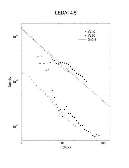
Figure 77: The conditional density $\Gamma(r)$ and the radial density $n(r)$ computed in a VL sample of LEDA14.5. The amplitude in this case match quite well because LEDA is an all-sky survey.

Figure 78: The conditional average density $\Gamma^{*}(r)$ and the radial density $n(r)$ computed in a VL sample of IRAS 1.2 Jy. The amplitude in this case match quite well because IRAS is an all-sky survey.

If the surveys are all-sky ones, then the amplitudes of the conditional and the radial density should match better, because in this case by measuring $n(r)$ one properly averages voids and structures. In other terms, as we have previously discussed, this means that $f_{\Omega}(R,\delta\Omega)>f_{4\pi}$. This can be seen, for example, in the case of LEDA (Fig.77), or IRAS (Fig.78).

6.5.3 Normalization of the density in different surveys

Figure 79: The spatial density $\Gamma(r)$ computed in some VL samples of CfA1 and Perseus-Pisces cut at the same absolute magnitude. The solid line corresponds to a fractal dimension $D=2$

The normalization of $\Gamma(r)$ (or $n(r)$) in the surveys CfA1 and Perseus-Pisces can be done without any additional factor. If one compares VL with the same cut in absolute magnitude no normalization is needed (see Fig.79).

For the case of Stromlo-APM Redshift Survey one has to take into account the random sampling, and hence one has to multiply the amplitude of the density for $20$ (see Sec.3). The same factor must be taken into account in the case of LEDA, even if the factor varies according to the sample considered (see Sec.3 for a detailed discussion of the LEDA criteria).

The case of ESP is more complex: because of the presence of the ”holes” in the survey one obtains a lower value of amplitude of the correlation function (see Sec.3). For this reason the comparison is not possible as in the previous cases. As we are dealing with a fractal distribution, we cannot estimate the missing points through a simple factor, as one may do in the case of an homogeneous distribution.

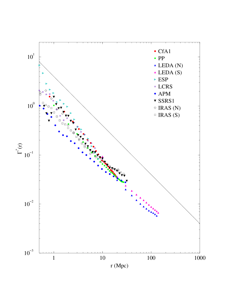
Figure 80: The spatial density $\Gamma(r)$ computed in some VL samples of CfA1, PP, LEDA, APM, ESP, LCRS, SSRS1, IRAS and ESP and normalized to the corresponding factor, as explained in the text.

In the case of SSRS1, LCRS and IRAS the normalization can be done considering the different luminosity selection criteria adopted in each case. For the case of LCRS one has to take into account also the random sampling adopted in this case. We show in Fig.80 the normalization of all the surveys. In Fig.81

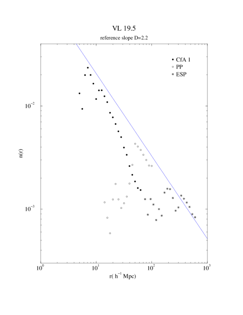
Figure 81: The spatial density $n(r)$ computed in some VL samples with the same cut in absolute magnitude of CfA1, PP and ESP.

we show the determinations of the radial density in VL with the same cut in absolute magnitude, in different surveys: PP, CfA1, and ESP. In these cases the match of the amplitudes and exponents is quite good.

Figure 82: Full correlation analysis for the various available redshift surveys in the range of distance $0.5\div 1000h^{-1}Mpc$. A reference line with slope $-1$ is also shown, which corresponds to fractal dimension $D=2$.

Figure 83: Traditional analyses based on the function $\xi(r)$ of the same galaxy catalogs of the previous figure. The usual analysis is based on the a priori untested assumptions of analyticity and homogeneity. These properties are not present in the real galaxy distribution and the results appear therefore rather confusing. This lead to the impression that galaxy catalogs are not good enough and to a variety of theoretical problems like the galaxy-cluster mismatch, luminosity segregation, linear and non-linear evolution, etc. This situation changes completely and becomes quite clear if one adopts the more general conceptual framework that is at the basis the previous figure

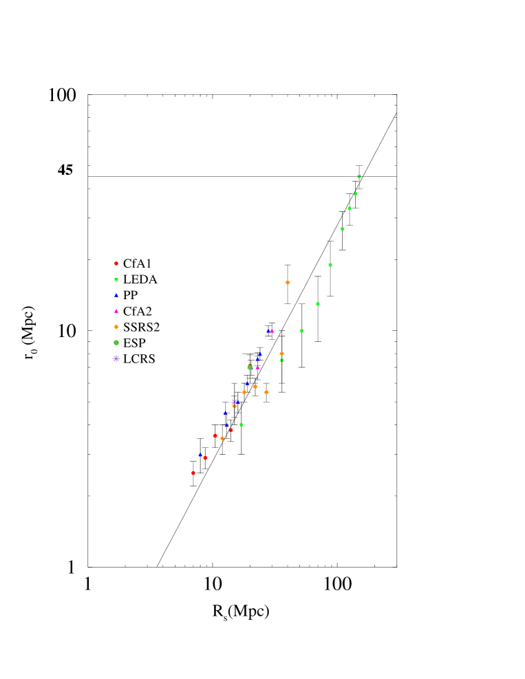
Figure 84: Determinations of the so called ”correlation-length” $r_{0}$ in the available redshift surveys. The agreement among the different surveys is quite good. A linear dependence of $r_{0}$ on the sample size $R_{eff}$ is shown. The observed is in agreement with the fractal prediction.

Finally in Fig.82 we show the final diagram with all the available surveys. It is remarkable to stress that the amplitudes and the slopes of the different surveys match quite well. From this figure we conclude that galaxy correlations show very well defined fractal properties in the entire range $0.5\div 1000h^{-1}Mpc$ with dimension $D=2\pm 0.2$. Moreover all the surveys are in agreement with each other.

It is interesting to compare the analysis of Fig.82 with the usual one, made by the function $\xi(r)$, for the same galaxy catalogs. This is reported in Fig.83.

From this point of view, the various data the various data appear to be in strong disagreement with each other. This is due to the fact that the usual analysis looks at the data from the prospective of analyticity and large scale homogeneity (within each sample). These properties have never been tested and they are not present in the real galaxy distribution so the result is rather confusing (Fig.83). Once the same data are analyzed with a broader perspective the situation becomes clear (Fig.82) and the data of different catalogs result in agreement with each other. It is important to remark that analyses like those of Fig.83 have had a profound influence in the field in various ways: first the different catalogs appear in conflict with each other. This has generated the concept of not fair samples and a strong mutual criticism about the validity of the data between different authors. In the other cases the discrepancy observed in Fig.83 have been considered real physical problems for which various technical approaches have been proposed. These problems are, for example, the galaxy-cluster mismatch, luminosity segregation, the richness-clustering relation and the linear non-linear evolution of the perturbations corresponding to the ”small” or ”large” amplitudes of fluctuations. All this problematic situation is not real and it arises only from a statistical analysis based on inappropriate and too restrictive assumptions that do not find any correspondence in the physical reality. It is also important to note that, even if the galaxy distribution would eventually became homogeneous at larger scales, the use of the above statistical concepts is anyhow inappropriate for the range of scales in which the system shows fractal correlations as those shown in Fig.82.

In Fig.84 we report the various determinations of the so called ”correlation; length” $r_{0}$ as a function of the sample size in the available redshift surveys. Also in this case $r_{0}$ is just a linear fraction of the sample depth, as expected in the fractal case. It is worth to notice that all the available catalogs give a consistent results for such a measurement.

7 Number counts and angular correlations

The most complete information about galaxy distribution comes from the full three dimensional samples, while the angular catalogs have a poorer qualitative information, even if usually they contain a much larger number of galaxies. However, one of the most important tasks in observational astrophysics, is the determination of the $\log N-\log S$ relation for different kind of objects: galaxies in the various spectral band (from ultraviolet to infrared), radio-galaxies, Quasars, X-ray sources and $\gamma$-ray bursts. This relation gives the number $N(S)$ (integral or differential) of objects, for unit solid angle, with apparent flux (larger than a certain limit) $S$. The determination of such a quantity avoids the measurements of the distance, which is always a very complex task. However we show in the following that the behavior of the $\log N-\log S$ is strongly biased by some statistical finite size effects due to small scale fluctuations [23].

The counts of galaxies as a function of the apparent magnitude are determined from the Earth only, and hence it is not possible to make an average over different observers. As we have already discussed in the previous section, this kind of measurement is affected by intrinsic fluctuations that are not smoothed out at any scale. Moreover at small scale there are finite size effects which may seriously perturb the behavior of the observed counts. Following the simple argument about the behaviour of the radial density we have presented in the previous section, we consider here the problem of the galaxy-number counts. For a more detailed discussion on this subject we refer to a forthcoming paper [113].

We present in this section a new interpretation of this basic relation at the light of the highly inhomogeneity nature of galaxy distribution, and we show its compatibility with the behavior of counts of galaxies in different frequency bands, radiogalaxies, Quasars and X-ray sources. Moreover, we consider also the case of $\gamma-$ ray burst counts behavior showing that it presents the same feature of the galaxy counts. Our conclusion is that the counts of all these different kind of objects are compatible with a fractal distribution of visible matter up to the deepest observable scale.

Once we have clarified the correct interpretation of the number counts, we have all the elements to give the correct reinterpretation also to the angular catalogs. These catalogs are qualitatively inferior to the three dimensional ones because they only correspond to the angular projection and do not contain the third coordinate, even if they usually contain more galaxies. We show that angular projections mix different length scales and this gives an artificial randomization of the galaxies. This implies that the angular projection of a fractal is really homogeneous relatively large angles. Clearly this is an artificial effect and from a smooth angular projection one cannot deduce whether the real distribution is also smooth. We study this problem both by analyzing real galaxy catalogs, and we point out several other subtle effects which enter in the angular analysis.

7.1 Galaxy number counts data

Historically [124, 3] the oldest type of data about galaxy distribution is given by the relation between the number of observed galaxies $N(>S)$ and their apparent brightness $S$. It is easy to show that, under very general assumptions one gets (see Sec.7.2)

$$N(>S)\sim S^{-\frac{D}{2}}$$ (128)

where $D$ is the fractal dimension of the galaxy distribution. Usually this relation is written in terms of the apparent magnitude $m$ ($S\sim 10^{-0.4m}$ - note that bright galaxies correspond to small $m$). In terms of $m$, Eq.128 becomes

$$\log N(<m)\sim\alpha m$$ (129)

with $\alpha=D/5$ [9, 3]. Note that $\alpha$ is the coefficient of the exponential behavior of Eq.129 and we call it ”exponent” even though it should not be confused with the exponents of power law behaviors. In Fig.85

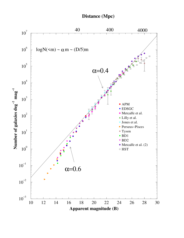
Figure 85: The galaxy number counts in the $B$-band, from several surveys. In the range $12\mathrel{\hbox to0.0pt{\lower 3.0pt\hbox{$\mathchar 536\relax$}\hss}\raise 2.0pt\hbox{$\mathchar 316\relax$}}m\mathrel{\hbox to0.0pt{\lower 3.0pt\hbox{$\mathchar 536\relax$}\hss}\raise 2.0pt\hbox{$\mathchar 316\relax$}}19$ the counts show an exponent $\alpha\approx 0.6\pm 0.1$, while in the range $19\mathrel{\hbox to0.0pt{\lower 3.0pt\hbox{$\mathchar 536\relax$}\hss}\raise 2.0pt\hbox{$\mathchar 316\relax$}}m\mathrel{\hbox to0.0pt{\lower 3.0pt\hbox{$\mathchar 536\relax$}\hss}\raise 2.0pt\hbox{$\mathchar 316\relax$}}28$ the exponent is $\alpha\approx 0.4$. The solid line is computed from the determination of the amplitude of the conditional density at small scale, the fractal dimension $D=2.2$, and from the knowledge of the luminosity function. The distance is computed for a galaxy with $M=-16$ and we have used $H_{0}=75kmsec^{-1}Mpc^{-1}$.

we have collected all the recent observations of $N(<m)$ versus $m$ in the $B$-spectral-band $m_{B}$ [125, 126, 127, 128, 129, 130, 133, 134, 137, 138, 139, 140]. At bright and intermediate magnitudes ($\>12\mathrel{\hbox to0.0pt{\lower 3.0pt\hbox{$\mathchar 536\relax$}\hss}\raise 2.0pt\hbox{$\mathchar 316\relax$}}m_{B}\mathrel{\hbox to0.0pt{\lower 3.0pt\hbox{$\mathchar 536\relax$}\hss}\raise 2.0pt\hbox{$\mathchar 316\relax$}}18$), corresponding to small redshift ($\>z<0.2$), one obtains $\>\alpha\approx 0.6$, while from $m_{B}\sim 19$ up to $m_{B}\sim 28$ the counts are well fitted by a smaller exponent with $\alpha\approx 0.4$. The usual interpretation [3, 118, 135, 136, 132, 131] is that $\alpha\approx 0.6$ corresponds to $D\approx 3$ consistent with homogeneity, while at large scales galaxy evolution and space time expansion effects are invoked to explain the lower value $\alpha\approx 0.4$. On the basis of the previous discussion of the VL samples, this interpretation is untenable. In fact, we know for sure that, at least up to $\sim 150h^{-1}Mpc$ there are fractal correlations, as we have discussed in the previous sections, so one would eventually expect the opposite behavior. Namely small value of $\alpha\approx 0.4$ (consistent with $D\approx 2$) at small scales followed by a crossover to an eventual homogeneous distribution at large scales ($\alpha\approx 0.6$ and $D\approx 3$).

The GNC in the (red) $R$-band shows an exponent $\alpha\approx 0.37-0.41$ in the range $20<R<23$ [127, 129, 125]. Moreover Gardner et al. [137] have studied the GNC in the (infrared) K-band in the range $\>12\mathrel{\hbox to0.0pt{\lower 3.0pt\hbox{$\mathchar 536\relax$}\hss}\raise 2.0pt\hbox{$\mathchar 316\relax$}}K\mathrel{\hbox to0.0pt{\lower 3.0pt\hbox{$\mathchar 536\relax$}\hss}\raise 2.0pt\hbox{$\mathchar 316\relax$}}23$, and they show that the slope of the counts changes at $K\approx 17$ from $\>0.67$ to $\>0.26$ (see also [138, 139, 140, 141]). Djorgovski et al. [142] found that the slope of the GNC is little bit higher than [137], i.e. $\alpha=0.315\pm 0.02$ between $K=20$ and $24$ mag.

The situation is therefore quite similar in the different spectral bands. The puzzling behavior of the GNC represents an important apparent contradiction we find in the data analysis. We argue here that this apparently contradictory experimental situation can be fully understood on the light of the small scale effects in the space distribution of galaxies (Sec.6). For example a fractal distribution is non analytic in every occupied point: it is not possible to define a meaningful average density because we are dealing with intrinsic fluctuations which grow with as the scale of the system itself. This situation is qualitatively different from an homogeneous picture, in which a well defined density exists, and the fluctuations represent only small amplitude perturbations. The nature of the fluctuations in these two cases is completely different, and for fractals the fluctuations themselves define all the statistical properties of the distribution. This concept has dramatic consequences in the following discussion as well as in the determination of various observable quantities, such as the amplitude of the two point angular correlation function. It is worth to notice that the small scale effects are usually neglected in the study of fractal structures because one can generate large enough (artificial) structures to avoid these problems. In Astrophysics the data are instead intrinsically limited and, as we have already mentioned in the previous two sections, a detailed analysis of finite size effects is very important. We discuss the problems of finite size effects in the determination of the asymptotic properties of fractal distributions, considering explicitly the problems induced by the lower cut-off (Sec.6).

7.2 Galaxy counts: basic relations

We briefly introduce some basic relations which are useful later. We can start by computing the expected GNC in the simplest case of a magnitude limited (ML) sample. A ML sample is obtained by measuring all the galaxies with apparent magnitude brighter than a certain limit $m_{lim}$. In this case we have (for $m<m_{lim}$)

$$N(<m)=B\Phi(\infty)10^{\frac{D}{5}m}$$ (130)

where

$$\Phi(\infty)=\int_{-\infty}^{\infty}\phi(M)10^{-\frac{D}{5}(M+25)}dM\;.$$ (131)

We consider now the case of a volume limited (VL) sample. A VL sample consists of every galaxy in the volume which is more luminous than a certain limit, so that in such a sample there is no incompleteness for an observational luminosity selection effect [18, 2]. Such a sample is defined by a certain maximum distance $R$ and an absolute magnitude limit given by:

$$M_{lim}=m_{lim}-5\log_{10}R-25-A(z)$$ (132)

($m_{lim}$ is the survey apparent magnitude limit). By performing the calculations for the number-magnitude relation, we obtain

$$N(<m)=A(m)\cdot 10^{\frac{D}{5}m}+C(m)$$ (133)

where $A(m)$ is

$$A(m)=B\int_{M(m)}^{M_{lim}}\phi(M)10^{-\frac{D}{5}(M+25)}dM$$ (134)

and $M(m)$ is given by $M(m)=m-5\log(R)-25$, and it is a function of $m$. The second term is

$$C(m)=BR^{D}\int_{-\infty}^{M(m)}\phi(M)dM\;.$$ (135)

This term, as $A(m)$, depends on the VL sample considered. We assume a luminosity function with a Schecther shape (see Sec.3). For $M(m)\mathrel{\hbox to0.0pt{\lower 3.0pt\hbox{$\mathchar 536\relax$}\hss}\raise 2.0pt\hbox{$\mathchar 318\relax$}}M^{*}$ we have that $C(m)\approx 0$, and $A(m)$ is nearly constant with $m$. This happens in particular for the deeper VL samples for which $M_{lim}\sim M^{*}$. For the less deeper VL ($M_{lim}>M^{*}$) samples these terms can be considered as a deviation from a power law behavior only for $m\rightarrow m_{lim}$. If one has $\phi(M)=\delta(M-M_{0})$ then it is simple to show that $\log(N(<m))\sim(D/5)m$ also in each VL sample.

7.3 Galaxy counts in redshift surveys

We have studied the GNC in the Perseus-Pisces redshift survey [40] in order to clarify the role of spatial inhomogeneities and finite size effects. In the previous sections we have analyzed the spatial properties of galaxy distribution in this sample by measuring the conditional (average) density and the radial density. Let us briefly summarize our main results.

When one computes the conditional average density, one indeed performs an average over all the points of the survey, as we have discussed in Sec.3. On the contrary the radial density is computed only from a single point, the origin (Sec.6). This allows us to extend the study of the spatial distribution up to very deep scales: the price to pay is that this method is strongly affected by statistical fluctuations and finite size effects. Analogously, when one computes $N(<m)$, one does not perform an average but just counts the points from the origin. As in the case of the radial density $n(r)$ also $N(<m)$ is strongly affected by statistical fluctuations due to finite size effects. as well as intrinsic oscillations that are not smoothed out. We are now able to clarify how the behavior of $N(<m)$, and in particular its exponent, are influenced by these effects.

We show in Fig.86,

Figure 86: $(a)$ The Number counts $N(<m)$ for the VL sample VL60. The slope is $\alpha\approx 0.6$. In this case occurs a flattening for $m\rightarrow m_{lim}$. $(b)$ The Number counts $N(<m)$ for the VL sample VL110. The slope is $\alpha\approx 0.4$, a part from the initial fast growth due to weak statistics. This behavior corresponds to a well defined define power law behavior of the density with exponent $D\approx 5\alpha\approx 2$.

and Fig.87

Figure 87: The Number counts $N(<m)$ for the whole magnitude limit sample. The slope is $\alpha\approx 0.6$ and it is clearly associated only to fluctuations in the spatial distribution rather than to a real homogeneity in space.

the behavior of $N(<m)$ respectively for the various VL samples and for the whole magnitude limit sample. In VL60 there are very strong inhomogeneities in the behavior of $n(r)$ (see Fig.62) and these are associated with a slope $\alpha\approx 0.6$ for the GNC. (The flattening for $m\rightarrow m_{lim}$ is just to a luminosity selection effect that is explained in Sec.7.2). For VL110 the behavior of the density is much more regular and smooth, so that it shows indeed a clear power law behavior. Correspondingly the behavior of $N(<m)$ is well fitted by $\alpha\approx 0.4$. Finally the whole magnitude limit sample is again described by an exponent $\alpha\approx 0.6$.

We have now enough elements to describe the behavior of the GNC. The first point is that the exponent of the GNC is strongly related to the space distribution. Indeed, what has never been taken into account before is the role of finite size effects [23]. The behavior of the GNC is determined by a convolution of the space density and the luminosity function, and the space density enters in the GNC as an integrated quantity. The problem is to consider the correct space density in the interpretation of data analysis. In fact, if the density has a very fluctuating behavior in a certain region of length scale, as in the case shown in Fig.62, its integral over this range of length scales is almost equivalent to a flat one. This can be seen also in Fig.61: at small distances one finds almost no galaxies because one is below the mean minimum separation between neighbor galaxies. Then the number of galaxies starts to grow, but this regime is strongly affected by finite size fluctuations. Finally the correct scaling region $r\approx\lambda$ is reached. This means for example that if one has a fractal distribution, there is first a raise of the density, due to finite size effects and characterized by strong fluctuations, because no galaxies are present before a certain characteristic scale. Once one enters in the correct scaling regime for a fractal the density becomes to decay as a power law. So in this regime of raise and fall with strong fluctuations there is a region in which the density can be approximated roughly by a constant value. This leads to an apparent exponent $D\approx 3$, so that the integrated number grows as $N(<r)\sim r^{3}$ and it is associated in terms of GNC, to $\alpha\approx 0.6$ (Fig.88).

Figure 88: The number counts $N(<m)$ in a magnitude limit sample, together with the behavior of the space density. At small scale the density is characterized by having strong fluctuations which lead to a slope $\alpha\approx 0.6$. This is clearly associated only to fluctuations in the spatial distribution rather than to a real homogeneity in space. At larger scales (faint end) the correct scaling behavior is recovered and $\alpha=D/5$.

This exponent is therefore not a real one but just due to finite size fluctuations. Only when a well defined statistical scaling regime has been reached, i.e. for $r>\lambda$, one can find the genuine scaling properties of the structure, otherwise the behavior is completely dominated by spurious finite size effects. In the VL samples where $n(r)$ scales with the asymptotic properties (Fig.86) the GNC grows also with the right exponent ($\alpha=D/5$).

If we now consider instead the behavior of the GNC in the whole magnitude limit (hereafter ML) survey, we find that the exponent is $\alpha\approx 0.6$ (Fig.87). This behavior can be understood by considering that at small distances, well inside the distance $\lambda$ defined by Eq.114, the number of galaxies present in the sample is large because there are galaxies of all magnitudes. Hence the majority of galaxies correspond to small distances ($r<\lambda$) and the distribution has not reached the scaling regime in which the statistical self-averaging properties of the system are present. For this reason in the ML sample the finite size fluctuations dominate completely the behavior of the GNC. Therefore this behavior in the ML sample is associated with spurious finite size effects rather than to real homogeneity. We discuss in a more quantitative way the behavior in ML surveys later.

7.3.1 Test on finite size effects: the averege $N(<m)$

To prove that the behavior found in Fig.87, i.e. that the exponent $\alpha\approx 0.6$ is connected to large fluctuations due to finite size effects in the space distribution and not to real homogeneity, we have done the following test. We have adopted the same procedure used for the computation of the correlation function (see Sec.3), i.e. we make an average for $N(<m)$ from all the points of the sample rather than counting it from the origin only.

To this aim we have considered a VL sample with $N$ galaxies and we have built $N$ independent flux-limited surveys in the following way. We consider each galaxy in the sample as the observer, and for each observer we have computed the apparent magnitudes of all the other galaxies. To avoid any selection effect we consider only the galaxies which lie inside a well defined volume around the observer. This volume is defined by the maximum sphere fully contained in the sample volume with the observer as a center.

Moreover we have another selection effect due to the fact that our VL sample has been built from a ML survey done with respect to the origin. To avoid this incompleteness we have assigned to each galaxy a constant magnitude $M$. In fact, our aim is to show that the inhomogeneity in the space distribution plays the fundamental role that determines the shape of the $N(<m)$ relation, and the functional form of the luminosity function enters in Eq.134 only as an overall normalizing factor.

Once we have computed $N_{i}(<m)$ from all the points $i=1,..,N$ we then compute the average. We show in Fig.89

Figure 89: Left panel The average $N(<m)$ in the VL sample VL60. The squares crosses refer to the average $N(<m)$ computed assigning to all the galaxies the same absolute magnitude $M_{0}=M^{*}$. The reference line has a slope $\alpha=0.4$. Right panel The average $N(<m)$ in the VL sample VL110. The squares crosses refer to the average $N(<m)$ computed assigning to all the galaxies the same absolute magnitude $M_{0}=M^{*}$. The reference line has a slope $\alpha=0.4$

the results for VL60 and VL110: a very well defined exponent $\alpha=D/5\approx 0.4$ is found in both cases. This is in fully agreement with the average space density (the conditional average density $\Gamma(r)$) that shows $D\approx 2$ in these VL samples.

We have also performed various tests on artificial distributions with a priori assigned properties. Using the random $\beta-$model algorithm and we have performed the analysis by assigning to each point of the system the same absolute magnitude. The results are in complete agreement with the previous findings: if we do not perform any average the exponent of the GNC is strongly affected by the presence of fluctuations due to finite size effects and we obtain $\alpha\approx 0.6$, while if we compute the GNC by making an average over all the points of the structure we find again that the relation $\alpha=D/5$ holds in a very well approximation (see [23] for more details). On the contrary in the homogeneous case one does need to perform any average to recover the correct scaling properties of $N(<m)$, because the system reaches very soon ($r\mathrel{\hbox to0.0pt{\lower 3.0pt\hbox{$\mathchar 536\relax$}\hss}\raise 2.0pt\hbox{$\mathchar 318\relax$}}\ell$) the correct scaling properties.

7.3.2 Behavior of galaxy counts in magnitude limited samples

We are now able to clarify the problem of ML catalogs. Suppose to have a certain survey characterized by a solid angle $\Omega$ and we ask the following question: up to which apparent magnitude limit $m_{lim}$ we have to push our observations to obtain that the majority of the galaxies lie in the statistically significant region ($r\mathrel{\hbox to0.0pt{\lower 3.0pt\hbox{$\mathchar 536\relax$}\hss}\raise 2.0pt\hbox{$\mathchar 318\relax$}}\lambda$) defined by Eq.114. Beyond this value of $m_{lim}$ we should recover the genuine properties of the sample because, as we have enough statistics, the finite size effects self-average. From the previous condition for each solid angle $\Omega$ we can find an apparent magnitude limit $m_{lim}$ so that finally we are able to obtain $m_{lim}=m_{lim}(\Omega)$ in the following way.

In order to clarify the situation, we can now compute the expected value of the counts if we use the approximation for the behavior of the mass-length relation given by Eqs.115-117. Suppose, for seek of clarity, also that $\phi(M)=\delta(M-M_{o})$, with $M_{o}=-19$. We define

$$\lambda=10^{0.2(m_{\lambda}-M-25)}$$ (136)

where $\lambda$ is given by Eq.114. Then the differential counts are given by

$$\left(\frac{dN}{dm}\right)_{i}=\frac{\log_{e}10}{5}3B_{1}\cdot 10^{\frac{3}{5}m}\cdot 10^{-\frac{3}{5}(M_{o}+25)}\;\;\;\mbox{if}\;\;m\mathrel{\hbox to0.0pt{\lower 3.0pt\hbox{$\mathchar 536\relax$}\hss}\raise 2.0pt\hbox{$\mathchar 316\relax$}}m_{\lambda}$$ (137)

and

$$\left(\frac{dN}{dm}\right)_{i}=\frac{\log_{e}10}{5}BD\cdot 10^{\frac{D}{5}m}\cdot 10^{-\frac{D}{5}(M_{o}+25)}\;\;\;\mbox{if}\;\;m\mathrel{\hbox to0.0pt{\lower 3.0pt\hbox{$\mathchar 536\relax$}\hss}\raise 2.0pt\hbox{$\mathchar 318\relax$}}m_{\lambda}$$ (138)

If $M_{o}=-19$ and $\lambda\sim\frac{30}{\Omega^{1/D}}(h^{-1}Mpc)$ we have

$$m_{lim}=m(\Omega)\approx 14-\frac{5}{D}\log\Omega$$ (139)

In order to give an estimate of such an effect if $\Phi(M)$ has a Schechter like shape, we can impose the condition that, in a ML sample, the peak of the selection function, which occurs at distance $r_{peak}$, satisfies the condition

$$r_{peak}>\lambda$$ (140)

where $\lambda$ in the minimal statistical length defined by Eq.114. The peak of the survey selection function occurs for $M^{*}\approx-19$ (Sec.6) and then we have $r_{peak}\approx 10^{\frac{m_{lim}-6}{5}}$. From the previous relation and from Eq.140 and Eq.114 we easily recover Eq.139.

The magnitude $m(\Omega)$ separates the $0.6$ behavior, strongly dominated by intrinsic and shot noise fluctuations, from the asymptotic $0.4$ behavior. Of course this is a crude approximation in view of the fact that $\lambda$ has not a well defined value, but it depends on the direction of observation and not only on the solid angle of the survey. However the previous equations gives a reasonable description of real data.

We show in Fig.90 the condition given by Eq.139.

Figure 90: If a survey defined by the apparent magnitude limit $m_{lim}$ and the solid angle $\Omega$ lie in the statistically significant region it is possible to obtain the self-averaging properties of the distribution also with the integral from the vertex. Otherwise one needs a redshift survey which contains the three dimensional information, and then one can perform average. Only in this way it is possible to smooth out the finite size effects.

From the previous figure it follows that for $m>19$ the statistically significant region is reached for almost any reasonable value of the survey solid angle. This implies that in deep surveys, if we have enough statistics, we readily find the right behavior ($\alpha=D/5$) while it does not happens in a self-averaging way for the nearby samples. Hence the exponent $\alpha\approx 0.4$ found in the deep surveys ($m>19$) is a genuine feature of galaxy distribution, and corresponds to real correlation properties. In the nearby surveys $m<17$ we do not find the scaling region in the ML sample for almost any reasonable value of the solid angle. Correspondingly the value of the exponent is subject to the finite size effects, and to recover the real statistical properties of the distribution one has to perform an average.

From the previous discussion it appears now clear why a change of slope is found at $m\sim 19$: this is just a reflection of the lower cut-off of the fractal structure and in the surveys with $m_{lim}>19$ the self-averaging properties of the distribution cancel out the finite size effects. This result depend very weakly on the fractal dimension $D$ and on the parameters of the luminosity function $\delta$ and $M^{*}$ used. Our conclusion is therefore that the exponent $\alpha\approx 0.4$ for $m>19$ is a genuine feature of the galaxy distribution and it is related to a fractal dimension $D\approx 2$, which is found for $m<19$ in redshift surveys only by performing averages. We note that this result is based on the assumption that the Schecther luminosity function holds also at high redshift, or, at least to $m\sim 20$. This result is confirmed by the analysis of Vettolani et al.[44] who found that the luminosity function up to $z\sim 0.2$ is in excellent agreement with that found in local surveys [37].

Finally a comment on the amplitude of counts. In Fig.85 the solid line represents the behavior of Eq.130. The prefactor $B$ has been determined as is Sec.6, while the fractal dimension is $D=2.2$. The parameter of the luminosity function are $\delta=-1.1$ and $M^{*}=-19.5$ as usual. The agreement at faint magnitudes ($m\mathrel{\hbox to0.0pt{\lower 3.0pt\hbox{$\mathchar 536\relax$}\hss}\raise 2.0pt\hbox{$\mathchar 318\relax$}}19$) is quite good. At bright magnitudes one usually underestimates the number of galaxies because of finite size effects, even in some cases the number counts can be larger than the predicted value. This is related to the asymmetry of the fluctuations in a fractal structure, as explained in Sec.6. For example we report in Fig.91 various determinations of the GNC in different regions of the sky (from [143]).

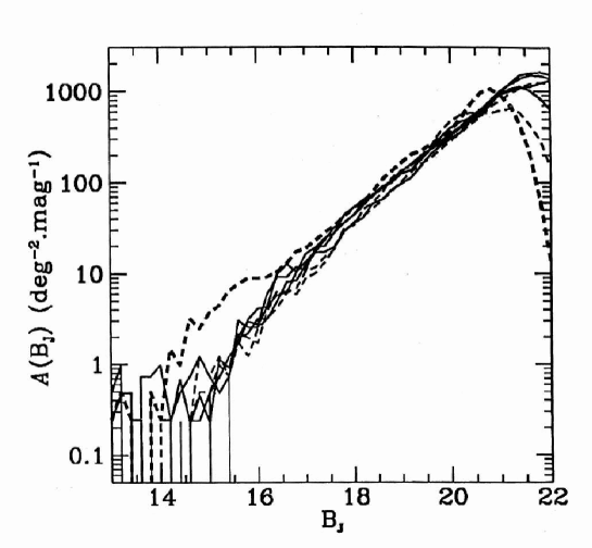
Figure 91: Determinations of the GNC in various sky regions (from Bertin & Dennefeld, 1996). The bright end wildly fluctuates around the predicted value, while at fainter magnitudes the behavior is quite smooth and is the same for the different fields.

The fact that at faint magnitudes the behavior is quite regular, is due to the smoothing of spatial fluctuations for the luminosity effect. Namely at a given apparent magnitude there are contribution from galaxies located at very different distance, as the luminosity function of galaxies is spread over several decades of luminosities (see Sec.7.5.1). On the other hand at the bright end there are contributions only from nearby galaxies, and is such a way the space finite size fluctuations are not smoothed out.

In the data shown in Fig.85 K-corrections have been not applied. Such corrections must be present because of the Hubble distance-redshift relation. Namely the spectrum of a certain galaxy at redshift $z$ is shifted towards red of a certain amount, according to the Hubble law. There are several galaxies (E/S0) with steep spectra and hence for these one detects a lower value of the intensity of the ”true” one because of the shift of the maximum of the spectrum. However there are several other galaxies (Sdm, Scd) with flat spectra. In some case the shift due to the Hubble law may produce an higher intensity while in other a decrease of the apparent flux. The K-corrections are model dependent corrections: the sign can be in both directions, i.e. towards an increasing or a decreasing of the absolute magnitude [144]. Moreover the effect of such corrections is in general not so important for the distortion of the number counts relation [135].

7.3.3 Galaxy Counts in the various spectral bands

Finally we report in Tab.8

Photometric Band	Driver	Metcalfe	Tyson	Lilly	Djorgovski	Jones
U	-	-	-	-	-	0.5
B	0.43	0.49	0.45	0.38	-	-
V	0.39	-	-	-	-	-
R	0.37	0.37	0.39	-	-	-
I	0.34	-	0.34	0.32	-	-
K	-	-	-	-	0.32	-

Table 8: The exponents of galaxy counts in different spectral bands derived by different authors.

the exponents of the galaxy counts in different frequency bands, at faint magnitudes. The faint end exponent is lower than $0.6$ in all the case, and it is in the range $0.3\div 0.5$, so that $D$ is in the range $1.5\div 2.5$. These differences can be probably related to the oscillations that may affect the behavior of the radial density as computed from a single point. In particular, as we have already discussed in Sec.6.1, in the determination of the mass-length relation from one point only (the same argument can be extended to the case of galaxy counts), there are intrinsic fluctuations that are not smoothed out by any averaging procedure. It is important to stress again that these fluctuations are proportional to the number of points, rather than to its root mean square, as in a Poisson distribution. The effect of the intrinsic fluctuations may strongly depend on the geometry of the survey, and this is why we can have different determinations of the number counts exponent, as well as fluctuations in the amplitude [113]. Only a three dimensional analysis, in which it is possible to compute average quantities, allows one to clarify the situation.

7.4 Counts of X-ray sources, Radio galaxies, Quasars and $\gamma$-ray burst sources

In observational astrophysics there are a lot of data which are only angular ones, as the measurements of distances is general a very complex task. We briefly discuss here the distribution of radiogalaxies, Quasars and the $\gamma$-ray burst distribution. Our conclusion is that all these data are compatible with a fractal structure with $D\approx 1.6\div 2.0$ similar to that of galaxies.

7.4.1 Radio galaxies

The majority of catalog radio sources are extragalactic and some of the strongest are at cosmological distances. One of the most important information on radio galaxies distribution has been obtained from the sources counts as a function of the apparent flux [145]. Extensive surveys of sources have been made at various frequencies in the range $0.4\div 5\;GHz$. In Fig.92

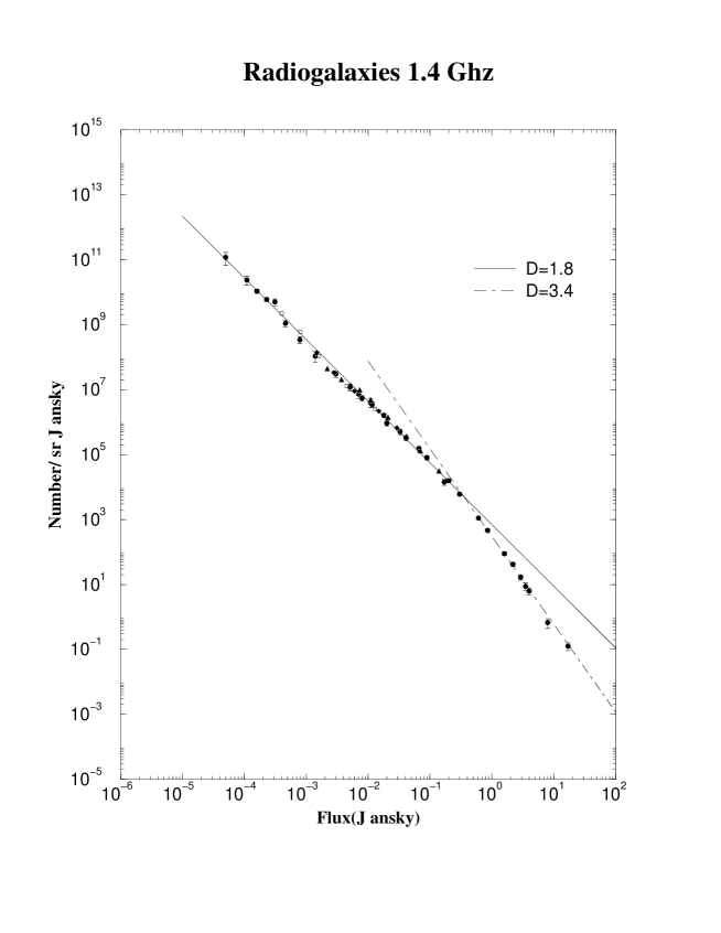
Figure 92: Normalized differential sources counts at $\nu=1.4Ghz$. Abscissa log flux density (Jy). Ordinate log differential number of sources $n(S)$. The solid line represents the behavior of a fractal structure with $D=1.8$. The amplitude has been computed from the knowledge of the luminosity function (see text). The agreement is excellent, except in the bright fluxes region due to the presence of finite size fluctuations. (From Condon, 1984).

we show a compendium of sources counts at $\nu=1.4Ghz$ [145]. The differential counts are plotted against the apparent flux. In the bright flux region there is a deviation from a power law function, while for four decades the agreement with a fractal distribution with $D\approx 1.8$ is excellent. Such a behavior has been usually explained in literature as an effect of sources/space-time evolution. Here we propose that the radio galaxies are fractally distributed, as galaxies, with almost the same fractal dimension. The deviation at bright fluxes in this picture is explained as a spurious effect due to the small scale fluctuations, as in the case of galaxy counts. In the other frequency bands the situation is nearly the same [145]. The simple picture of a fractal distribution of radio sources is therefore fully compatible with the experimental situation.

It is simple to show that the differential number of radio galaxies for unit flux (in Jansky) and unit steradian, in an Euclidean space, is given by:

$$n(S)=\frac{1}{(3\cdot 10^{9})^{2}}\left(\frac{1}{4\pi}\right)^{\frac{D+2}{2}}\frac{DB_{R}}{2}S^{-\frac{D+2}{2}}\int\phi(L)dL$$ (141)

where we have taken, as usual, $n(r)=(B_{R}D/4\pi)r^{D-3}$ and $S=L/(4\pi r^{2})$ ($L$ is the intrinsic luminosity). From the knowledge of the parameters of the luminosity function (see [145]) we have that a good approximation of the data reported in Fig.92 is given by $D=1.8$ and $B_{R}=0.1Mpc^{-D}$. Such a low value for $B_{R}$ implies that the density of radio galaxies is about 100 lower than that of optical galaxies. When it will be possible to have a complete redshift sample of Radio galaxies, i.e. a well defined volume limited sample, one will be able to measure directly $B_{R}$ and $D$ from the knowledge of the conditional density and hence to compare those values with the ones we have measured from the number flux relation.

7.4.2 Quasars

In the case of Quasars the situation is almost the same. In fact we find that at bright magnitudes ($14.75<B<18.75$) the exponent of the counts is $\alpha\approx 0.88$, while at faint magnitude it is $\alpha\approx 0.3$ [146]. A break in the integral Quasars counts has been found by [151] in the very deep ROSAT survey. This is the deepest optically identified X-ray survey yet performed. The break in the Quasar $\log N-\log S$ relation occurs at $\sim 2\cdot 10^{-14}\;erg\;cm^{-2}\;s^{-1}$ ($0.3\div 3.5$ keV), and the slope changes from $D=3$ to $D=2.07$. The break in these counts occurs at approximately the same flux as the break in the counts of X-ray sources (see Sec.7.4.3).

Even in this case we can interpret such a behavior as due to the fractal distribution in space with $D\approx 1.5\div 2$. This is a crude indication of the fractal behavior of Quasar space distribution: the data are not statistically robust as in the case of radio galaxies, and further studies are needed on the three dimensional distribution.

7.4.3 X-ray sources

The counts of X-ray sources have been measured recently by the Rosat Satellite [147]. The data are not spread over a large interval in apparent flux (about four orders of magnitude), but there is a clear evidence of a change of slope at $\sim 2.5\cdot 10^{-14}erg\;cm^{-2}\;s^{-1}$, well beyond the flux limit of the survey. Even in this case the effect of finite size fluctuations must be present and we can interpret this change of slope as an evidence of fractal distribution of the X-ray sources with dimension $D\approx 1.8$, as in the case of optical galaxies.

7.4.4 $\gamma$ ray bursts

Finally we comment the distribution of $\gamma$-ray burst (GRB). This is a long-standing problem in Astrophysics and after 20 years of intense studies and observations it is still mysterious: the origin of GRBs, in our galaxy or from the Cosmos, is a matter of debate [148, 149, 150]. We argue here that from the present angular and intensity data it is possible to show that the space distribution of $\gamma$-ray bursts sources is fully compatible with a fractal structure with $D\approx 1.7$. This result clarifies the statistical analysis of the available data and points out a fundamental aspect of the $\gamma$-ray bursts sources distribution.

From the angular catalogs recent available [152] it is possible to study three statistical quantities. The first one is the number versus apparent intensity distribution which shows a deviation from the Euclidean behavior at low fluxes [152, 153]. The second is the $V/V_{max}$ test [154] which again provides an evidence that the spatial distribution of sources is not homogeneous [153, 152]. Finally the angular distribution is isotropic within the statistical limits [155, 152] and there is not any evidence for an angular correlation or a clustering of bursts towards the galactic center or along the galactic plane of bursts [152, 156, 157, 158]. These results together indicate that the bursts sources are distributed isotropic but not homogeneously [152]. We argue here that these three evidences are fully compatible with a fractal distribution of sources with $D\approx 1.7$.

In the standard interpretation of cosmological origin of $\gamma$ ray bursts, the sources must be at very high redshift. In such a way, due to the modification of the Euclidean Geometry in the Friedmann models, one should obtain a deviation from the purely $-3/2$ behavior for the counts. However the problem is that the sources must be of very high intrinsic energy, if they are at so large distances. This seems to be the most important problem for a cosmological origin of such sources. We show that the sources can be at low redshift (say $z\mathrel{\hbox to0.0pt{\lower 3.0pt\hbox{$\mathchar 536\relax$}\hss}\raise 2.0pt\hbox{$\mathchar 316\relax$}}1$), giving the new interpretation of the counts relation.

The first observational evidence is the number of burst as a function of the apparent flux $N(>S)$. At bright apparent flux, which are associated to small distance of the sources, one sees an exponent $-3/2$, which seems to be in agreement with the homogeneous case. This is just a spurious effect which arises form the fact this quantity is computed without performing any average. At faint apparent fluxed, one is integrating the density in the correct scaling regime, and in this region the genuine statistical properties of the system can be detected. From the $N(>S)$ relation in the limit of low $S$ we can estimate a fractal dimension $D\approx 1.7\pm 0.1$. An equivalent test on the homogeneity versus fractal properties is given by the $V/V_{max}$ distribution [154], where

$$\frac{V}{V_{max}}=\left(\frac{C}{C_{lim}}\right)^{-\frac{3}{2}}\;.$$ (142)

In this ratio $V$ is the volume contained in a sphere extending to the location bursts and $V_{max}$ is the volume of the sphere extending to the maximum distance at which the same burst would be detectable by the instrument, whose limiting flux is $C_{lim}$. It is simple to show that if the spatial distribution of sources is described by a fractal structure, then we have

$$<\frac{V}{V_{max}}>=\frac{D}{D+3}$$ (143)

Even in this case the data show [152] that $<\frac{V}{V_{max}}>=0.33\pm 0.01$ which in terms of fractal dimension means $D\approx 1.5\pm 0.1$. This value is somewhat smaller than the fractal dimension estimated with the $N(>S)$. This difference is probably due to the fact that this test is integrated while the $N(>S)$ is a differential one.

Let us came to the third evidence, i.e. a substantially isotropic angular distribution and a lack of any correlation at small angles. The projection of a fractal distribution on the unit sphere conserves the correlations properties (see Sec.7.5 ) only in the small angles approximation, while at large angular scale the long range correlation are destroyed by projection effects. The angular correlation function $\omega(\theta)$ has a power law behavior in the small angles approximation ($\theta<10^{\circ}$). In the available sample [152] the number of points is $N=1122$ distributed over the whole sky. This means that at angular distance smaller than $\sim 20^{\circ}$ one does not find any other object in average, and therefore it is not possible to study the angular correlation function at such low angular separation.

These results indicate together that the $\gamma$-ray burst sources are fractally distributed in space with $D\approx 1.7$. This is value is very similar to that the fractal dimension of the galaxy distribution is space which is $D\approx 2$ up to some hundreds Megaparsec. This ”coincidence” can be seen as an indication that the $\gamma$-ray bursts sources are associate to a population of objects distributed as the visible galaxies. These objects should have low redshift, and distance up to some hundreds Megaparsec, depending on the intrinsic luminosity of the sources. We stress that recently a correlation between the $\gamma$ ray bursts at the 3B catalog and the Abell clusters has been found [159]. This evidence points towards a cosmological origin of bursts, and can be in agreement with our interpretation of the counts distribution. In fact, the sample of bursts considered are located within $\sim 600h^{-1}Mpc$ [159] where the modification of the Euclidean Geometry are negligible.

We stress that a larger sample of bursts may allow one a better determination of the fractal dimension and, if the number of objects for steradian will became larger, it may be possible to study also the angular correlations in the small angle approximation.

7.4.5 Compendium of counts

In Tab.9 we summarize the behavior of the number counts for various astrophysical objects. The small scale exponent corresponds to the bright end of the number counts relation, while the large scale exponent to the faint end. The ”small scale exponent” is not a real exponent and wildly fluctuates for the different objects. On the contrary the large scale exponent is a real exponent and its value is in the range $1.8\mathrel{\hbox to0.0pt{\lower 3.0pt\hbox{$\mathchar 536\relax$}\hss}\raise 2.0pt\hbox{$\mathchar 316\relax$}}D\mathrel{\hbox to0.0pt{\lower 3.0pt\hbox{$\mathchar 536\relax$}\hss}\raise 2.0pt\hbox{$\mathchar 316\relax$}}2.2$ for almost all the cases. The counts of all these different objects is therefore compatible with a fractal distribution in space.

This implies a completely new interpretation of the counts. At small scale the exponent $D\approx 3$ (i.e $\alpha\approx 0.6$ in the case of magnitude counts) is due to finite size effects and not to a real homogeneity: this has be shown to be the case with very specific tests. On the other hand, at larger scale the value $D\approx 2$ (i.e. $\alpha\approx 0.4$) corresponds to the correct correlation properties of the samples, that we can find by the complete correlation analysis in the three dimensional space. This implies that galaxy evolution, modifications of the Euclidean Geometry and the K-corrections are not very relevant in the range of the present data. In addition the fact that the exponent $\alpha\approx 0.4$ holds up to magnitude $27\div 28$ for galaxies seems to indicate that the fractal may continue up to distances $\sim 4000h^{-1}Mpc$. Quite a remarkable fact if one considers that the Hubble radius of the Universe is supposed to be $4000h^{-1}Mpc$. Moreover such a behavior can be found for galaxies in the different photometric bands, as well as for other astrophysical objects.

Objects	Small scale behavior		Large scale behavior
U-band1	$?\mathrel{\hbox to0.0pt{\lower 3.0pt\hbox{$\mathchar 536\relax$}\hss}\raise 2.0pt\hbox{$\mathchar 316\relax$}}U\mathrel{\hbox to0.0pt{\lower 3.0pt\hbox{$\mathchar 536\relax$}\hss}\raise 2.0pt\hbox{$\mathchar 316\relax$}}18$	$D\approx?$	$18\mathrel{\hbox to0.0pt{\lower 3.0pt\hbox{$\mathchar 536\relax$}\hss}\raise 2.0pt\hbox{$\mathchar 316\relax$}}U\mathrel{\hbox to0.0pt{\lower 3.0pt\hbox{$\mathchar 536\relax$}\hss}\raise 2.0pt\hbox{$\mathchar 316\relax$}}24$	$D\approx 2.5$
B-band2	$12\mathrel{\hbox to0.0pt{\lower 3.0pt\hbox{$\mathchar 536\relax$}\hss}\raise 2.0pt\hbox{$\mathchar 316\relax$}}B\mathrel{\hbox to0.0pt{\lower 3.0pt\hbox{$\mathchar 536\relax$}\hss}\raise 2.0pt\hbox{$\mathchar 316\relax$}}18$	$D\approx 3$	$18\mathrel{\hbox to0.0pt{\lower 3.0pt\hbox{$\mathchar 536\relax$}\hss}\raise 2.0pt\hbox{$\mathchar 316\relax$}}B\mathrel{\hbox to0.0pt{\lower 3.0pt\hbox{$\mathchar 536\relax$}\hss}\raise 2.0pt\hbox{$\mathchar 316\relax$}}28$	$D\approx 2$
V-band3	$\mathrel{\hbox to0.0pt{\lower 3.0pt\hbox{$\mathchar 536\relax$}\hss}\raise 2.0pt\hbox{$\mathchar 316\relax$}}20$	$D\approx?$	$22\mathrel{\hbox to0.0pt{\lower 3.0pt\hbox{$\mathchar 536\relax$}\hss}\raise 2.0pt\hbox{$\mathchar 316\relax$}}V\mathrel{\hbox to0.0pt{\lower 3.0pt\hbox{$\mathchar 536\relax$}\hss}\raise 2.0pt\hbox{$\mathchar 316\relax$}}25$	$D\approx 1.95$
R-band4	$15\mathrel{\hbox to0.0pt{\lower 3.0pt\hbox{$\mathchar 536\relax$}\hss}\raise 2.0pt\hbox{$\mathchar 316\relax$}}R\mathrel{\hbox to0.0pt{\lower 3.0pt\hbox{$\mathchar 536\relax$}\hss}\raise 2.0pt\hbox{$\mathchar 316\relax$}}18$	$D\approx 2.8$	$20\mathrel{\hbox to0.0pt{\lower 3.0pt\hbox{$\mathchar 536\relax$}\hss}\raise 2.0pt\hbox{$\mathchar 316\relax$}}R\mathrel{\hbox to0.0pt{\lower 3.0pt\hbox{$\mathchar 536\relax$}\hss}\raise 2.0pt\hbox{$\mathchar 316\relax$}}26$	$D\approx 1.85$
I-band5	$?\mathrel{\hbox to0.0pt{\lower 3.0pt\hbox{$\mathchar 536\relax$}\hss}\raise 2.0pt\hbox{$\mathchar 316\relax$}}I\mathrel{\hbox to0.0pt{\lower 3.0pt\hbox{$\mathchar 536\relax$}\hss}\raise 2.0pt\hbox{$\mathchar 316\relax$}}19$	$D\approx?$	$19\mathrel{\hbox to0.0pt{\lower 3.0pt\hbox{$\mathchar 536\relax$}\hss}\raise 2.0pt\hbox{$\mathchar 316\relax$}}I\mathrel{\hbox to0.0pt{\lower 3.0pt\hbox{$\mathchar 536\relax$}\hss}\raise 2.0pt\hbox{$\mathchar 316\relax$}}25$	$D\approx 1.7$
K-band6	$12\mathrel{\hbox to0.0pt{\lower 3.0pt\hbox{$\mathchar 536\relax$}\hss}\raise 2.0pt\hbox{$\mathchar 316\relax$}}K\mathrel{\hbox to0.0pt{\lower 3.0pt\hbox{$\mathchar 536\relax$}\hss}\raise 2.0pt\hbox{$\mathchar 316\relax$}}17$	$D\approx 3.35$	$20\mathrel{\hbox to0.0pt{\lower 3.0pt\hbox{$\mathchar 536\relax$}\hss}\raise 2.0pt\hbox{$\mathchar 316\relax$}}K\mathrel{\hbox to0.0pt{\lower 3.0pt\hbox{$\mathchar 536\relax$}\hss}\raise 2.0pt\hbox{$\mathchar 316\relax$}}24$	$D\approx 1.6$
Quasars7	$14.75\mathrel{\hbox to0.0pt{\lower 3.0pt\hbox{$\mathchar 536\relax$}\hss}\raise 2.0pt\hbox{$\mathchar 316\relax$}}B\mathrel{\hbox to0.0pt{\lower 3.0pt\hbox{$\mathchar 536\relax$}\hss}\raise 2.0pt\hbox{$\mathchar 316\relax$}}18.75$	$D\approx 4.4$	$19\mathrel{\hbox to0.0pt{\lower 3.0pt\hbox{$\mathchar 536\relax$}\hss}\raise 2.0pt\hbox{$\mathchar 316\relax$}}B\mathrel{\hbox to0.0pt{\lower 3.0pt\hbox{$\mathchar 536\relax$}\hss}\raise 2.0pt\hbox{$\mathchar 316\relax$}}23$	$D\approx 1.5$
Radio8 $\nu=1.4Ghz$	$1\mathrel{\hbox to0.0pt{\lower 3.0pt\hbox{$\mathchar 536\relax$}\hss}\raise 2.0pt\hbox{$\mathchar 316\relax$}}S\mathrel{\hbox to0.0pt{\lower 3.0pt\hbox{$\mathchar 536\relax$}\hss}\raise 2.0pt\hbox{$\mathchar 316\relax$}}10$	$D\approx 3.44$	$10^{-5}\mathrel{\hbox to0.0pt{\lower 3.0pt\hbox{$\mathchar 536\relax$}\hss}\raise 2.0pt\hbox{$\mathchar 316\relax$}}S\mathrel{\hbox to0.0pt{\lower 3.0pt\hbox{$\mathchar 536\relax$}\hss}\raise 2.0pt\hbox{$\mathchar 316\relax$}}1$	$D\approx 1.8$
Radio8 $\nu=0.61Ghz$	$1\mathrel{\hbox to0.0pt{\lower 3.0pt\hbox{$\mathchar 536\relax$}\hss}\raise 2.0pt\hbox{$\mathchar 316\relax$}}S\mathrel{\hbox to0.0pt{\lower 3.0pt\hbox{$\mathchar 536\relax$}\hss}\raise 2.0pt\hbox{$\mathchar 316\relax$}}10$	$D\approx 3.8$	$10^{-3}\mathrel{\hbox to0.0pt{\lower 3.0pt\hbox{$\mathchar 536\relax$}\hss}\raise 2.0pt\hbox{$\mathchar 316\relax$}}S\mathrel{\hbox to0.0pt{\lower 3.0pt\hbox{$\mathchar 536\relax$}\hss}\raise 2.0pt\hbox{$\mathchar 316\relax$}}1$	$D\approx 1.6$
Radio8 $\nu=0.408Ghz$	$1\mathrel{\hbox to0.0pt{\lower 3.0pt\hbox{$\mathchar 536\relax$}\hss}\raise 2.0pt\hbox{$\mathchar 316\relax$}}S\mathrel{\hbox to0.0pt{\lower 3.0pt\hbox{$\mathchar 536\relax$}\hss}\raise 2.0pt\hbox{$\mathchar 316\relax$}}10$	$D\approx 3.7$	$10^{-3}\mathrel{\hbox to0.0pt{\lower 3.0pt\hbox{$\mathchar 536\relax$}\hss}\raise 2.0pt\hbox{$\mathchar 316\relax$}}S\mathrel{\hbox to0.0pt{\lower 3.0pt\hbox{$\mathchar 536\relax$}\hss}\raise 2.0pt\hbox{$\mathchar 316\relax$}}1$	$D\approx 1.5$
Radio8 $\nu=5.0Ghz$	$1\mathrel{\hbox to0.0pt{\lower 3.0pt\hbox{$\mathchar 536\relax$}\hss}\raise 2.0pt\hbox{$\mathchar 316\relax$}}S\mathrel{\hbox to0.0pt{\lower 3.0pt\hbox{$\mathchar 536\relax$}\hss}\raise 2.0pt\hbox{$\mathchar 316\relax$}}10$	$D\approx 3.4$	$10^{-4}\mathrel{\hbox to0.0pt{\lower 3.0pt\hbox{$\mathchar 536\relax$}\hss}\raise 2.0pt\hbox{$\mathchar 316\relax$}}S\mathrel{\hbox to0.0pt{\lower 3.0pt\hbox{$\mathchar 536\relax$}\hss}\raise 2.0pt\hbox{$\mathchar 316\relax$}}1$	$D\approx 1.8$
X-ray sources9	$5\cdot 10^{-13}\mathrel{\hbox to0.0pt{\lower 3.0pt\hbox{$\mathchar 536\relax$}\hss}\raise 2.0pt\hbox{$\mathchar 316\relax$}}S\mathrel{\hbox to0.0pt{\lower 3.0pt\hbox{$\mathchar 536\relax$}\hss}\raise 2.0pt\hbox{$\mathchar 316\relax$}}10^{-12}$	$D\approx 3.4$	$10^{-16}\mathrel{\hbox to0.0pt{\lower 3.0pt\hbox{$\mathchar 536\relax$}\hss}\raise 2.0pt\hbox{$\mathchar 316\relax$}}S\mathrel{\hbox to0.0pt{\lower 3.0pt\hbox{$\mathchar 536\relax$}\hss}\raise 2.0pt\hbox{$\mathchar 316\relax$}}5\cdot 10^{-13}$	$D\approx 1.8$
$\gamma-ray$ bursts 10	$10\mathrel{\hbox to0.0pt{\lower 3.0pt\hbox{$\mathchar 536\relax$}\hss}\raise 2.0pt\hbox{$\mathchar 316\relax$}}S\mathrel{\hbox to0.0pt{\lower 3.0pt\hbox{$\mathchar 536\relax$}\hss}\raise 2.0pt\hbox{$\mathchar 316\relax$}}100$	$D\approx 3$	$10^{-1}\mathrel{\hbox to0.0pt{\lower 3.0pt\hbox{$\mathchar 536\relax$}\hss}\raise 2.0pt\hbox{$\mathchar 316\relax$}}S\mathrel{\hbox to0.0pt{\lower 3.0pt\hbox{$\mathchar 536\relax$}\hss}\raise 2.0pt\hbox{$\mathchar 316\relax$}}10$	$D\approx 1.7$

Table 9: The exponents of counts for different kinds of astrophysical objects (see text). (Ref.1-6: see Table 8; Ref.7: Hartwick & Schade, 1990; Ref.8: Condon,1984; Ref.9: Hasinger et al., 1993; Ref.10: Meegan et al.1995)

7.5 Discussion of the angular correlations and their reinterpretation

We have now enough elements to give the correct reinterpretation also of the angular catalogs. These catalogs are quantitatively inferior to the 3-d ones because they correspond to the angular projection and do not contain the third coordinate. However, the fact that they contains more galaxies with respect to the 3-d catalog has led some authors to assign an excessive importance to these catalogs and, again, they are supposed to show the much sought homogeneity. Actually the interpretation of the angular catalogs is quite delicate and ambiguous for a variety of reasons which are usually neglected.

7.5.1 Angular properties of three dimensional samples

In Fig.93

Figure 93: Angular distribution (Flamsteed projection) of the various redshift surveys presented in this review.

we show the angular projection of the various redshift samples we have discussed. No large voids are present in the angular distribution, which appears quite uniform. The problem we address in what follows concerns the origin of the angular homogeneity, which appears in contradiction with the irregular three dimensional space properties.

The standard method used to analyze angular catalogs, is based on the assumption that galaxies are correlated only at small distances. In such a way the effect of the large spatial inhomogeneities is not considered at all. Under this assumption, that is not supported by any experimental evidence, it is possible to derive the Limber equation [27, 28]. In practice, the angular analysis is performed by computing the two point correlation function

$$\omega(\theta)=\frac{\langle n(\theta_{0})n(\theta_{0}+\theta)\rangle}{\langle n\rangle}-1$$ (144)

where $\langle n\rangle$ is the average density in the survey. This function is the analogous of the $\xi(r)$ for the 3-d analysis. The results of such an analysis are quite similar to the three dimensional ones [25, 3]. In particular, it has been obtained that, in the limit of small angles,

$$\omega(\theta)\sim\theta^{-\gamma+1}$$ (145)

with $\gamma\approx 1.7$ (i.e. $\gamma_{a}=\gamma-1=0.7$). It is possible to show [25] that, in the Limber approximation Eq.145, the angular correlation function corresponds to $\xi(r)\sim r^{-\gamma}$ for its three dimensional counterpart (in the case $\gamma>1$).

We now study the case of a self-similar angular distribution so that, if such properties are present in real catalogs, we are able to recognize them correctly. Of course, if the distribution is homogenous, we are able to reproduce the same results obtained by the $\omega(\theta)$ analysis. Hereafter we consider the case of small angles ($\theta\mathrel{\hbox to0.0pt{\lower 3.0pt\hbox{$\mathchar 536\relax$}\hss}\raise 2.0pt\hbox{$\mathchar 316\relax$}}1$), that is quite good the for the catalogs investigated so far. The theorem for orthogonal projections discussed in Sec.2 can be extended to the case of angular projections in the limit of small angles ($\theta<1$). Therefore in the following in Eq.31 we have $D^{\prime}=D_{a}$

In this case the number of points up to an angle $\theta$ scales as

$$N(\theta)=B_{a}\theta^{D_{a}}$$ (146)

where $D_{a}$ is the fractal dimension corresponding to the angular projection and $B_{a}$ is the lower cut-off of the distribution. Eq.146 holds from every occupied point, and in the case of an homogenous distribution we have $D_{a}=2$. Following Coleman & Pietronero [2] we define the conditional average density as

$$\Gamma(\theta)=\frac{1}{S(\theta)}\frac{dN(\theta)}{d\theta}=\frac{BD_{a}}{2\pi}\theta^{-\gamma_{a}}$$ (147)

where $S(\theta)$ is the differential solid angle element and $\gamma_{a}=2-D_{a}$ is the angular correlation exponent (angular codimension). The last equality holds in the limit $\theta<1$. From the very definition of $\Gamma(\theta)$ we have that

$$\omega(\theta)=\frac{\Gamma(\theta)}{\langle n\rangle}-1\;.$$ (148)

A first important consequence of eq.148 is that if $\Gamma(\theta)$ has a power law behavior, while $\omega(\theta)$ is a power law minus one. This corresponds to a break in the log-log plot for angular scales such that $\omega(\theta)\mathrel{\hbox to0.0pt{\lower 3.0pt\hbox{$\mathchar 536\relax$}\hss}\raise 2.0pt\hbox{$\mathchar 316\relax$}}1$. We show in Fig.94 the behaviour of such a quantity.

Figure 94: In this figure we show the behaviour of $\omega(\theta)$ (dotted line) is the case of a fractal structure with $D_{a}=1.85$ ($\gamma_{a}=0.15)$. It can be seen that the exponent obtained by fitting this function with a power law behavior (solid line) is higher than the real one ($\gamma=-0.65$). Also the break in the power law behaviour is completely artificial.

The codimension found by fitting $\omega(\theta)$ with a power law function is higher than the real one. This is an important effect that has never been considered before. As we show below, this is actually the case for real catalogs. The second important point is that the break of $\omega(\theta)$ in the log-log plot is clearly artificial and does not correspond to any characteristic scale of the original distribution. The problem is that in the case of a scale-invariant distribution the average density in Eq.144 is not well defined, as it depends on the sample size [2].

We have studied the angular conditional density in the various magnitude limited samples. The results are shown in Fig.95 Fig.96 Fig.97 and Fig.98.

Figure 95: Angular correlation function $\Gamma(\theta)$ for the magnitude limited samples LEDA14.5 and LEDA16 (North and South). The reference line has a slope $-\gamma_{a}=-0.2$ which corresponds to a fractal dimension $D=1.8$ in the 3-d space. The flattening at large angular separations is due to projection effects and does not correspond to any real feature of the 3-d distribution.

In the case of $D<2$ the exponent of the angular correlation function is expected to be $-\gamma_{a}=D-2$ [3], i.e.

$$\Gamma(\theta)\sim\theta^{-\gamma_{a}}$$ (149)

Figure 96: Angular correlation function $\Gamma(\theta)$ for the various VL samples (PP18, PP19, and PP20) and for the whole ML catalog (PPML) of Perseus-Pisces. The solid line has a slope $-\gamma_{a}=-0.2$, while the dotted line has a slope $-\gamma_{a}=-0.4$.

Figure 97: Angular correlation function $\Gamma(\theta)$ for the various VL samples (CfA1-18, CfA1-19, and CfA1-20) and for the whole ML catalog (CfA1-ML) of CfA1. The solid line has a slope $-\gamma_{a}=-0.2$, while the dotted line has a slope $-\gamma_{a}=-0.4$.

Figure 98: Angular correlation function $\Gamma(\theta)$ for the various VL samples (SS40, SS60 and SS80) and for the whole ML catalog (SSML) of SSRS1. The solid line has a slope $-\gamma_{a}=-0.4$, while the dotted line has a slope $-\gamma_{a}=-0.2$.

According to the theorem discussed in Sec.2.2.4 the orthogonal projection of a fractal structure with dimension $D$ in the $d=3$ Euclidean space, has dimension $D-2$, i.e. it should be compact for $D\geq 2$. The angular projection is different from the orthogonal one for the following reason. In the projection of at 3-d distribution on a planar infinitesimal area $dA$, we have contribution, up to the distance $R$, from a volume which growths as $dV=dA\cdot R$. On the other hand, in the projection on a infinitesimal solid angle $d\Omega$ we have contribution, up to $R$, from a 3-d volume $dV=d\Omega\cdot R^{3}$. While in the first case the number of points which contribute to the projection growths as $N_{ort}\sim R^{D-2}$, in the second case $N_{ang}\sim R^{D}$. The qualitatively difference behavior of the number of points in these two case, is one of the reason of the uniformity of angular distribution.

Although we have measured that the fractal dimension in the three dimensional Euclidean space is $D=2$, the angular correlation exponent is $-\gamma_{a}\approx-0.2$. This can be due to the fact that the result $-\gamma_{a}=D-2$ is valid in the limit of an asymptotic fractal structure, i.e. if the volume of the three dimensional sample goes to infinity. The finite size effect, due to the fact that the observed three dimensional volume is limited, can lead to a higher absolute value for the angular correlation exponent. The reason is essentially the following. We can approximate a limited fractal distribution in 3-d, as the intersection of the asymptotic 3-d structure with a plane, with a certain fixed thickness, which has dimension $d=2$. If the thickness of the plane is small enough, the resulting distribution has dimension $D_{i}=D+2-3\approx D-1\approx 1$ in the 3-d space. The angular projection of a structure with $D_{i}\approx 1$ has still dimension $1$. Hence, in this case, the angular correlation exponent is $-\gamma_{a}\approx-1$ rather than $\gamma_{a}=0$ which corresponds to the limit of having a 3-d sample extended enough.

In order to test that this is the case we have cut various catalogs at progressively smaller distances, finding that the angular correlation exponent is higher (in absolute value) as the three dimensional sample is limited in distance (see Fig.99 and Fig.100).

Figure 99: Angular correlation function $\Gamma(\theta)$ for the ML catalog LEDA-14.5, cut at $r<60h^{-1}Mpc$ and $r<30h^{-1}Mpc$. It is clearly shown the difference in the correlation exponent.

Figure 100: Angular correlation function $\Gamma(\theta)$ for ML Perseus-Pisces catalog cut at difference distances. It is clearly shown the difference in the correlation exponent. The solid line has a slope $-\gamma_{a}=-0.2$, while the dotted line has a slope $-\gamma_{a}=-0.4$.

In other words when the thickness of the 3-d sample is some few $h^{-1}Mpc$ ($\sim 20\div 40$), the angular correlation function shows a trend $-\gamma_{a}\rightarrow-1$. Otherwise when the thickness is $\sim 100h^{-1}Mpc$ or more, we get $\gamma_{a}\rightarrow 0$. As the galaxies which contribute to the angular projection are located in a large volume of space, due the mix of different length scales, the projection appears quite uniform (i.e. $\gamma_{a}\sim 0$). As shown in Fig.95 the angular correlation function presents a flattening at large angles. Such a behavior is completely spurious as the three dimensional sample is a piece of fractal up to its limiting distance. This is due to the fact that the angular catalogs are qualitatively inferior to the three dimensional ones because they do not contain the third coordinate, even if they usually contain more galaxies. Angular projections, which are magnitude limited, mix different length scales and this gives an artificial randomization of the galaxies. This implies that the angular projection of a fractal is really homogeneous at relatively large angles. Clearly this is an artificial effect and from a smooth angular projection one cannot deduce whether the real distribution is also smooth. For a detailed discussion of the scaling of the angular correlation amplitude, as well as other effects of angular projection, we refer the reader to [160, 2].

7.5.2 The large angles problem: angular projection of fractal structures

Dogterom & Pietronero [160] (see also [2]) studied the surprising and subtle properties of the angular projection of a fractal distribution. They find that the angular projection produces an artificial crossover towards homogenization with respect to the angular density. This crossover is artificial (just due to the projection) as it does not correspond to any physical features of the three dimensional distribution. Moreover they showed that there is an explicit dependence of the angular two point correlation function $\omega(\theta)$ on $\theta_{M}$ the sample angle: this effect has never been taken into account in the discussion of real angular catalogs. These arguments show that it is very dangerous to make any definite conclusion just from the knowledge of the angular distribution. By the way this is the reason why one has to measure redshifts, which, of course, is not an easy task.

However, there is a point of the discussion which remains still open. In fact, some authors [3, 29] claim that one of the most important facts that disprove the existence of fractal correlations at large scales, is the scaling of the amplitude of the two point angular correlation function (ACF) with sample depth, in the small angles approximation. We can now clarify this puzzling situation.

Before considering the problem of the angular correlation function, let us consider the angular projection of an artificial fractal. Some authors (e.g. Peebles [3]) pointed out that a fractal with dimension $D$ significantly less than three cannot approximat the observed isotropic angular distributions of deep samples. In particular Peebles [102] showed that a fractal with dimension $D\approx 2$ has large-scale angular fluctuations which are not compatible with the observed angular maps. We stress that there are various problems, which are usually neglected (e.g. [102]) in constructing an artificial distribution with the properties of the real one:

• The first point is that in generating an artificial fractal structure a very important role is played by lacunarity. As we have seen in Sec.2 and Sec.5., even if the fractal dimension is fixed, one can have very different angular distributions depending on the value of the lacunarity. In fact, if lacunarity is large, and the sample is characterized by having voids of the order of the sample size, it is clear that the angular distribution is highly inhomogeneous. On the other hand, if lacunarity is small (with respect to the sample size) one can obtain more uniform angular projections (see Fig.7). A low value of the lacunarity should therefore be used for the reproducing galaxy distribution, because the real galaxy distribution has indeed a low value of the lacunarity: in the available samples, the dimension voids is smaller than the survey volume [78]. (See [162] for more details).

• The second important point which should be considered is that the real angular distributions are magnitude limited ones, i.e. contains all the galaxies with apparent magnitudes brighter than a certain limit $m_{lim}$. This implies a mixing of length scales due to the fact that galaxies have a very spread luminosity function, and their absolute luminosity can change of more than a factor ten. For example suppose that $m_{lim}=14$, then one gets contributions from galaxies in the range of distances $\sim 1.5\div 50h^{-1}Mpc$ (see Fig.101).

  

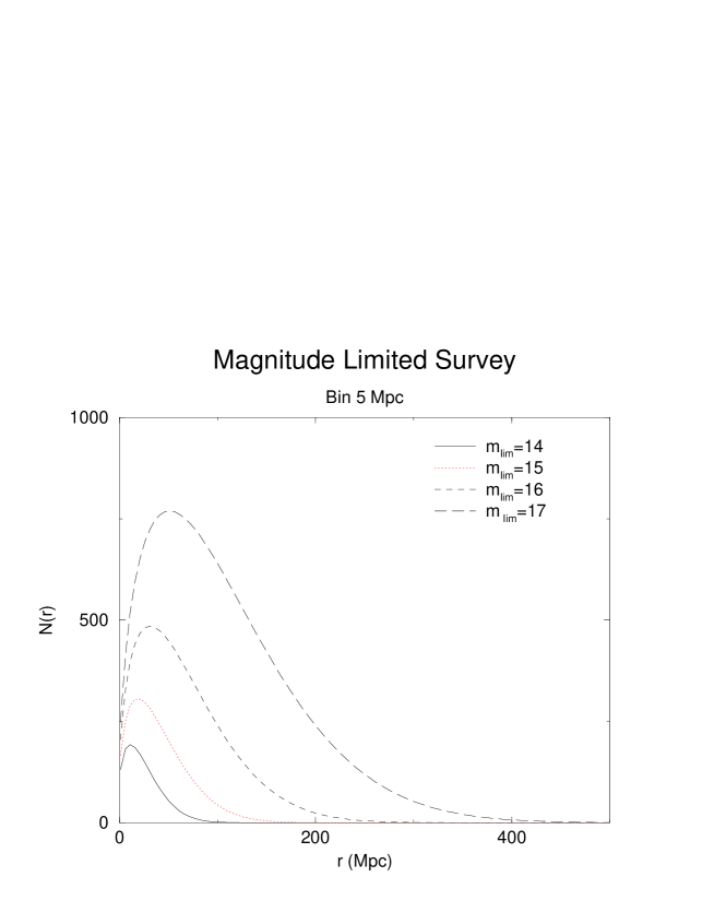
  Figure 101: Number of galaxies (per bin of $5h^{-1}Mpc$) for magnitude limited samples with different limit $m_{lim}$. As the apparent magnitude limit increases the number of galaxies at large distance, which contributes to the magnitude limit angular sample, growths. This is the origin of the mixing of luminosity and space distributions which leads to an apparent homogeneous behavior for the angular distribution

  However if, for example, $m_{lim}=17$ then the range of distances from which one has important contributions to the angular distribution, rapidly grows. This implies that galaxies in angular catalogs correspond to extremely different distances. Correspondingly the projection is a complex convolution of various luminosities and distances. This is another important reason why if one looks an angular map limited at galaxies with apparent magnitude brighter than $14$ one sees large scale fluctuations. On the other hand a catalog (as the angular APM catalog) limited at $m_{lim}>18$, is quite smoother, because the mixing of length scales is large.

• An important point, recently pointed out by Durrer et al.[162], is the following. The angular lacunarity of a 3-d fractal set with $D\approx 2$ can be very small, even if there are large voids in the space distribution. Moreover the angular fluctuations depend on whether the galaxies are projected with apparent or fixes size, being more uniform in the latter case.

7.5.3 Rescaling of the amplitude of $\omega(\theta)$

Assuming that the fractal correlation are only present at small scales, i.e. that $\xi(r)=(r_{0}/r)^{\gamma}$, it is possible to show that, if $\gamma>1$, in the small angle approximation ($\theta<<1$) one has for the homogeneous case that [3]

$$\omega(\theta)\sim\theta^{1-\gamma}(r_{0}/D_{*})^{\gamma}$$ (150)

where the depth $D_{*}$ is

$$D_{*}=\left(\frac{L_{*}}{4\pi f}\right)^{1/2}.$$ (151)

$L_{*}$ is the cut-off of the Schecther luminosity function and $f$ is the limiting flux density of the survey. In the case of a fractal distribution with $D<2$ it is easy to show that instead of Eq.150 we have [3]

$$\omega(\theta)\sim\theta^{1-\gamma}$$ (152)

so that the difference between the homogeneous and the fractal case is that in the first case the amplitude of the ACF depends on the sample depth $D_{*}$ while in the second case it is constant. Peebles [3] claims that, since in the real angular catalogs one observes the scaling of the amplitude [29, 161], this provides an evidence against the fractal behavior. We show now that this conclusion is not correct because it does not take into account the finite size effects in real galaxy surveys, as it is the case of the GNC.

In fact, the amplitude of the ACF is strongly related to the behavior of the angular number density, i.e. to $N(<m)$. Eq. 152 is obtained under the assumption that the density for a fractal scales as $r^{-\gamma}$: this is true for the average conditional density in the case of an ideal fractal distribution, if the correct scaling regime is reached. As previously discussed, the conditional density computed from a single point is instead strongly affected by finite size effects up to the characteristic minimal statistical length $\lambda$.

In order to illustrate this point we present the analysis of the ACF for the Perseus-Pisces redshift survey [40]. In Fig.102

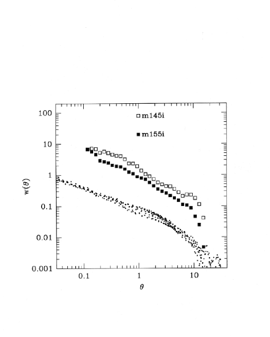
Figure 102: The angular correlation function for Peruses Pisces limited at $m_{lim}14.,5$ ($m145i$) and $15.5$ ($m155i$). The points refers to different samples of the APM catalog scaled to the ACF of the Lick survey (Maddox et al., 1990). The scaling with depth of the amplitude of the angular correlation function in this case is due to a finite size effects and it is not a proof of homogeneity in space, as we know from the space analysis that this sample has fractal behavior up to its deeper depth.

we show the behavior of the ACF $\omega(\theta)$ for the whole ML survey. There is a clear scaling of the amplitude with the apparent magnitude limit of the survey ($m_{lim}=14.5,15.5$ respectively). We know from the space analysis that the galaxy distribution is fractal in this sample and therefore this trend is not a consequence of homogeneity, but only of the finite size effects which are especially large for the counting from the vertex.

In summary the apparent homogeneity inferred from the behavior of the angular correlation amplitude as a function of depth, has the same origin as the exponent $\alpha\approx 0.6$ of the galaxy counts at bright magnitudes (small scales). Both arise from finite size effects (for a more detailed study on the ACF we refer the reader to [163]) and do not correspond to the real statistical properties.

8 Luminosity and space distributions

In a well-known review on the galaxy luminosity function (LF) Binggeli et al.[164] state that ”as the distribution of galaxies is known to be inhomogeneous on all scales up to a least $100h^{-1}Mpc$, a rich cluster of galaxies is like a Matterhorn in a grand Alpine landscape of mountain ridges and valleys of length up to 100 Km”. The aim of this section is to consider this point of view in the light of the concept of multifractality of the mass distribution. We show how the main observational aspects of galaxy luminosity and space distributions are strongly related and can be naturally linked and explained as a multifractal (MF) distribution. The concept of MF is appropriate to discuss physical systems with local properties of self-similarity, in which the scaling properties are defined by a continuous distribution of exponents. Roughly speaking one can visualize this property as having different scaling properties for different regions of the system (see [2, 47] for a more detailed discussion).

The fundamental point we discuss in this section is that the whole matter distribution, i.e. weighing each point by its mass, is self-similar. This situation requires the generalization of the simple fractal scaling to a MF distribution in which a continuous set of exponents is necessary to describe the spatial scaling of peaks of different weight (mass or luminosity). In this respect the mass and space distributions become naturally entangled with each other.

8.1 Galaxy space and luminosity distributions

We briefly review here the main features of the luminosity and space distributions of galaxies together with the various morphological properties which can be naturally embedded in a MF scheme.

1. The main statistical tool to study the spatial distribution of galaxies is the two point correlation function (CF) and we refer to Sec.3 for a detailed discussion of its determinations.

2. One of the main characteristics of galaxy surveys is that one finds that groups of galaxies comprise at least $70\%$ of all galaxies not being part of clusters, and truly isolated galaxies are very rare. Tully [165] by analyzing the Nearby Atlas of Galaxies [166] finds that essentially all galaxies can be grouped into clouds and that roughly $70\%$ of these can be assigned to groups.

3. Various studies [167, 168, 169] of the spatial distribution of dwarf galaxies show that these galaxies fall into the structures defined by the luminous ones and that there is no evidence of segregation of bright and faint galaxies on large scale: dwarf galaxies are not more uniformly distributed than giants and the dwarfs, as the giants, belong to clouds, groups or clusters. There is evidence that the dwarfs fall well into the large scale patterns suggested by the giants consisting of filaments, walls and arcs. In particular, there is no evidence for them to fill voids [170, 171]. Disney & Phillips [172] pointed out that galaxies of very low surface brightness (LSB) are entirely missed for an observational selection effect, and that what one can see is the ”tip of the iceberg”. Moreover Bothun et al.[171] concluded that the patterns of Large Scale Structures appears to be mostly independent on galaxy surface brightness. Binggeli et al.[164] stressed that most of the galaxies which are entirely missed because of their low surface brightness seem to be also of low total brightness, so that this observational bias has the effect of a lower cut-off in brightness.

4. An observation that is particularly important from a theoretical point of view is the behavior of the giant-to-dwarf ratio as a function of the local density: we ask whether dwarf galaxies exist in low density regions, where giants are rare, or if they are only found as satellites of giants so that the giants-to-dwarfs ratio does not depend on environmental density. There is a clear experimental indication that the dwarf-to-giant ratio depends on the local density [164, 168, 169].

5. Einasto and Einasto [173] found that the brightest galaxies in groups and clusters are brighter than in the field by up to 1 magnitude: the brightest galaxies lie preferentially in dense environments. In particular Dressler [174] pointed out that the most luminous elliptical galaxies usually reside in the clusters cores, at local density maxima, and are not present in low density fields, so that these objects seem to be the product of dense environments.

6. The fact that giant galaxies are ”more clustered” than the dwarfs has been interpreted as corresponding to a larger value of the amplitude of the correlation function for the giants than for dwarfs: this is the so-called ”luminosity segregation” phenomenon (see Sec.6). On the contrary we show here that the segregation of giant galaxies in clusters arises as a consequence of self-similarity of matter distribution, and that in this case the only relevant parameter is the exponent of the correlation function, while the amplitude is a spurious quantity that has no direct physical meaning and depends explicitly on the sample size.

7. There is evidence that galaxies in different environments are morphologically different and may followed different evolutionary paths. There is in particular a predominance of early type of galaxies in rich clusters: high density regions are dominated by E and S0 galaxies which themselves are hard to find in the field. Numerous studies have analyzed the variation in the population fraction and its possible relationship with cluster morphology [175]; the morphological segregation has been studied systematically by Dressler [176], who examined the variations in the relative fractions of E, S0, and spiral galaxies as a function of the local density and hence quantified the so-called morphology-density relation. He discovered that the local density of galaxies governs the mixture of Hubble types in any local environment of a cluster, independently of cluster global parameters like richness or size. The correlation of the morphological mix with local density is continuous and monotonic.

This behavior has been shown to extend continuously over 6 orders of magnitude in space density from rich clusters to low density groups [177, 178]. The main features of the morphological segregation is the decrease in spiral population with increasing local density and the increase with density of the fraction of S0 and elliptical galaxies. Several authors [175, 176, 40, 179] found that the relative abundance of elliptical, lenticular and spiral galaxies in clusters and their peripheries is a function of the local density: $80\%$ of field galaxies are spirals and $15\%$ of galaxies in rich clusters show spiral structure. The morphology-density relation in rich clusters is continuous over six orders of magnitude in space density and, correspondingly, the galaxy density is a continuous parameter: the consequence is that the separation between the luminosity function and the space density is seriously questionable . The morphology-density relation is found to hold also for dwarf galaxies [169].

8. The characteristics of morphology segregation can also be described by a comparison of the angular correlation function for representative samples of different morphology. Davis et al. [180] found that elliptical-elliptical angular correlation function can be described by a power law with a slope significantly steeper than the one of the corresponding spiral sample. Moreover the slope of the angular correlation function which characterizes the S0-S0 clustering is intermediate to other classes. Giovanelli et al.[181], by analyzing the Perseus-Pisces redshift survey found that the slopes of $w(\theta)\sim A\theta^{\beta}$ are significantly steeper for early type of galaxies: for early galaxies $\beta=-0.90$, while for early spirals $\beta=-0.65$ and for late spirals $\beta=-0.37$.

In the following we show that all these morphological evidences are naturally explained within the context of a multifractal description, providing in the process a quantitative mathematical description of the phenomena.

8.2 Standard analysis of the Luminosity Function

The differential luminosity function gives the probability of finding a galaxy with luminosity in the range $[L,L+dL]$ in the unit volume ($Mpc^{-3}$). In literature (see [164] for a review) one finds several methods to determine the LF for field galaxies and cluster galaxies. Special emphasis is devoted to the systematic differences in the LF for the various Hubble types. Here we are interested in the determination of the general LF defined as the sum over all Hubble types for field galaxies.

Let $\nu(L,\vec{r})$ denote the number of galaxies lying in volume $dV$ at $\vec{r}$ that have intrinsic luminosity between $L$ and $L+dL$. The main assumption generally used [164] is that galaxy luminosities are not correlated with spatial location. Under such an hypothesis one can write

$$\nu(L,\vec{r})dLdV=\phi(L)D(\vec{r})dLdV$$ (153)

where $\phi(L)$ gives the fraction of galaxies per unit luminosity having intrinsic luminosity in the interval ($L$,$L+dL$), and $D(\vec{r})$ gives the number of galaxies of all luminosities per unit volume at $\vec{r}$ and it is related to the amplitude of $\phi(L)$.

The so-called classical method to determine the LF, is based also on the hypothesis that the galaxy distribution in the samples under analysis has reached homogeneity so that the average density $n_{0}$ of galaxies in space is constant and well defined. This method is highly sensitive to the spatial inhomogeneities in the distributions of galaxies which should distort the shape of the LF. For this reason many authors in the past [182] excluded a region of solid angle containing strong ”inhomogeneities” in galaxy distribution as the Virgo cluster.

Given the highly irregular character of galaxy distribution in all the recent redshift surveys (see Sec.3) the assumption of constant density and homogeneous distribution is questionable and, in fact, the amplitude of the LF, which is the average galaxy number density, is a strongly fluctuating and not well defined quantity in the available samples. For this reason all new methods to determine the LF aim at a separation between the shape and the amplitude. In particular the so-called inhomogeneity-independent methods have been developed with the intent to determine only the shape of the LF.

The basic idea is to consider the ratio of galaxies having intrinsic luminosity between $L$ and $L+dL$ to the total number of galaxies brighter than $L$. If Eq.153 holds then

$$\frac{\nu(L,\vec{r})dLdV}{\int_{L}^{\infty}\nu(L^{\prime},\vec{r})dL^{\prime}dV}=\vskip 3.0pt plus 1.0pt minus 1.0pt\frac{\phi(L)D(\vec{r})dLdV}{\int_{L}^{\infty}\phi(L^{\prime})D(\vec{r})dL^{\prime}dV}=\vskip 3.0pt plus 1.0pt minus 1.0pt\frac{\phi(L)dL}{\Phi(L)}\sim d\log\Phi(L)\;.$$ (154)

By differentiating the integrated LF $\Phi(L)$ one obtains the differential LF $\phi(L)$. This technique allows recovery of the shape for the LF undisturbed by space inhomogeneities. Usually the LF is assumed to be described by an analytical function. The most popular is the one proposed by Schecther [48]

$$\phi(L)d(L/L^{*})=\phi^{*}(L/L^{*})^{\alpha}exp(-L/L^{*})d(L/L^{*})$$ (155)

where $L^{*}$ is the cut-off, $\phi^{*}$ is the normalization constant (amplitude) and $\alpha$ is the exponent. By Eq.153 we have separated the space and the luminosity distributions: the amplitude of the luminosity function in now related to the behavior of the space density, while the constant $\phi^{*}$ is given by the normalization condition

$$\int_{-\infty}^{\infty}\phi(L)dL=1\;.$$ (156)

The determination of the amplitude is then directly related to the space density.

The LF has been measured by several authors in different redshift surveys [183, 184, 56, 37, 44] and the agreement between the various determinations in very different volumes is excellent. The best fit parameters are $\alpha=-1.13$ and $M^{*}_{bj}=-18.70$.

We discuss this point later. We show that not only the homogeneity assumption is inappropriate for the determination of the LF, but also that the assumption in Eq.153 is not satisfied by the actual distribution of visible matter. As the available samples show structures as large as the survey depth we see that not only the amplitude of $\nu(L,\vec{r})$ but also the cut-off $L^{*}$ of the LF are dependent on the sample depth.

Our essential points is the following. The galaxy luminosities are strongly correlated with their positions in space. This clear observational fact can be studied quantitatively with the MF formalism. In particular in such a scheme one can determine analytically the shape and the amplitude of the LF, and unify the various observational issues in quantitative mathematical scheme.

8.3 Galaxy luminosity distribution in space: Multifractality

We now briefly introduce the multifractal picture is a refinement and generalization of the fractal properties [35, 185, 30, 2, 9, 51] which arises naturally in the case of self-similar distributions. If one does not consider the mass one has a simple set given by the galaxy positions (that we call the support of the measure distribution). Multifractality instead becomes interesting and a physically relevant property when one includes the galaxy masses and consider the entire matter distribution [1, 2]. In this case the measure distribution is defined by assigning to each galaxy a weight which is proportional to its mass. The question of the self-similarity versus homogeneity of this set can be exhaustively discussed in terms of the single correlation exponent which corresponds to the fractal dimension of the support of the measure distribution. Several authors [186] instead considered the eventual multifractality of the support itself. However the physical implication of such an analysis is not clear, and it does not add much to the question above. In the more complex case of MF distributions the scaling properties can be different for different regions of the system and one has to introduce a continuous set of exponents to characterize the system (the multifractal spectrum). The discussion presented in the previous sections was meant to distinguish between homogeneity and scale invariant properties; it is appropriate also in the case of a multifractal. In the latter case the correlation functions we have considered would correspond to a single exponent of a multifractal spectrum of exponents, but the issue of homogeneity versus scale invariance (fractal or multifractal) remains exactly the same.

Suppose that the total volume of the sample consists of a 3-dimensional cube of size $L$. The density distribution of visible matter is described by

$$\rho(\vec{r})=\sum_{i=1}^{N}m_{i}\delta(\vec{r}-\vec{r_{i}})$$ (157)

where $m_{i}$ is the mass of the $i$-th galaxy and $N$ is the number of points in the sample and $\delta(\vec{r})$ is the Dirac delta function. We assume that this distribution corresponds to a measure defined on the set of points which have the correlation properties described by $\Gamma(r)\sim r^{D-3}$ (Sec.3). It is possible to define the dimensionless normalized density function

$$\mu(\vec{r})=\sum^{N}_{i=1}\mu_{i}\delta(\vec{r}-\vec{r}_{i})$$ (158)

with $\mu_{i}=m_{i}/M_{T}$ and $M_{T}=\sum^{N}_{i=1}m_{i}$, the total mass in the sample. We divide this volume into boxes of linear size $l$. We label each box by the index $i$ and construct for each box the function

$$\mu_{i}(\epsilon)=\int_{{\it i-thbox}}\mu(r)dr$$ (159)

where $\epsilon=l/L$ and $0<\mu_{i}<1$. The definition of the box-counting fractal dimension is

$$\lim_{\epsilon\rightarrow 0}\mu_{i}(\epsilon)\sim\epsilon^{\alpha(\vec{x})}$$ (160)

where $\alpha(\vec{x})$ is constant and equal to $D$ in all the occupied boxes in the case of a simple fractal. This exponent fluctuates widely with the position $\vec{x}$ in the case of MF. In general we find several boxes with a measure which scales with the same exponent $\alpha$. These boxes form a fractal subset with dimension $f$ which depends on the exponent $\alpha$, i.e. $f=f(\alpha)$. Hence the number of boxes which have a measure $\mu$ that scales with exponent in the range [$\alpha,\alpha+d\alpha$] varies with $\epsilon$ as

$$N(\alpha,\epsilon)d\alpha\sim\epsilon^{-f(\alpha)}d\alpha.$$ (161)

The function $f(\alpha)$ is usually [185] a single humped function with the maximum at $max_{\alpha}f(\alpha)=D$, where $D$ is the dimension of the support. In the case of a single fractal, the function $f(\alpha)$ is reduced to a single point: $f(\alpha)=\alpha=D$.

In order to analyze the mass distribution of galaxies, obviously one needs to know the density distribution $\rho(\vec{r})$. The mass of each galaxy may be related to its total luminosity in a simple way

$$M=k(i)L^{\beta}$$ (162)

where $k$ is the mass to light ratio and depends on the galaxy morphological type $i$. In relation with the MF properties, $k$ plays a little role because the important quantity is the range of galaxy mass, which can be as large as a factor $10^{6}$ or more. Therefore a modification of $k$ produces small effects on a logarithm scale. The exponent $\beta$ is more important, and here we assume [187] that $\beta\approx 1$. However a different value of $\beta$ should not change the MF nature of the mass distribution, if it is present in the sample, but only the parameters of the spectrum. From a practical point of view one does not determine directly the spectrum of exponents $[f(\alpha),\alpha]$; it is more convenient to compute its Legendre transformation $[\tau(q),q]$ given by

$$\left\{\begin{array}[]{l}\tau(q)=q\cdot\alpha(q)-f(q)\\ \frac{d\tau(q)}{dq}=\alpha(q)\end{array}\right.\;.$$ (163)

In the case of a simple fractal one has $\alpha=f(\alpha)=D$. In terms of the Legendre transformation this corresponds to

$$\tau(q)=D(q)(q-1)$$ (164)

i.e. the behavior of $\tau(q)$ versus $q$ is a straight line with coefficient given by the fractal dimension. The analyses carried out on CfA1 [2] and Perseus-Pisces [51] redshift surveys provide unambiguous evidence for a MF behavior as shown by the non linear behavior of $\tau(q)$ in Fig.103.

Figure 103: The scaling exponents $\tau(q)$ as a function of the moment $q$ for the Perseus-Pisces Redshift survey (form Sylos Labini et al.(1996)). The multifractal behavior is shown by the change of slope. For negative momenta, the data are erratic because they are dominated by the smallest galaxies not present in the sample.

We have performed a test to check the MF nature of the sample, by randomizing the absolute magnitudes of the galaxies. By doing this one destroys the correlations between the spatial locations and magnitudes of galaxies. As shown in Fig.104

Figure 104: The scaling exponent $\tau(q)$ as a function of the moment $q$: in this case we use the same sample previously analyzed, but we have first randomized the absolute magnitude. By doing this we destroy the correlation between galaxy space locations and luminosities (masses). The reference line has slope $2$ in agreement with the simple fractal properties. This result supports the real nature of the multifractal behavior. Moreover with this formalism it is possible to study the correlation between masses and space locations.

in this case the dependence of $\>\tau(q)$ versus $\>q$ is linear, as for a simple fractal, with slope $\approx 2$.

The MF implies a strong correlation between spatial and mass distribution so that the number of objects with mass $\>M$ in the point $\>\vec{r}$ per unit volume $\>\nu(M,\vec{r})$, is a function of space and mass and it is not separable in a space density multiplied by a mass (or luminosity) function [164]. This means that we cannot express the number of galaxies $\>\nu(M,x,y,z)$ lying in volume $\>dV$ at (x,y,z) with mass between M and M + dM as in Eq.153. Moreover we cannot define a well defined average density, independent on sample depth as for the simple fractal case. It can be shown (see Sec.8.4) [47] that the mass function of a MF distribution, in a well defined volume, has indeed a Press-Schecther behavior whose exponent $\>\delta$ can be related to the properties of $\>f(\alpha)$. Moreover the fractal dimension of the support is $\>D(0)=f(\alpha_{s})=3-\gamma$. Hence by the knowledge of the whole $\>f(\alpha)$ spectrum one obtains information on the correlations in space as well as on the mass function. The phenomenon of morphological segregation naturally arises from the MF nature of galaxy distribution, due to the self-similar behavior of the mass distribution.

8.4 The luminosity function and its relation to the space distribution

We have seen in the previous section the basic formulae which describe the scaling properties of a multifractal measure (MF). Suppose now we have a MF sample in a well defined volume $V$, and we want to study the behavior of the number of boxes with measure in the range $\mu$ to $\mu+d\mu$, having fixed the partitioning of the measure with boxes of size $\epsilon$. By changing variables and using Eq.160, then the measure distribution (Eq.161) becomes

$$N_{\epsilon}(\mu)d\mu\sim\epsilon^{-f(\alpha(\mu))}\frac{1}{|\log(\epsilon)|}\frac{d\mu}{\mu}.$$ (165)

From this equation it follows that the distribution of the measure, at fixed resolution $\epsilon$, does not scale as a power law in $\mu$, because the exponent $f(\alpha(\mu))$ is a complex function of $\mu$. The self-similarity of the distribution is recovered by looking at the measure distribution as a function of the scale $\epsilon$.

Suppose we fix the box dimension at the scale $\epsilon$: for example, we can suppose that this can be the galactic scale, or the cluster scale. The function $N_{\epsilon}(\mu)$ is bell-shaped and convex with a maximum corresponding to the point at which

$$\frac{\partial N_{\epsilon}(\alpha)}{\partial\mu}=\frac{\partial N_{\epsilon}(\alpha)}{\partial\alpha}\frac{\partial\alpha}{\partial\mu}=-(f^{\prime}(\alpha)+1)N_{\epsilon}(\alpha)\frac{1}{\mu}=0$$ (166)

this condition corresponds

$$\left(\frac{\partial f(\alpha)}{\partial\alpha}\right)_{\alpha_{c}}=-1.$$ (167)

The maximum of $N_{\epsilon}(\mu)$ fixes the most probable value of $\mu$. Well beyond this maximum the function can be well fitted by a power law. In practice this is the only observable part of the measure distribution in the case of galaxies because the higher values of $\alpha$ correspond to the smallest galaxies that are not present in the sample [2]. For still higher values of $\mu$ the function shows an exponential-like decay. The tail is fixed by the point at which the derivative Eq.167 has a maximum. This happens for $\alpha=\alpha_{min}$, namely at the value corresponding to the box which contains the maximum measure (i.e. the strongest singularity)

$$\mu^{*}\sim\epsilon^{\alpha_{min}}\;.$$ (168)

In order to compute the exponent characterizing the leading power law behavior we study the derivative of $\log(N_{\epsilon}(\mu))$ with respect to $\log(\mu)$. By performing the logarithmic derivative of Eq.165 we obtain

$$\frac{\partial\log(N_{\epsilon}(\mu))}{\partial\log(\mu)}=-\left(\frac{\partial f(\alpha)}{\partial\alpha}+1\right)\;.$$ (169)

We can try to fit Eq.165 with a power law function of $\mu$, plus an exponential tail. From Eq.169 we can define an effective exponent $\delta$, which depends explicitly on $\mu$. This implies that the power law approximation can be considered as a local fit

$$\delta=-\left(\frac{\partial f(\alpha)}{\partial\alpha}+1\right).$$ (170)

This leads to $\delta=0$ for $\alpha=\alpha_{c}$ and $\delta=$-1 for $\alpha_{0}$ such that $f(\alpha_{0})=D(0)$. Locally we can expand $f^{\prime}(\alpha)$ in power series of $\mu$, so that the measure distribution (MD) of Eq.165 in a certain range of $\mu$, is well fitted by a power law function with a cut-off

$$N(\mu)\sim\mu^{\delta}e^{-\frac{\mu}{\mu^{*}}}.$$ (171)

The exponent $\delta$ depends on the shape of the derivative of $f(\alpha)$, as well as on the value of $\alpha$ around which one develops $f(\alpha)$. We shall see, with the help of computer simulations which the value of $\delta$ is usually in the range $[-2,-1]$ for a wide range of $f(\alpha)$ spectra [47].

8.5 Numerical simulations and reinterpretation of luminosity segregation in terms of multifractal

In order to examine a more general case we now consider a random multiplicative measure generated by a random fragmentation process using $m$ normalized generators $\chi^{(\gamma)}$ and $\gamma=1,..,m$ in the $d$-dimensional Euclidean space (Fig.105). The analytical shape of the measure distribution can be computed from the knowledge of $f(\alpha)$, determined by the Legendre transformation of $\tau(q)$ (computed from the $\chi^{(\gamma)}$). It is interesting to see how a MF distribution naturally leads to the various morphological properties which we have discussed in Sec.8.1.

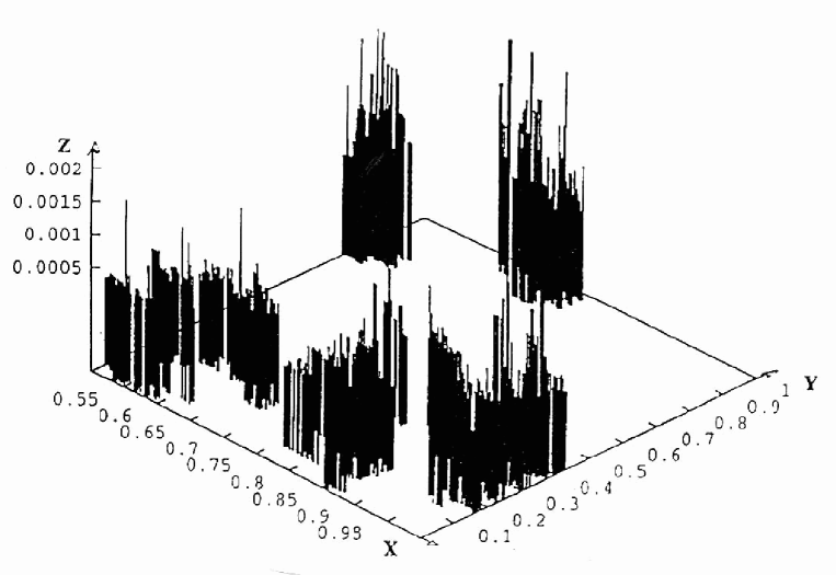
Figure 105: A random multifractal obtained by the $random-\beta-model$ algorithm in the two dimensional Euclidean space.

(1) The two point number-number correlation function

We have seen that the characteristics of a MF distribution is the $f(\alpha)$ spectrum of exponents. The relation of the properties of this distribution with the usual correlations analysis is straightforward. The exponent that describes the power law behavior of the number density corresponds to the support of the MF distribution and therefore it is related to the maximum of $f(\alpha)$ (see Sec.5.1).

(2) Luminosity function

The function $N(\mu)$ (Eq.165) for the random $\beta$ model of Fig.105 can be fitted by a power law with $\delta=-1$ and with an exponential cut-off [47]. Consider a portion of a MF distribution in a spherical volume of radius $R$. The number of singularities of type $\alpha$ in the range $[\alpha,\alpha+d\alpha]$, is given by Eq.161. The corresponding average space density scales therefore as $<\nu(\alpha,R)>\sim R^{(f(\alpha)-3)}$. This relation implies that the space density is a complex function of $\alpha$ and $R$. Although not strictly valid, a separation between a space and a luminosity distribution is useful in the analysis of real catalogs. We approximate such a separation as follows. Integrating Eq.161 in $d\alpha$ we obtain that the total number of boxes of size $\epsilon$, divided for the volume, is

$$n(R)=\frac{N(\epsilon(R))}{V}=\frac{3}{4\pi}BR^{D(0)-3}$$ (172)

where the last equality follows from the mass-length relation.

The probability that a certain box (at a given scale $\epsilon$) has the measure in the range ($\mu$, $\mu+d\mu$) is determined by Eq.165 (or Eq.169). Hence the average number of boxes for unit measure and unit volume can be written as

$$<\nu(R,\mu)>=\frac{3}{4\pi}BR^{D(0)-3}\mu^{\delta}e^{-\frac{\mu}{\mu^{*}}}$$ (173)

This equation can be read as the average probability of having a galaxy of a certain luminosity and in a certain volume, in a MF Universe.

The amplitude of $\nu(R,\mu)$ is related to the lower cut-offs of the distribution and of the sample size, and therefore has no special physical meaning. We stress in what follows (see (5)) that the shape of the LF is not completely independent on the size of the sample volume. This implies that the approximation of Eq.173 does not strictly hold, because it does not consider the correlation between space and luminosity distribution, which for MF we know to be an important feature (see (6)). Nevertheless we stress that Eq.173 can be used in practice in the analysis of real redshift surveys, with great accuracy. In fact, the result of Eq.173 has been obtained under the approximation of Eq.171, while in the more general case the cut-off $\mu^{*}$ depends explicitly on the sample size. However such a behavior is very weak in the available samples.

In summary, in order to study a MF distribution the three dimensional volume must be well defined: only in such a kind of volume one may define the scaling properties of the MF. This implies that an understanding of the distortions of the LF shape requires that volume limited samples should be used, rather than magnitude limited ones. Several authors, by analyzing the mean density in redshift surveys (i.e. the amplitude of the LF), concluded that the samples are not large enough to be fair because the fluctuations are too large [37] [184]. Our conclusion is that in magnitude limited samples it is still possible to use the inhomogeneity-independent technique to determine, if the galaxy distribution is MF, the shape of the LF, but its is certainly not possible to recover the amplitude of the LF, which is related to the space distribution via the average density. To this end one should consider a volume limited sample and normalize for the global luminosity selection which is related to such a sample (see Sec.3).

(3) Morphological and luminosities properties: a new interpretation of ”luminosity segregation”

Massive galaxies are mostly found in rich clusters while field galaxies are usually spirals or gas rich dwarfs (see Sec.2). These observational properties are consistent with multifractality, i.e. with the self-similar behavior of the whole matter distribution (Fig.105). The largest peaks are located in the largest clusters. For the self-similarity each point of the structure belongs to a cluster or to a group of galaxies, because a certain portion of the fractal distribution is always made of smaller and smaller structures. Moreover the observations that the dwarf and low-surface-brightness galaxies do not fill the voids, is consistent with the fact that the galaxy distribution continues to be fractal even for the lowest peaks of the MF. In this picture the giant-to-dwarf ratio depends on the environmental density. In fact, the dwarf galaxies can belong to the rich clusters where the giants lie, but they can also be in small groups. The morphological-segregation can be seen as the self-similar character of the matter distribution. Multifractality is a description that can be useful for the statistical characterization of the system, but, of course, it cannot explain various evidences which require a more appropriate morphological analysis.

From our result we can conclude that the fractal nature of galaxy distribution in the available samples, can account for the scaling of $r_{0}$ with sample depth. In this sense the luminosity segregation, intended as a different clustering properties of brighter and fainter galaxies in terms of the amplitude of the standard correlation function (see Sec.3 and Sec.4) has no experimental support. The linear dependence of $r_{0}$ on the sample size can be completely explained by the fractal nature of galaxy distribution. The correct perspective to describe the different clustering of brighter and fainter galaxies is the MF picture, for which we have given ample evidences, and which implies that massive are mostly into large clusters as observed. The quantitative characterization of such a phenomenon is therefore in terms of the exponent of the correlation function rather than its amplitude. In particular the brighter galaxies should have a greater correlation exponent than the fainter ones (see (4)).

(4) Multifractal spectrum and Multiscaling

Previously we have introduced the MF spectrum $f(\alpha)$ and now we clarify its basic properties. Multifractality implies that if we select only the largest peaks in the measure distribution, the set defined by these peaks may have different fractal dimension than the set defined by the entire distribution. One can define a cut-off in the measure and consider only those singularities which are above it. If the distribution is MF the fractal dimension decreases as the cut-off increases. We note that, strictly speaking, the presence of the cut-off can lead (for a certain well defined value of the cut-off itself) to the so-called multiscaling behavior of the MF measure [188]. In fact, the presence of a lower cut-off in the calculation of the generalized correlation function affects the single-scaling regime of $\chi(\epsilon,q)$ for a well determined value of the cut-off $\alpha_{cut-off}$ such that $\alpha_{cut-off}<\alpha_{c}$, and this function exhibits a slowing varying exponent proportional to the logarithm of the scale $\epsilon$. However some authors [189] misinterpret the multiscaling of a MF distribution as the variation of the fractal dimension with the density of the sample. The fractal dimension $D$ of the support corresponds to the peak of the $f(\alpha)$-spectrum and raising the cut-off implies a drift of $\alpha$ towards $\alpha_{min}$ so that $f(\alpha)<D$. This behavior can be connected with the different correlation exponent found by the angular correlation function for the elliptical, lenticular and spiral galaxies.

In particular the observational evidence is that the correlation exponent is higher for elliptical than for spiral galaxies: this trend is compatible with a lower fractal dimension for the more massive galaxies than for the smaller ones, in agreement with a MF behavior.

(5) Scaling of the maximum mass

As shown in [2] an important feature of the $f(\alpha)$ spectrum is represented by the value at $\alpha_{min}$: $f(\alpha_{min})$. This exponent corresponds to the scaling of the maximum singularity

$$\mu_{max}(\varepsilon)\sim\varepsilon^{\alpha_{min}}$$ (174)

where $\mu_{max}(\varepsilon)$ id the maximum measure among all the boxes corresponding to a gridding of size $\varepsilon$. The corresponding maximum density $\rho_{max}$ is therefore $\rho_{max}\sim\mu_{max}/\varepsilon^{3}$ where $\varepsilon\sim 1/R_{s}$ and $R_{s}$ is the total size of the system. Under the physical assumption that the maximum mass $M_{max}$ is related to the maximum density one can conclude that:

$$M_{max}\sim R_{s}^{3-\alpha_{min}}$$ (175)

i.e. that the maximum galaxy mass we can observe in a certain sample is related to the size of the sample itself. To study such an effect the sample size should be varied over a large range of length scales. In practice the depth of the VL samples which can be extracted from the available redshift surveys does not allow one to detect the scaling implied by Eq.175 so that the inhomogeneity-independent method in magnitude limited samples remains the most suitable to study the shape of the LF.

(6) Correlation between space and luminosity distribution

In [51] we have performed a test to check the MF nature of the observed Perseus-Pisces catalog. We have randomized the absolute magnitudes of the galaxies, i.e. we have fixed the galaxy position and we have assigned to each galaxy an absolute magnitude chosen at random among all the other galaxies. By doing this one destroys the correlations between the spatial locations and magnitudes of galaxies. As shown in Fig.104, in this case the behavior of $\>\tau(q)$ versus $\>q$ is linear, as for a simple fractal, with slope $\approx 2$. Instead in Fig.105 we show that the original distribution as a curved shape for $\tau(q)$. This result shows that the locations of galaxies are intrinsically correlated with their luminosities, i.e. there exists a luminosity-position correlation. The MF framework provides a mathematical tool to study such a correlation.

8.6 Theoretical implications

In this section we have shown that it is possible to frame the main properties of the galaxy space and luminosity distribution in a unified scheme, by using the concept of multifractality (MF). In fact, the continuous set of exponents $[\alpha,f(\alpha)]$ which describes a MF distribution can characterize completely the galaxy distribution when one considers the mass (or luminosity) of galaxies in the analysis. In this way many observational evidences are linked together and arise naturally from the self-similar properties of the distribution. Considering a MF distribution, the usual power-law space correlation properties correspond just to a single exponent of the $f(\alpha)$ spectrum: such an exponent simply describes the space distribution of the support of the MF measure. Furthermore the shape of the luminosity function (LF), i.e. the probability of finding a galaxy of a certain luminosity per unit volume, is related to the $f(\alpha)$ spectrum of exponents of the MF. We have shown that, under MF conditions, the LF is well approximated by a power law function with an exponential tail. Such a function corresponds to the Schecther LF observed in real galaxy catalogs. In this case the shape of the LF is almost independent on the sample size. Indeed we have shown that a weak dependence on sample size is still present because the cut-off of the Schecther function for a MF distribution turns out to be related to the sample depth: $L^{*}$ increases with sample depth. In practice as this quantity is a strongly fluctuating one, in order to study its dependence on the sample size one should have a very large sample and should vary the depth over a large range of length scales. Given this situation a sample size independent shape of the LF can be well defined using the inhomogeneity-independent method in magnitude limited samples. Indeed such a technique has been introduced to take into account the highly irregular nature of the large scale galaxy distribution. For example a fractal distribution is non-analytic in each point and it is not possible to define a meaningful average density. This is because the intrinsic fluctuations which characterize such a distribution can be large as the sample itself, and the extent of the largest structures is limited only by the boundaries of the available catalogs. Moreover if the distribution is MF, the amplitude of the LF depends on the sample size as a power law function. To determine the amplitude of the LF, as well as the average density, one should have a well defined volume limited sample, extracted from a three dimensional survey (Sec.3).

These results have important consequences from a theoretical point of view. In fact, when one deals with self-similar structures the relevant physical phenomenon which leads to the scale-invariant structures is characterized by the exponent and not the amplitude of the physical quantities which characterizes such distributions.

Indeed, the only relevant and meaningful quantity is the exponent of the power law correlation function (or of the space density), while the amplitude of the correlation function, or of the space density and of the LF, is just related to the sample size and to the lower cut-offs of the distribution. The geometric self-similarity has deep implications for the non-analyticity of these structures. In fact, analyticity or regularity would imply that at some small scale the profile becomes smooth and one can define a unique tangent. Clearly this is impossible in a self-similar structure because at any small scale a new structure appears and the distribution is never smooth. Self-similar structures are therefore intrinsically irregular at all scales and correspondingly one has to change the theoretical framework into one which is capable of dealing with non-analytical fluctuations. This means going from differential equations to something like the Renormalization Group to study the exponents. For example the so-called ”Biased theory of galaxy formation” [190] is implemented considering the evolution of density fluctuations within an analytic Gaussian framework, while the non-analyticity of fractal fluctuations implies a breakdown of the central limit theorem which is the cornerstone of Gaussian processes [1, 2, 15, 9].

In this scheme the space correlations and the luminosity function are then two aspects of the same phenomenon, the MF distribution of visible matter. The more complete and direct way to study such a distribution, and hence at the same time the space and the luminosity properties, is represented by the computation of the MF spectrum of exponents. This is the natural objective of theoretical investigation in order to explain the formation and the distribution of galactic structures. In fact, from a theoretical point of view one would like to identify the dynamical processes which can lead to such a MF distribution.

As a preliminary step in this direction we have developed a simple stochastic model [192, 193] in order to study which are the fundamental physical effects which lead to such a MF structure in an aggregation process. This is a very complex problem but to study it correctly one has to use the appropriate concepts and statistical tools. If a crossover towards homogeneity would eventually be detected, this would not change the above discussion but simply introduce a crossover into it. The (multi)fractal nature of the observed structures would in any case, require a change of theoretical perspective.

9 Conclusions and theoretical implications

Cosmology, as a part of Physics, is an experimental science and, for this reason, all the assumptions and the relations of the various models must have a solid empirical basis. Since twenty years, there has been a very fast development of the experimental techniques in this field. For example in 1980 only one thousand redshifts of galaxies were known, while now there are available about 100 thousand and in five year the number of redshifts will be more than one million. The possibility of studying the large scale structure of the Universe in various electromagnetic bands (from the radio and microwaves to the $\gamma$ and X rays) with satellite instruments, improved dramatically our knowledge of the Universe. However, despite this great observational effort, the most popular theoretical models, and in particular the Hot Big Bang theory and related galaxy formation models, encounter strong difficulties and new observations requires new ”ad hoc” explanations and, often, the introduction of new free parameters.

From an experimental point of view, there are four main facts in cosmology which are [9]: i) the space distribution of galaxies and clusters, ii) the cosmic microwave background radiation (CMBR), iii) the linearity of the redshift-distance relation, usually known as the Hubble law, iv) the abundance of light elements.

The theoretical problem is to explain these four independent experimental evidences through an unique and self-consistent picture. The current idea of standard Cosmology [4, 3] is that in the observable Large Scale Structure distribution, isotropy and homogeneity do not apply to the Universe , but only to a ”smeared-out ” Universe averaged over regions of order $\>\lambda_{0}$. One of the main problems of observational cosmology is, therefore, the identification of $\>\lambda_{0}$, The standard model assumes the homogeneity of matter distribution and deduces, from the solution of Einstein’s field equations, the linearity of Hubble law. Moreover, in the Hot Big Bang scenario, the CMBR is explained as the relict of a primordial epoch, when the matter and radiation were in thermodynamical equilibrium. The lack of an observational evidence in favor of homogeneity is therefore a crucial point for the standard Big Bang scenario. We briefly review in what follows the main theoretical implications of our results.

9.1 Cosmological Principle

The main cosmological theories are based on the assumption of the homogeneity of matter distribution. The reason is essentially the following. The basic hypothesis of a post-Copernican Cosmological theory is that all the points of the Universe have to be essentially equivalent: this hypothesis is required in order to avoid any privileged observer. This assumption has been implemented by Einstein in the so-called Cosmological Principles (CP): all the positions in the Universe have to be essentially equivalent, so that the Universe is homogeneous. This situation implies also the condition of spherical symmetry about every point, so that the Universe is also Isotropic. There is a hidden assumption in the formulation of the CP with regard to the hypothesis that all the points are equivalent. Namely, the condition that all the occupied points are statistically equivalent with respect to their environment corresponds to the property of Local Isotropy. It is generally believed that the Universe cannot be isotropic about every point without being also homogeneous [4]. Actually, Local Isotropy does not necessarily implies homogeneity; in fact a topology theorem states that homogeneity is implied by the condition of local isotropy together with the assumption of the analyticity or regularity for the distribution of matter. A fractal distribution, being locally isotropic around each point of the distribution, is perfectly compatible with a weaker version of the CP [14, 2, 16]. In addition this also implies that the tests of dipole moment saturation are only tests of local isotropy, but not homogeneity. We have shown in fact that the dipole moment tends to saturate also in a fractal structure, depending on the morphological features of the distribution, while the monopole moment grows as the power law of the sample size [16]. This is an important property of stochastic fractal structures which plays an important role in the interpretation of the large scale peculiar velocities.

9.2 The Hubble - de Vaucouleurs Paradox

The basic assumption of the Big Bang is the hypothesis that the universe is spatially homogeneous and isotropic [4]. Homogeneity of matter distribution plays the central role in the standard expanding universe model, because homogeneity implies that the recession velocity is proportional to distance [4, 3]. This means that linear velocity-distance law $v_{exp}=Hl$ is valid at such distance scales where matter distribution can be considered on average as uniform.

For a long time it was believed the deflections from homogeneity occur only inside ”inhomogeneity cells” with size (about 5-10 Mpc) corresponding to a few average distances between galaxies. Hence the homogeneity of the universe can be understood in the same sense as that of a fluid or gas, i.e. as a ”smeared-out” universe averaged over cells of inhomogeneity. Expansion of such a cosmological fluid naturally obeys the linear velocity-distance relation.

From our results (see Sec.6 for a summary) the size of the inhomogeneity cell has increased upwards to at least 150 $h^{-1}Mpc$ or more. Thus in the context of the standard model, one would expect strong deflections from the linearity of the redshift-distance relation deep inside inhomogeneities [207, 208] while observations show an almost strictly linear Hubble law starting immediately beyond the Local Galaxy Group [194]. We have explored the apparent contradiction between the linearity of the Hubble law and the inhomogeneity of galaxy distribution and discuss its implications for Cosmology in various papers [9, 195] and here we briefly review our main results.

9.2.1 Standard Model and the linear velocity-distance law

According to the Standard Model the universe is homogeneous, isotropic and expanding [4, 3]. Homogeneity of matter distribution is the heart of the standard Cosmology because it allows one to introduce the space of uniform curvature in the form of the Robertson-Walker (RW) line element. This line element leads immediately to the strict linear velocity-distance law [196, 197]. Indeed, the proper distance $l$, at cosmic time $t$, of a comoving body with fixed coordinate from a comoving observer is $l=R(t)r$. So the expansion velocity $v_{exp}=dl/dt$ defined as the rate of change of the proper distance $l$ is

$$v_{exp}=Hl=c\cdot l/l_{H}$$ (176)

where $H=\dot{R}/R$ is the Hubble constant, $l_{H}=c/H$ is the Hubble distance. In this way, the linear velocity-distance relation of Eq.176 is a rigorous consequence of spatial homogeneity and valid for all distances $l$. In particular, for $l>l_{H}$, the expansion velocity $v_{exp}>c$. Such an expanding and curved space is consistent with special relativity locally and general relativity globally [196].

In the expanding space the wavelength of an emitted photon is progressively stretched, so that the observed redshift $z$ is given by Lemaitre’s redshift law

$$z=R(t_{obs})/R(t_{em})-1$$ (177)

which is a consequence of the radial null-geodesic of the RW-line element. For $z\ll 1$ (Eq.177) yields $z\approx dR/R\approx H_{0}dt\approx l/l_{H}$, and from Eq.176 one gets the approximate velocity-redshift relation which is valid for small redshifts

$$v_{exp}\approx cz$$ (178)

It is important to emphasized that the expansion velocity-redshift relation differs from the relativistic Doppler effect. So, the space expansion redshift mechanism in the standard model is quite distinct from the usual Doppler mechanism. We stress this, because homogeneity alone does not tell which is the cause of the redshift.

9.2.2 Observed Hubble Law

In the famous paper [198] Hubble found a roughly linear relation between spectral line displacement $z=(\lambda_{obs}-\lambda_{em})/\lambda_{em}$, expressed according to the spectroscopic tradition as radial velocity $cz$, and distance $d$, which can be written as:

$$cz=H_{0}d$$ (179)

Hubble’s ’radial velocity’ was a technical term which did not refer to any interpretation of redshift, though he had in mind especially the de Sitter effect [199]. Space expansion, Doppler mechanism, and de Sitter effect yield at first order Eq.179. Hence in case of motion

$$V\approx H_{0}d$$ (180)

where $V$ is either space expansion velocity $v_{exp}$ or usual velocity, and $d$ is the distance measured by astronomer. It has been natural to interpret this law as reflecting Eq.176 and Eq.178 in the context of the standard Cosmology, and to regard the coefficient of proportionality $H_{0}$ in Eq.179 as the present value of the theoretical Hubble constant $H$ from Eq.176.

Since its discovery, the validity of the Hubble law has been confirmed within an ever increasing distance interval where local and more distant distance indicators may be tied together. Recently, several new Cepheid distances have been measured to local galaxies, thanks to the HST programs [215, 216]. Along with previous Earth-based Cepheid distances, methods like Supernovae Ia and Tully-Fisher have been better calibrated than before [216], and confirm the linearity with good accuracy up to $z\approx 0.1$ [194]. Brightest cluster galaxies trace the Hubble law even deeper, up to $z\approx 1$, and radio galaxies have provided such evidence at still larger redshifts [194].

It is well known that there are small deviations $\delta V$ from the Hubble law, connected with local mass concentrations such as the Virgo Cluster, and, possibly the Great Attractor.

However, these perturbations are still only of the order $\delta V/V_{H}\sim 0.1$, while in the general field the Hubble law has been suggested to be quite smooth, with $\delta V$ around $50km/s$ [194].

There have been proponents of global non-linearity of the Hubble law [7, 200]. However, it has been convincingly shown that such deviations from linearity are easily produced by the Malmquist bias in magnitude limited samples [201, 202, 194] and when one by-passes this problem using suitable methods, the linearity is recovered. The second main advancement is concerned with measurement of the value of the Hubble constant $H_{0}$. Since Hubble’s $559km/s/Mpc$, $H_{0}$ has decreased and according to the most recent studies [216] utilizing the increased set of Cepheid-calibrators, seems to be stabilized at about $55km/s/Mpc$.

9.2.3 The Paradox

The Hubble and de Vaucouleurs laws describe very different aspects of the Universe, but both have in common universality and observer independence. This makes them fundamental cosmological laws. Hence, it is important to compare the range of distance scales where they exist. In Fig.106 we display these laws together.

Figure 106: Hubble redshift-distance and de Vaucouleurs density-distance laws in the distance scales from $1$ to $500Mpc$ ($H_{0}=55km/s/Mpc$). The Hubble law (increasing from left to right) is constructed from: galaxies with Cepheid-distances for $cz>0$ (triangles), galaxies with Tully-Fisher (B-magnitude) distances (stars), galaxies with SNIa-distances for $cz>3000km/s$ (filled circles). TF-distance points are generally averages of a few tens of galaxies from the ”unbiased plateau” of the method of normalized distances. Redshift $cz$ is reduced to the Local Group center and contains the small correction due to the Virgo infall velocity field. The solid line corresponds to the Hubble law with $H_{o}=55km/s/Mpc$. The de Vaucouleurs law (decreasing from left to right) in the normalized form is constructed from the computation of the conditional average density. The dotted line corresponds to the de Vaucouleurs law with correlation exponent $\gamma=1$, i.e. $D=2$.

The puzzling conclusion from Fig.106 is that the strictly linear redshift-distance relation is observed deep inside the fractal structure. This empirical fact presents a profound challenge to the standard model where the homogeneity was the basic explanation of the Hubble law, and ”the connection between homogeneity and Hubble’s law was the first success of the expanding world model” [197]. This also reminds of the natural reaction ”In fact, we would not expect any neat relation of proportionality between velocity and distance [for such close galaxies] [203]. However, contrary to the expectations, modern data show a good linear Hubble law even for nearby galaxies.

9.2.4 Implications

We discuss shortly the cosmological significance of the HdeV diagram, using a minimum of assumptions. Especially, we illustrate its importance by discussing two opposite possibilities, depending on which is more fundamental law in Fig.106. There may be a homogeneously distributed dark matter, producing the linear Hubble law, while the fractal structure is just confined to the less important luminous matter. Or, the Universe may be dominated, in terms of mass, by the fractal structure, observed for the visible matter.

Alternative I: Homogeneous dark matter

The observed scale-invariant density-distance law is related to the luminous matter, i.e. the stars of the galaxies. Because the fractal distribution is inhomogeneous at all scales, this implies within the standard model that there must be something other than visible galaxies which is uniformly distributed in the universe. This could well be a homogeneous substratum of dark matter. Of course, this is not the first time when a dark mass component is proposed from other considerations, however we emphasize the simple argument following from Fig.106.

Assume that the Universe contains a large amount of its mass in the form of some unknown dark matter which has always filled the space uniformly and carried at rest in the comoving system the primordial seed density fluctuations around which later were to form the luminous galaxies. Then only at scales where the homogeneous dark mass density presently dominates over the luminous, inhomogeneous mass, the linear Hubble law can be observed. In other words, only in scales where the matter distribution looks homogeneous, one can speak about the Hubble law. This simple argument is quite strong: a dark matter component coupled to galaxies is not sufficient. One needs a truly homogeneous substratum, both at small scales in view of the good Hubble law, and at very large scale where one already starts approaching the Hubble length scale.

The argument about the required dominance of the homogeneous substratum can be made more quantitative within the linear perturbation theory which predicts that in the scale where the Hubble velocity is $V_{H}$ and density perturbation is $\delta\rho$, the peculiar velocity $\delta V$ has attained a value

$$\delta V/V_{H}=\Omega^{0.6}\delta\rho/\rho_{0}$$ (181)

where $\rho_{0}$ is the mean cosmological density. E.g., for $\Omega=1$, it is clear that small $\delta V/V_{H}$ (good Hubble law) needs small $\delta\rho/\rho_{0}$. Because at small scales the fluctuations of the inhomogeneous galaxy distribution are comparable to the average density $<\rho_{gal}>$, the uniform dark mater substance must have density high enough and fluctuations small enough in order to reduce $\delta\rho/\rho_{0}$ to its small value suggested by $\delta V/V_{H}$. This means in practice that the dark matter density must not be less than the galaxy density in the scale concerned.

With $\Omega<1$ the mean density is less than the critical one, which more than compensates the influence of the factor $\Omega^{0.6}$ in Eq.181 ($\delta\rho$ coming from galaxy distribution remains the same), and the above argument is still valid.

How smooth is this dark substratum and what is its density, or at what minimum scales it may be regarded as homogeneous and dominant?

Because the Hubble law (in Fig.106) for the field galaxies around the Local Group (LG) starts around $1\div 2Mpc$, this gives the scale where the dark substratum is already close to homogeneous and dominant. Also the detailed analysis of the velocity field of the LG galaxies in [204] showed the existence of the expansion down to $\sim 1.5Mpc$ from the LG. Additional, quite strong evidence for such a small size of the scale where the Hubble law still exists, is given by the very small internal dispersion ($\sigma<60$km/s) inferred from the Hubble diagram in the local velocity field [194]. The scale should be less than $\sigma/H_{o}$, as one may see by considering the line of sight traversing cells where the Hubble law collapses.

In order to estimate the required minimal density of the uniform dark matter, we use two estimates of the mass tied to LG galaxies. From the rotation curves the masses of the Galaxy and M31 yield [205] the sum $\approx 6.3\cdot 10^{11}M_{\bigodot}$. If one smooths out this mass in the volume $4\pi/3(1.5Mpc)^{3}$ one finds an average density $\rho(r)\approx 0.4\cdot 10^{-29}gcm^{-3}$. This value should be exceeded by the density of the uniform dark matter. As the critical density for the standard model is $\rho_{crit}=1.9\cdot 10^{-29}h^{2}gcm^{-3}$, this means that the density parameter for dark matter $\Omega_{dark}>0.6$ for $h=0.55$. The second mass estimate comes from dynamical studies of the LG yielding [204, 206] the combined mass $\approx 3\cdot 10^{12}M_{\bigodot}$. Similarly, this gives $\Omega_{dark}>3$.

The first lower limit $\Omega_{dark}>0.6$ is interestingly close to the critical value $\Omega=1$. The dynamical limit $\Omega_{dark}>3$ seems to contradict the available data for the classical cosmological tests [194].

Alternative II: Matter is tied to galaxies

(a) Spherical symmetric inhomogeneities

Instead of looking at the HdeV paradox with the aid of the dark substratum, one may choose to investigate the implications of inhomogeneous cosmologies. Spherical symmetrical inhomogeneity has been used [207, 208] to represent isotropic fractal, with the conclusion that there is a strong deflection from linear Hubble law inside a fractal inhomogeneity cell. The Lemaitre-Tolman-Bondi (LTB) solution of Einstein equations was utilized [209] for modeling a relativistic fractal Cosmology, and it was concluded that it is difficult to get a linear redshift-distance law.

We stress that, in order to be solvable, these models introduce one or more privileged points that are the center of the LTB metric. This breaks the symmetry of the problem and one models the fractal structure with an analytical density behavior. In these models the Hubble law is just an accident: this probably occurs because the isotropy of the distribution is broken rather than because a fractal is really incompatible with linearity of Hubble law. In fact, one may conjecture that the Hubble law is a consequence of isotropy rather than of homogeneity. Clearly this situation (non analytical matter distribution) has never been studied and it requires very complex models to be analyzed.

To save the linearity of the redshift-distance relation it was suggested [210] that our Galaxy is situated in a large void. However, this would put us in a privileged position, while a typical place of a galaxy, belonging to the fractal structure, is within a fractal cluster [16]. So, in the light of the LTB model the Hubble law is an accidental or luckily observed phenomenon of the universe.

(b) Fractal universe and cosmological gravitational redshift

One should not ignore the alternative possibility that the de Vaucouleurs law could be fundamental for Cosmology [7]. Similarly as the Cosmological Principle of homogeneity predicts Hubble law in the standard model, it is tempting to ask whether the more general fractal distribution can predict Hubble law in some other context.

Even though such a Cosmology has not been yet developed, one can safely say that a Hubble law due to expansion is not expected, because of the global non-uniformity. If the linear Hubble law is, however, observed, its origin must be dominated by something other than expansion.

The only known mechanism, other than Doppler effect and space expansion, to produce redshift is gravitational effect. Bondi [211] demonstrated that cosmological redshift is due to two causes: relative motion and gravitation effect. The spectral shift depends on the relative motion of source and observer, and also on the global matter distribution. In fact, it was proposed [212] that within a static homogeneous Einstein model there is the gravitational redshift $z$ which is proportional to the square of the distance.

It should be emphasized that the gravitational part of the cosmological spectral shift is redshift [211, 212] and not blueshift, as it has been supposed [213]. This choice follows from a causality argument: the emission of a photon precedes its absorption by observer’s light detector. It is also a strict consequence of the general Mattig’s relation between proper distance and redshift [9].

It has been pointed out [214] that while in the homogeneous case the gravitational redshift increases as the square of distance, inside a hierarchical structure with correlation exponent $\gamma=1$, the redshift is linearly proportional to distance, producing the Hubble $(z-d)$ relation. Indeed, if $\rho(d)\sim 1/d$, then mass $M\sim d^{2}$, and gravitational potential $\phi\sim M/d\sim d$. So the gravitational redshift $z\sim\phi/c^{2}\sim d$. In this case the value of the Hubble constant is determined by

$$H_{grav}=2\pi G\rho_{0}d_{0}/c$$ (182)

where $\rho_{0}$ and $d_{0}$ are the density and radius of the lower cut-off in the fractal structure, $G$ is the gravitational constant. If the product $\rho_{0}d_{0}=1/2\pi gcm^{-2}$ is valid in the fractal universe, then $H_{grav}=G/c=69km/s/Mpc$. It is an interesting fact that for an average galaxy with $\rho_{0}=5\cdot 10^{-24}gcm^{-3}$ and $d_{0}=10kpc$ this condition is fulfilled. Naturally, this explanation of the paradox is based on a non-standard approach to the cosmological redshift [9].

9.3 The Cosmic Microwave Background Radiation

The best known background radiation is the Cosmic Microwave Background Radiation (CMBR) [217]. After Relict and COBE experiments, the CMBR anisotropies and spectrum are well known [218, 219, 220, 221]. The perfect thermal Planck spectrum of the CMBR and its very small anisotropies are among the most important observational cosmological facts.

Few groups have detected CMBR anisotropies at various angular scales, while many other have obtained upper limits only. The amplitude of these fluctuations, after having taken into account the various spurious contributions, is of the order of some $\>\Delta T/T\sim 10^{-5}$. However it is very hard to decide if the signals observed by Relict 1 [222], by COBE [223] and other groups, are CMBR anisotropies or a mixture of CMBR and spurious signals. These results pose some trouble for the Standard Model. In fact, in the standard scenario of galaxy formation, small amplitude primordial perturbations to the energy density are amplified by gravitational instability as the Universe expands and they are predicted to leave a detectable imprint on the CMBR. Such low amplitude measured fluctuations are not compatible with the standard baryonic matter and hence in many theories of galaxy formation one must introduce some exotic kind of non baryonic matter, that has a weaker interaction with photons than the baryonic one. Such non baryonic dark matter should contribute to the density of the universe, with more than $95\%$ of the total density. Moreover, on large angular scales (few degrees), the dominant mechanism by which density fluctuations induce anisotropy in the CMBR is the Sachs-Wolf effect [224]. This is a gravitational effect due to the presence of matter between the CMBR and the observer. For this reason, the existence of large-scale structures can represent a serious problem due to their incompatibility (in the standard scenario) with such low amplitude temperature fluctuations [9].

An important point in this discussion is represented by the isotropic nature of fractal structures and in particular it is important to notice that the presence of highly isotropic distribution of objects as optical galaxies, radio-galaxies, and so on is compatible with an inhomogeneous and scale invariant distribution in the three dimensional space. However a complete discussion of the CMBR goes beyond the scope of this review.

9.4 Galaxy bulk flows

An important kind of large-scale measurement of motions is the so-called ”bulk” flow which is the estimate of the net velocity $\><V>$ of galaxies within a large volume. There are evidences [225] of large-scale coherent flows, and a coherent motion on very large volume ($\>\sim 150h^{-1}Mpc$) has been found, that implies an increase of $\><V>$ on scales much larger than that of the GA. If the CMBR dipole is due to Doppler effect then the Local Group (LG) has a velocity of $\>620kmsec^{-1}$ with respect to the rest frame represented by the CMBR. The origin of this motion can be due to some anisotropic mass fluctuation whose amplitude is expected (in an homogeneous picture) to decrease with increasing scale. Hence the bulk flows of galaxies contained in very large volume should be at rest with respect to the CMBR. The results of Lauer & Postman [226] show, on the contrary, that the LG motion relative to an Abell clusters sample is inconsistent with the velocity of the LG inferred form the CMBR dipole, and imply that the CMBR dipole anisotropy is generated by a very large scale mass concentration beyond $\>100h^{-1}Mpc$. Moreover Mathewson et al.[227] found that there is not backside infall into the GA and that there is evidence of a bulk flow of $\>600kmsec^{-1}$ in the direction of the GA on a scale at least $\>60h^{-1}Mpc$. Recently Mathewson & Ford [228] found that the flow is not uniform over the GA region and that it seems to be associated with a denser region which participates in the flow too.

From the data now available it emerges that the full extent of the galaxies flows is still uncertain and not detected and the origin of these large amplitude and coherent length peculiar motions is very unclear in the standard scenario. In fact it is very hard to reconcile these results with an homogeneous picture, in which the bulk flows have to be small on large scales as the mass fluctuations have to be of small amplitude on the large scale. On the contrary, in a fractal distribution, which is intrinsically inhomogeneous, there are fluctuations in the distribution of mass at all scales; in this case large-scale coherent flows are limited only by the the property of local isotropy that characterized a fractal structure and implies that the dipole (the net gravitational force) saturates beyond a certain scale [16].

9.5 Discussion

In summary our main points are:

• The highly irregular galaxy distributions with large structures and voids strongly point to a new statistical approach in which the existence of a well defined average density is not assumed a priori and the possibility of non analytical properties should be addressed specifically.

• The new approach for the study of galaxy correlations in all the available catalogs shows that their properties are actually compatible with each other and they are statistically valid samples. The severe discrepancies between different catalogs which have led various authors to consider these catalogs as not fair, were due to the inappropriate methods of analysis.

• The correct two point correlation analysis shows well defined fractal correlations up to the present observational limits, from 1 to $1000h^{-1}Mpc$ with fractal dimension $D\simeq 2$. Of course the statistical quality and solidity of the results is stronger up to $100\div 200h^{-1}Mpc$ and weaker for larger scales due to the limited data. It is remarkable, however, that at these larger scales one observes exactly the continuation of the correlation properties at the small and intermediate scales.

• These new methods have been extended also to the analysis of the number counts and the angular catalogs, which are shown to be fully compatible with the direct space correlation analysis. The new analysis of the number counts suggests that fractal correlations may extend also to scales larger than $1000h^{-1}Mpc.$

• The inclusion of the galaxy luminosity (mass) leads to a distribution which is shown to have well defined multifractal properties. This leads to a new, important relation between the luminosity function and that galaxy correlations in space.

• New perspective on old arguments. On the light of these results we can now take a standard reference volume in the field (i.e. [3]) and consider the usual arguments invoked for homogeneity from a new point of view. These arguments are: (a) number counts: we have seen in Sec.7 that the small scale exponent of number counts is certainly not related to homogeneity but to small scale fluctuations. The real exponent of the number counts is instead the lower one (i.e. $\alpha\approx 0.4$) that indeed corresponds to the three dimensional (i.e fractal with $D\simeq 2$) correlation properties. (b) $\delta N/N$ is small for various observations. This point is exactly the same as the fact $r_{0}$ is a spurious length. In the absence of a reference average one cannot talk about ”large” or ”small” amplitude of fluctuations. In addition, for any distribution, even a fractal one $\delta N/N$ is always small for sizes comparable to the total sample because the average is computed from the sample itself. (c) Angular correlations. We have seen in Sec.7 that angular correlations are ambiguous in two respects: first the angular projection of a fractal is really uniform at large angles due to projection effects, second the angular data are strongly affected by the finite size fluctuations which provide an additional artificial homogenization, as in the case of the number counts. The inclusion of these effects reconciles quite naturally the angular catalogs with the fractal properties in the three dimensional ones. (d) X-ray background. The argument that $\delta N/N$ becomes very small for the X-ray background combines the two problems discusses before: angular projections and reference average. This angular uniformity is analogues, for example, to the Lick angular sample, and certainly is not a proof of real homogeneity.

  Finally one should note that all these arguments are indirect and always require an interpretation based on some assumptions. The most direct evidence for the properties of galaxy distribution arises from the correct correlation analysis of the 3-d volume limited samples that has been the central point of our work.

9.6 Theoretical Implications

From the theoretical point of view the fact that we have a situation characterized by self-similar structures implies that we should not use concept like $\xi(r)$, $r_{0}$, $\delta N/N$ and certain properties of the power spectrum, because they are not suitable to represent the real properties of the observed structures. To this end also the N-body simulations should be considered from a new perspective. One cannot talk about ”small” or ”large” amplitudes for a self-similar structure because of the lack of a reference value like the average density. The Physics should shift from ”amplitudes” towards ”exponent” and the methods of modern statistical Physics should be adopted. This requires the development of constructive interactions between two fields.

Possible Crossover. We cannot exclude of course, that visible matter may really become homogeneous at some large scale not yet observed. Even if this would happen the best way to identify the eventual crossover is by using the methods we have described and not the usual ones. From a theoretical point of view the range of fractal fluctuations, extending at least over three decades ($1\div 1000h^{-1}Mpc$), should anyhow be addressed with the new theoretical concepts. Then one should study the (eventual) crossover to homogeneity as an additional problem. For the moment, however, no tendency to such a crossover is detectable from the experimental data and it may be reasonable to consider also more radical theoretical frameworks in which homogenization may simply not exist at any scale, at least for luminous matter.

Dark Matter. All our discussion refers to luminous matter. It would be nice if the new picture for the visible universe could reduce, to some extent, the importance of dark matter in the theoretical framework. At the moment however this is not clear. We have two possible situations: (i) if dark matter is essentially associated to luminous matter, then the use of FRW metric is not justified anymore. This does not necessarily imply that there is no expansion or no Big Bang. It implies, however, that these phenomena should be described by more complex models. (ii) If dark matter is homogeneous and luminous matter is fractal then, at large scale, dark matter dominate the gravity field and the FRW metric is again valid. The visible matter however remains self-similar and non analytical and it still requires the new theoretical methods mentioned before.

9.7 Predictions for future surveys

Table 10: The volume limited samples of various catalogs (not still published and analyzed) are characterized by the following parameters: - $R_{VL}(h^{-1}Mpc)$ is the depth of the VL sample considered with absolute magnitude limit $M_{VL}$ - $\Omega$ is the solid angle - $R_{eff}(h^{-1}Mpc)$ is the radius of the largest sphere that can be contained in the catalog volume. This gives the limit of statistical validity of the sample. - $r_{0}(h^{-1}Mpc)$ is the length at which $\xi(r)\equiv 1$. (distance are expressed in $h^{-1}Mpc$).

Sample	$\Omega$ ($sr$)	$R_{VL}$	$M_{VL}$	$R_{eff}$	$r_{0}$
CfA2	1.83	101	-19.5	22	7
CfA2	1.83	160	-20.5	36	12
SLOAN	$\pi$	400	-19	185	60
SLOAN	$\pi$	600	-20	275	90
2dF (South)	0.28	550	-19	50	15
2dF (South)	0.28	870	-20	100	30

According to the standard interpretation, the length $r_{0}\simeq 5h^{-1}Mpc$ characterizes the physical properties of galaxy distributions. Therefore deeper samples like CfA2 and SLOAN should simply reduce the error bar, which is now about considered to be $10\%$. A possible variation of $r_{0}$ with absolute magnitude, due to a luminosity bias, is considered plausible but it has never been quantified. This should be checked by varying independently absolute magnitude and depth of the volume limited samples. However, from this interpretation, the value of $r_{0}=5h^{-1}Mpc$, corresponding to a volume limited of CfA1 with $M=-19.5$, should not change when considering in CfA2 and SLOAN volume limited samples with the same solid angle $\Omega$ and the same absolute magnitude limit ($M=-19.5$).

In our interpretation, instead, $r_{0}$ is spurious, and it scales linearly with the radius $R_{s}$ of the largest sphere fully contained in the volume limited samples. Therefore we predict for the volume limited sample of CfA2 with $M=-19.5$ (with a solid angle of $\Omega=1.1\;sr$ [38]) $r_{0}\approx 7h^{-1}Mpc$ (if, in the final version of the survey the solid angle is $\Omega=1.8$, the value of $R_{s}$ increases accordingly, and the value of $r_{0}$ is shifted up to $\sim 9h^{-1}Mpc$). Note however that for the deepest volume limited CfA2 sample ($M\mathrel{\hbox to0.0pt{\lower 3.0pt\hbox{$\mathchar 536\relax$}\hss}\raise 2.0pt\hbox{$\mathchar 316\relax$}}-20$) we predict instead $r_{0}\approx 15\div 20h^{-1}Mpc$. For the volume limited sample of the full SLOAN with $M=-19.5$ ($\Omega=\pi$), our prediction is that $r_{0}\approx 65h^{-1}Mpc$. It is clear that however, the first SLOAN slice gives smaller values because the solid angle is be small. In Tab.10 we report the predictions for $r_{0}$ in the next future surveys.

Appendixes

In the following we report the details of the various samples we have analyzed in this paper.

CfA1

The sample contains 1845 galaxies with $m_{ph}\leq 14.5$ in the northern hemisphere in a region of $1.83\;sr$ [17]. We have extracted same VL sample, and we report in Tab.11 the characteristics. The noticeably high density area in the center of the catalog is the nearby Virgo cluster.

Perseus-Pisces

The Perseus-Pisces redshift survey collects the positions and the redshifts for the galaxies in the region $22^{h}<\alpha<4^{h}$ and $\>0^{\circ}<\delta<45^{\circ}$ [40]. The survey consists mainly of highly accurate 21 cm H I line redshifts. The radio data are complemented with optical observations of early-type galaxies carried out at the 2.4 m telescope of the MacGraw-Hill Observatory, plus a number of redshifts provided by J.Huchra and other smaller sources in the public domain. The catalog used comprises those redshifts obtained before 1991 December, for a total of 5183 galaxies. Among them, 3854 have Zwicky magnitudes of 15.7 or brighter. From this sample, we have excluded the data in the region more affected by extinction; hence we have considered the data only in the ranges $[22^{h}<\alpha<3^{h}10^{m}]$ and $[0^{\circ}<\delta<42^{\circ}30^{\prime}]$, with $m\leq 15.5$.

We have studied galaxies with corrected velocity in the range $0-13,000$ $Km\dot{s}ec^{-1}$. The apparent magnitudes of galaxies have been corrected for the extinction, using the absorption maps produced by Burstein & Heiles [181]. The final sample, with apparent magnitude less than $15.5$, contains $N=3301$ galaxies (that we call hereafter PP 15.5). With these data, we have produced some VL subsamples whose characteristic are reported in Tab.12 and Tab.13

Table 11: VL samples of CfA1. Apparent magnitude limit =14.5 Total number of galaxies =1843 (cut in absolute magnitude)

Sample	$d_{lim}(h^{-1}Mpc)$	$M_{lim}$	$N$
VL18	$31.3$	$-18.00$	$480$
VL185	$39.8$	$-18.50$	$424$
VL19	$50.1$	$-19.00$	$335$
VL195	$63.1$	$-19.50$	$231$
VL20	$79.4$	$-20.00$	$200$
VL205	$100.0$	$-20.50$	$98$

Table 12: Perseus-Pisces: Apparent magnitude limit =15.5 Total number of galaxies =3301

Sample	$d_{lim}(h^{-1}Mpc)$	$M_{lim}$	$N$	$R_{s}(h^{-1}Mpc)$	$r_{0}(h^{-1}Mpc)$
VL40	$40$	$-17.53$	$291$	$8$	$3\pm 0.5$
VL50	$50$	$-18.03$	$871$	$12$	$4.5\pm 0.5$
VL60	$60$	$-18.43$	$990$	$13$	$4\pm 0.5$
VL70	$70$	$-18.77$	$975$	$16$	$5\pm 0.5$
VL80	$80$	$-19.07$	$894$	$19$	$6\pm 0.5$
VL90	$90$	$-19.33$	$780$	$20.4$	$7\pm 0.5$
VL100	$100$	$-19.57$	$688$	$23$	$7.6\pm 0.5$
VL110	$110$	$-19.79$	$451$	$24$	$8\pm 0.5$
VL120	$120$	$-19.98$	$291$	$28$	$10\pm 0.5$

Table 13: Perseus-Pisces: Apparent magnitude limit =15.5 Total number of galaxies =3301 (cut in absolute magnitude)

Sample	$d_{lim}(h^{-1}Mpc)$	$M_{lim}$	$N$
VL18	$50.1$	$-18.00$	$895$
VL185	$63.1$	$-18.50$	$1050$
VL19	$79.4$	$-19.00$	$975$
VL195	$100.0$	$-19.50$	$798$
VL20	$125.9$	$-20.00$	$468$

Then we construct some VL subsamples for the PP14.5 catalog (apparent magnitude limit $14.5$) whose characteristics are reported in Tab.14.

Table 14: Perseus-Pisces: Apparent magnitude limit =$14.5$ Total number of galaxies =$865$

Sample	$d_{lim}(h^{-1}Mpc)$	$M_{lim}$	$N$	$R_{s}(h^{-1}Mpc)$	$r_{0}(h^{-1}Mpc)$
VL40(b)	$40$	$-18.53$	$114$	$8.0$	$3.0\pm 0.5$
VL50(b)	$50$	$-19.03$	$318$	$9.0$	$3.5\pm 0.5$
VL60(b)	$60$	$-19.43$	$278$	$12.0$	$4.5\pm 0.5$
VL70(b)	$70$	$-19.78$	$205$	$15.0$	$5.0\pm 0.5$

LEDA

We refer to Sec.3.1.7 for a detailed discussion of the properties of this database, and for a list of reference where it is possible to find further informations. Here we report several tables with the characteristics of various VL samples extracted from this database.

In Tab.15 we show the characteristics of the VL samples extracted form the database limited at the apparent magnitude $14.5$ (LEDA14.5N), in the same sky region of CfA1.

Table 15: The VL subsamples of LEDA14.5N-CfA1 ($\Omega=1.8$)

SAMPLE	$d_{lim}(h^{-1}Mpc)$	$M_{lim}$	$N$	p
VL40	40	-18.54	445	8 %
VL60	60	-19.43	320	2 %
VL80	80	-20.07	226	1.1 %

In Tab.16 we show the properties of the VL samples (limited in distance) extracted from the database limited at $14.5$ (LEDA14.5N for the northern hemisphere, and LEDA14.5S for the southern one). The solid angle is $\sim 5\;sr$.

Table 16: The VL subsamples of LEDA14.5N and LEDA14.5S (North N=4703, South N=4163)

SAMPLE	$d_{lim}(h^{-1}Mpc)$	$M_{lim}$	$N$	p
VL40-N	40	-18.54	1096	8 %
VL40-S	40	-18.54	683	6 %
VL60-N	60	-19.43	838	2 %
VL60-S	60	-19.43	1088	2.3 %
VL80-N	80	-20.07	542	1.1 %
VL80-S	80	-20.07	571	1.1 %

In Tab.17 we show the properties of the VL samples (limited in absolute magnitude) extracted from the database limited at $14.5$.

Table 17: The VL subsamples of LEDA14.5N and LEDA14.5S (North N=4703, South N=4163) (cut in absolute magnitude)

Sample	$d_{lim}(h^{-1}Mpc)$	$M_{lim}$	$N$
VL18S	$31.3$	$-18.00$	$578$
VL18N	$31.3$	$-18.00$	$1138$
VL185S	$39.3$	$-18.50$	$712$
VL185N	$39.3$	$-18.50$	$1120$
VL19S	$49.3$	$-19.00$	$1034$
VL19N	$49.3$	$-19.00$	$1095$
VL195S	$61.8$	$-19.50$	$1160$
VL195N	$61.8$	$-19.50$	$844$
VL20S	$77.4$	$-20.00$	$675$
VL20N	$77.4$	$-20.00$	$634$
VL205S	$96.9$	$-20.50$	$371$
VL205N	$96.9$	$-20.50$	$282$

Tab.18 is the same of Tab.16 for the database limited at the apparent magnitude $16$ (LEDA16N and LEDA16S)

Table 18: The VL subsamples of LEDA16N and LEDA16S

SAMPLE	$d_{lim}(h^{-1}Mpc)$	$M_{lim}$	$N$	p
VL40-N	40	-17.04	2845	23 %
VL40-S	40	-17.04	1598	13 %
VL80-N	80	-18.57	4550	9 %
VL80-S	80	-18.57	4264	8 %
VL120-N	120	-19.48	3565	3 %
VL120-S	120	-19.48	3458	3 %
VL160-N	160	-20.13	1669	1 %
VL160-S	160	-20.13	1898	1 %

Tab.19 is the same of Tab.17 for the database limited at the apparent magnitude $16$ (LEDA16N and LEDA16S)

Table 19: The VL subsamples of LEDA16N and LEDA16S (North N=13362, South N=11794) (cut in absolute magnitude)

Sample	$d_{lim}(h^{-1}Mpc)$	$M_{lim}$	$N$
VL18S	$61.8$	$-18.00$	$4402$
VL18N	$61.8$	$-18.00$	$4011$
VL185S	$77.4$	$-18.50$	$4632$
VL185N	$77.4$	$-18.50$	$4827$
VL19S	$96.9$	$-19.00$	$4481$
VL19N	$96.9$	$-19.00$	$4678$
VL195S	$121.0$	$-19.50$	$3724$
VL195N	$121.0$	$-19.50$	$3761$
VL20S	$150.9$	$-20.00$	$2463$
VL20N	$150.9$	$-20.00$	$2143$
VL205S	$187.8$	$-20.50$	$1305$
VL205N	$187.8$	$-20.50$	$901$

Tab.20 is the same of Tab.16 for the database limited at the apparent magnitude $17$ (LEDA17N and LEDA17S)

Table 20: The VL subsamples of LEDA17N and LEDA17S

SAMPLE	$d_{lim}(h^{-1}Mpc)$	$M_{lim}$	$N$	p
VL40-N	40	-16.03	3766	31 %
VL40-S	40	-16.03	1975	17 %
VL120-N	120	-18.48	7388	7%
VL120-S	120	-18.48	6913	6 %
VL160-N	160	-19.13	5919	3%
VL160-S	160	-19.13	5731	3%
VL200-N	200	-19.65	3914	1.3 %
VL200-S	200	-19.65	4118	1.4 %

Tab.21 is the same of Tab.17 for the database limited at the apparent magnitude $17$ (LEDA17N and LEDA17S)

Table 21: The VL subsamples of LEDA17N and LEDA17S (North N=15407, South N=14101 (cut in absolute magnitude)

Sample	$d_{lim}(h^{-1}Mpc)$	$M_{lim}$	$N$
VL18S	$96.8$	$-18.00$	$7518$
VL18N	$96.8$	$-18.00$	$8022$
VL185S	$121.0$	$-18.50$	$7695$
VL185N	$121.0$	$-18.50$	$8083$
VL19S	$150.9$	$-19.00$	$6940$
VL19N	$150.9$	$-19.00$	$6954$
VL195S	$187.8$	$-19.50$	$5356$
VL195N	$187.8$	$-19.50$	$5002$
VL20S	$233.1$	$-20.00$	$3390$
VL20N	$233.1$	$-20.00$	$2767$
VL205S	$288.5$	$-20.50$	$1637$
VL205N	$288.5$	$-20.50$	$1187$

IRAS

The IRAS 2Jy survey (hereafter I-2) is a complete sample of galaxies uniformly selected over most of the sky. We refer the reader to Strauss et al., 1990, Strauss et al., 1992, for a detailed discussion of the sample selection. The sky coverage of the survey is $11.01sr$. The selection criteria have been chosen in relation to the infrared flux, and in particular there have been selected the galaxies with apparent flux at $60\mu m$ ($f_{60}$) greater than $1.936Jy$. This sample contains $2652$ galaxies. The IRAS 1.2 Jy survey (hereafter I-12) is a similar catalog, but it collects all the galaxies with $f_{60}>1.2Jy$, and the number of galaxies is doubled, and contains 5313 redshifts [42]. For the well-calibrated fluxes and the lack of Galactic extinction in the IRAS wavelengths, these surveys are believed to be well suited for studies of large scale distribution of galaxies.

The redshift are converted to the Local Group reference frame and no further corrections have been made for peculiar motions. In order to eliminate the possible selection effect due to the residual galactic extinction, we have separated the catalogs in two half sky samples. In this way we have for example, I-2N (I-12N) which refers to the northern hemisphere, and I-2S (I-12S) which refers to the southern one. The sample I-12N contains $N=2851$ galaxies and the sample I-12S contains $N=2480$ galaxies.

We have then built the volume limited samples (VL) from these flux limited surveys (Table 22, Table 23).

Sample (North-South)	$R_{VL}$ (Mpc)	Number	Percentage
VL40-N	40	189	1.5 %
VL40-S	40	111	0.9 %
VL60-N	60	166	0.6 %
VL60-S	60	163	0.6 %
VL80-N	80	145	0.3 %
VL80-S	80	117	0.24 %
VL100-N	100	155	0.2 %
VL100-S	100	123	0.2 %

Table 22: The VL subsamples of I-2N and I-2S

Sample (North-South)	$R_{VL}(h^{-1}Mpc)$	Number	Percentage	$\ell$
VL20-N	20	243	7.8 %	4
VL20-S	20	160	5.2 %	5
VL40-N	40	384	2.4 %	70
VL40-S	40	266	2.2 %	8
VL60-N	60	411	1.5 %	10
VL60-S	60	471	1.7 %	10
VL80-N	80	412	0.8 %	18
VL80-S	80	378	0.7 %	14
VL100-N	100	352	0.4 %	18
VL100-S	100	360	0.5 %	18
VL120-N	120	283	0.3 %	23
VL120-S	120	378	0.3 %	22

Table 23: The VL subsamples of I-12N and I-12S

Las Campanas Redshift Survey

The Las Campanas Redshift Survey contains over 26000 galaxy spectra, with an average redshift $z=0.1$, over 700 square degrees of the sky. The survey is composed by 6 slices $1.5^{\circ}$ in declination by $80^{\circ}$ in right ascension. In the North galactic hemisphere the 3 slices are centered at $\delta=-3^{\circ}\;,-6^{\circ}\;,-12^{\circ}$, while in the South hemisphere at $\delta=-39^{\circ}\;,-42^{\circ}\;,-15^{\circ}$ . The $20\%$ of the data was obtained using a 50-object fiber system, while the remaining $80\%$ of the data was taken with a 112-object system. The survey galaxies were selected in the $r-$band. For the 50-fiber data the isophotal magnitude limits are $16<m<17.3$, while for the 112-fiber data the isophotal magnitude limits are $15<m<17.7$ [41].

When there are more objects that meet the photometric criteria than fibers available in a given $1.5^{\circ}\cdot 1.5^{\circ}$ field (which composes each slice) the targets galaxies are chosen random from within the photometric boundaries. In such a way each it is possible to associate to each field a galaxy sampling fraction. The more uniform slice is the one centered at $\delta=-12^{\circ}$, and we examine this slice in what follows, by extracting some VL samples.

As the survey is limited by an upper and a lower magnitude, in order to construct VL samples, one has to put to limits in distance and absolute magnitude. We show The characteristics of the VL samples for the $\delta=-12^{\circ}$ slice in Tab.24. For example the sample SL12-2565 is limited in the distance range $250\div 650$.

Sample	$\Delta R_{VL}(h^{-1}Mpc)$	$\Delta M_{lim}$	N
SL12-2565	$250\div 650$	$-21.36\div-22.04$	507
SL12-153	$150\div 300$	$-19.68\div-20.93$	1132
SL12-125	$120\div 500$	$-19.29\div-20.05$	565
SL12-36	$300\div 600$	$-21.19\div-22.44$	651

Table 24: The VL subsamples of the LCRS (slice SL12) catalog with a double cut in distance and absolute magnitude . Total number of galaxies 5189.

ESP

This galaxy survey consists of a strip of $22^{\circ}\cdot 1^{\circ}$ plus a nearby area of $5^{\circ}\cdot 1^{\circ}$ five degrees west of the strip, in the South Galactic Pole region. The right ascension limits are $22^{h}30^{m}$ and $01^{h}20^{m}$ at mean declination $\delta=-40^{\circ}$. This area has been filed with a regular grid of circular fields with a diameter of $32\;arcminutes$ [44] (this size corresponds to the field of view of the multifiber spectrograph used). The limiting magnitude of the survey is $b_{j}\leq 19.4$. The catalog has a $95\%$ completeness at $b_{j}\leq 20.5$, a photometric accuracy of $\sim 0.03$ magnitudes and an estimated stellar contamination $\leq 10\%$. The total number of object is of the order of $4000$. The characteristics of the VL samples for the larger strip are shown in Tab.25, while in Tab.26 there are shown the numbers for the whole catalog.

Table 25: Apparent magnitude limit = 19.4 Total number of galaxies =3175 Euclidean without K-corrections.

Sample	$d_{lim}(h^{-1}Mpc)$	$M_{lim}$	$N$
ES300	$300$	$-17.98$	$641$
ES400	$400$	$-18.61$	$1006$
ES500	$500$	$-19.09$	$871$
ES600	$600$	$-19.49$	$671$
ES700	$700$	$-19.82$	$413$
ES800	$800$	$-20.11$	$204$

Table 26: Apparent magnitude limit =19.4 Total number of galaxies =2583, first region, Euclidean without K-corrections. (cut in absolute magnitude)

Sample	$d_{lim}(h^{-1}Mpc)$	$M_{lim}$	$N$
VL18	$302$	$-18.00$	$551$
VL185	$380.2$	$-18.50$	$862$
VL19	$478.6$	$-19.00$	$759$
VL195	$602.5$	$-19.50$	$508$
VL20	$758.6$	$-20.00$	$201$
VL205	$955$	$-20.50$	$32$

Stromlo-APM Redshift Survey

In this survey it has been selected galaxies randomly at the rate 1 in 20 from the complete APM magnitude limited catalog [56]. The catalog covers 4300 square degrees of the southern sky defined by $21^{h}\mathrel{\hbox to0.0pt{\lower 3.0pt\hbox{$\mathchar 536\relax$}\hss}\raise 2.0pt\hbox{$\mathchar 316\relax$}}\alpha\mathrel{\hbox to0.0pt{\lower 3.0pt\hbox{$\mathchar 536\relax$}\hss}\raise 2.0pt\hbox{$\mathchar 316\relax$}}5^{h}$ and $-72^{\circ}.5\mathrel{\hbox to0.0pt{\lower 3.0pt\hbox{$\mathchar 536\relax$}\hss}\raise 2.0pt\hbox{$\mathchar 316\relax$}}\delta\mathrel{\hbox to0.0pt{\lower 3.0pt\hbox{$\mathchar 536\relax$}\hss}\raise 2.0pt\hbox{$\mathchar 316\relax$}}-17^{\circ}.5$. The survey is essentially complete to magnitude limit of $b_{j}=17.15$ and consists of 1769 galaxies. In Tab.27 we show the characteristics of the VL samples limited in absolute magnitude. An important selection effects exists, because all the galaxies with apparent magnitudes brighter than $\sim 14.5$ are not included in the survey. In order to construct VL samples which are not biased by this effect, we have put two limits in distance, as for the case of LCRS (Tab.28, where WL12 means the VL sample limited by the distance range $100\div 200h^{-1}Mpc$).

Sample	$R_{VL}(h^{-1}Mpc)$	$M_{lim}$	N	$p$	$\ell(h^{-1}Mpc)$
VL18	107	-18.0	325	$2\%$	11
VL185	135	-18.5	406	$1.7\%$	13
VL19	170	-19.0	506	$1.3\%$	16
VL195	214	-19.5	575	1.0 %	19
VL20	269	-20.0	403	0.4 %	27
VL205	339	-20.5	176	0.1 %	44
VL21	427	-21.0	339	0.02 %	88

Table 27: The VL subsamples of the APM catalog

Sample	$\Delta R_{VL}(h^{-1}Mpc)$	$\Delta M_{lim}$	N	$p$	$\ell(h^{-1}Mpc)$
WL12	$100\div 200$	$-19.35\div-20.5$	451	1.0 %	19
WL13	$100\div 300$	$-20.5\div-20.23$	136	1.0 %	44
WL515	$50\div 150$	$-18.7\div-19.0$	104	1.0 %	23
WL1525	$150\div 250$	$-19.81\div-21.4$	367	1.0 %	24
WL23	$200\div 300$	$-20.2\div-22$	170	1.0 %	36
WL2535	$250\div 350$	$-20.6\div-22.5$	66	1.0 %	60
WL51	$50\div 100$	$-17.85\div-19.0$	170	1.0 %	13
WL115	$100\div 150$	$-18.7\div-20.5$	303	1.0 %	15
WL153	$150\div 300$	$-20.2\div-21.38$	230	1.0 %	35

Table 28: The VL subsamples of the APM catalog with a double cut in distance and absolute magnitude

SSRS1

The SSRS1 is the counterpart of the CfA1 catalog in the southern hemisphere. The selection criterion is such that this survey contains all the galaxies with $D(0)\leq 0.1$, where $D(0)$ is a ”face-on” diameter defined by [53]

$$\log D(0)=\log D_{1}-0.235A(T)\log(D_{1}/D_{2})$$ (183)

and $D_{1}$ is the major diameter, while $D_{2}$ is the minor one, $T$ is the morphological type and $A(T)=0.894$ if $T\geq 0$ or $A(T)=0.950$ for $T<0$. The northern declination boundary of the catalog is $\delta=-17^{\circ}.4$, and to avoid bias due to the absorption in the Galactic plane it has been selected galaxies below the galactic latitude $b=-30^{\circ}.0$. The sample contains 1773 objects distributed over $1.75\,sr$. In Tab.29 there are shown the characteristics of the VL samples.

Sample	$R_{VL}$ (Mpc)	$D_{lim}$	N	$p$	$\ell(h^{-1}Mpc)$
VL60	60	21.9	346	5.5 %	7
VL80	80	29.2	241	2.1 %	11
VL100	100	36.6	195	1.1 %	14
VL120	120	44	134	0.5 %	21

Table 29: The VL subsamples of the SSRS1 catalog

References

- [1] Pietronero L., Physica A, 144, (1987) 257
- [2] Coleman, P.H. & Pietronero, L., Phys.Rep. 231, (1992) 311
- [3] Peebles P. J. E., (1993) Principles of physical cosmology, Princeton Univ. Press
- [4] Weinberg S.E. (1972) Gravitation and Cosmology, Wiley & Sons, New York
- [5] Charlier C.V.L., Arkiv. for mat. Astron. Physik 4, (1908) 1
- [6] Charlier C.V.L., Arkiv. for mat. Astron. Physik 16, (1922)1
- [7] De Vaucouleurs, G., Science, 167, (1970) 1203
- [8] De Vaucouleurs, G., Publ. A.S.P. 83, (1971)113
- [9] Baryshev, Y., Sylos Labini, F., Montuori, M., Pietronero, L. Vistas in Astron. 38, (1994) 419
- [10] Klain O., Nature 211 (1966) 1338
- [11] Lerner E., IEEE Trans on Plasma Sci. PS-14 (1986) 609
- [12] Wilson K.G., Phys. Rep. 12, (1974) 75
- [13] Amit D., (1978) ”Filed Theory, the Renormalization Group and Critical Phenomena” (Mc Graw-Hill, New York)
- [14] Mandelbrot B., (1982) The Fractal Geometry of Nature, Freeman, New York
- [15] Erzan A., Pietronero L., Vespignani A., Rev. Mod. Phys. 67, (1995) 554
- [16] Sylos Labini F., Astrophys. J., 433, (1994) 464
- [17] Huchra, J., Davis, M., Latham, D., Tonry, J. Astrophys. J. .Suppl., 52, (1983) 89.
- [18] Davis, M., Peebles, P. J. E. Astrophys. J., 267, (1983) 465
- [19] Davis, M., in the Proc of the Conference ”Critical Dialogues in Cosmology” N. Turok Ed. (1997) World Scientific
- [20] Pietronero, L., Montuori, M. and Sylos Labini, F., in the Proc of the Conference ”Critical Dialogues in Cosmology” N. Turok Ed. (1997) World Scientific
- [21] Coleman, P.H. Pietronero, L.,& Sanders, R.H., Astron. Astrophys. Lett. 245, (1988), 1
- [22] Bachall N.A., & Soneira R.M., Astron. Astrophys. 270, (1983), 20
- [23] Sylos Labini F., Gabrielli A., Montuori M., Pietronero L., Physica A, 226, (1996) 195
- [24] Di Nella, H., Montuori, M., Paturel, G., Pietronero, L., Sylos Labini, F. Astron. Astrophys. Lett., 308 (1996) L33
- [25] Peebles, P.J.E. Large Scale Structure of the Universe , Princeton Univ. Press (1980)
- [26] Strauss M.A., and Willick J.A., (1995), Phys. Rep. 261, 271
- [27] Limber D.N. 1953 Astrophys.J., 117 (1953), 655
- [28] Limber D.N. 1953 Astrophys.J., 119 (1953), 655
- [29] Maddox et al., Mon.Not.R.Astr.Soc. 242, (1990) 43
- [30] Benzi, R., Paladin, G., Parisi, G., Vulpiani, A. J.Phys. A., 17, (1984) 3251.
- [31] Siebesma A.P., Ph.D. Thesis, (1989) Groningen
- [32] Mandelbrot B., Astrophys Lett & Comm (1997), in print
- [33] Falconer K, ”Fractal geometry”, J. Wiley & Sons (1990)
- [34] Montuori M. & Sylos Labini F., (1997) preprint
- [35] Grassberger, P. and Procaccia I, 1984 Physica D 13, 34
- [36] De Lapparent, V., Geller, M. J., Huchra, J. P. Astrophys. J. 332, (1988) 44
- [37] Da Costa, L. N. et al. Astrophys. J. 424, (1994) L1
- [38] Park, C., Vogeley, M.S., Geller, M., Huchra, J. Astrophys. J., 431, (1994) 569
- [39] Da Costa, L. N. et al. Astrophys. J., 327, (1988) 544
- [40] Haynes, M., Giovanelli, R., (1988) in ”Large-scale motion in the Universe”, Eds. Rubin, V.C., Coyne, G., Princeton University Press, Princeton
- [41] Schectman S. et al., Astrophys. J., (1996) 470,172
- [42] Fisher K., et al., Astrophys.J. Suppl., (1996) 100, 69
- [43] Broadhurst, T. J., et al.Nature, 343, (1990) 726
- [44] Vettolani, G., et al. (1994) Proc. of Scloss Rindberg workshop Studying the Universe with Clusters of Galaxies
- [45] Zucca E., et al. (1997) Astron. & Astrophys., in print
- [46] Peebles P.J.E., Physica D, 38, (1989) 273
- [47] Sylos Labini F. & Pietronero L., Astrophys.J., (1996), 469, 28
- [48] Schecther, P., Astrophys.J. 203, (1976) 297
- [49] Davis, M. et al. Astrophys.J.Lett., 333, (1988) L9
- [50] Vogeley M.S., Park C., Geller m.J. & Huchra J.P. Astrophys. J., 391, (1992), L5
- [51] Sylos Labini F., Montuori M., Pietronero L., Physica A, 230 (1996) 336
- [52] Guzzo L., et al Astrophys. J., 382, (1992) L5
- [53] Da Costa N., Pellegrini P., Davis M., Miksin A., Sargent W.L and Tonry J.L. Astrophys. J. Suppl., 75 (1991), 935
- [54] Maurogordato S., Schaeffer R. and Da Costa L.N., Astrophys.J. 390, (1992), 17
- [55] Benoist C., Maurogordato S., Da Costa L.N., Cappi A., and Schaeffer R., Astrophys. J., (1996), 472, 452
- [56] Loveday J., Peterson B.A., Efstathiou G. and Maddox S.J., Astrophys.J., 390 (1992), 338
- [57] Loveday J., Peterson B.A, Maddox S.J. and Efstathiou G. Astrophys.J. (1996), in press
- [58] Di Nella H., Sylos Labini F., Montuori M., Paturel G. and Pietronero L., (1996) preprint
- [59] Amendola L., Di Nella H., Montuori M., Sylos Labini F., (1997) Fractals, in print
- [60] Amendola L., Di Nella H., Montuori M., Sylos Labini F., (1997) preprint
- [61] Montuori M., Sylos Labini F., Di Nella H., Amendola L., (1997) preprint
- [62] Di Nella, H. Sylos Labini, F. Proc. of the workshop ”Observational cosmology” G. Giuricin, F. Mardiriossan, and M. Mezzetti eds.
- [63] Di Nella H., and Paturel G., Comptes redus de l’Academie des Sciences Paris, serie II, t319, (1994) 57
- [64] Paturel g., Vauglin I., Garnier R., Marthinet M.C., Petit C., Di Nella H., Bottinelli L., Gouguenheim L., Durand N., in ”Databases and On-Line data in astronomy” Eds. Egert D. and Albrecht M., (1995) Knluwer Academic Publisher
- [65] Tucker D.L. et al., Mon.Not.R.Astr.Soc. (1997) in print
- [66] Strauss, M.A. et al., Astrophys.J. 361, (1990) 49
- [67] Saunders W. et al.Nature 349, (1991) 32
- [68] Strauss M.A., et al., Astrophys.J.Suppl. 83, (1992) 29
- [69] Fisher K., et al Mon.Not.R.Astr.Soc. 266, (1994) 50
- [70] Tully B. R., , Astrophys.J 303 , (1986) 25
- [71] Tully, B. R., Scaramella, R., Vettolani G. & Zamorani G., Astrophys.J 388, (1992) 9
- [72] Einasto J. et al., Mon.Not.R.Astr.Soc. 269, (1994) 301
- [73] Batusky D. J. & Burns, J. O., Astrophys.J 299, (1985) 5
- [74] Postman M., Huchra J. P., & Geller M. J., Astrophys.J 384, (1992) 404
- [75] Zucca E., Scaramella, R., Vettolani G., Zamorani G., Astrophys.J 407, (1992) 470
- [76] Kauffmann G. &, Fairall A. P., Mon.Not.R.Astr.Soc. 248, (1991) 313
- [77] Lindner U., Einasto J., Einasto, M., Wolfram F., Klaus F., Tago E., Astron. Astrophys., 301, (1995) 329
- [78] H. El-Ad & T. Piran (1997) preprint (astro-ph/9702135)
- [79] Klypin, A. A. & Kopylov, A.I., Soviet Astr. Lett., 9, (1983) 41
- [80] Bachall N. A., Astron. Astrophys. Ann. Rev., 26, (1988) 63
- [81] Huchra J. P., Henry J. P., Postman M., Geller M.J., Astrophys.J. 365, (1990), 66
- [82] Cappi A. & Maurogordato S., Astron.Astrophys. 259, (1992) 423
- [83] Sutherland W. J., Mon.Not.R.Astr.Soc. , 234, (1988) 159
- [84] Sutherland W. J & Efstathiou, G., Mon.Not.R.Astr.Soc, 248, (1991) 159
- [85] Efstathiou G., Dalton G. B., Sutherland W. J., Maddox S. J., Mon.Not.R.Astr.Soc., 257, (1992) 125
- [86] Dekel A., Blumenthal, G. R., Primack, J. R., Olivier S., Astrophys.J., 338, (1989) L5
- [87] Van Harlem M. P., (1996), preprint
- [88] Lumsden S. L., Nichol R. C., Collins C.A., Guzzo L., Mon.Not.R.Astr.Soc., 258, (1992) 1
- [89] Guzzo L., Collins C.A., Nichol R.C., Lumsden S. L., Astrophys.J., 393, (1992) L5
- [90] Dalton G. B., Efstathiou G., Maddox S. J Sutherland W. J., Astrophys.J., 390, (1992) L1
- [91] Maddox S. J Efstathiou G., Sutherland W. J., Mon.Not.R.Astr.Soc., 243, (1990) 629
- [92] Maddox S. J Efstathiou G., Sutherland W. J., Mon.Not.R.Astr.Soc., 246, (1990) 433
- [93] Dalton G. B., Efstathiou G., Maddox S. J Sutherland W. J., Mon.Not.R.Astr.Soc., 269, (1994) 151
- [94] Dalton G. B., Efstathiou G., Sutherland W. J., Maddox S. J., Davis M., Mon.Not.R.Astr.Soc., 271, (1994) L47
- [95] Romer A.K. et al., Nature, 372, (1994) 75
- [96] Bachall N. & West M.J. Astrophys.J. 392, (1992) 419
- [97] Briel, U. G. & Henry, J. P., Astron.Astrophys., 278, (1994) 379
- [98] Bachall N. A. & Burgett W. S., 1986 Astrophys.J., 300, (1986) L35
- [99] Szalay A. S. & Schramm D. N., Nature, 314, (1985) 718
- [100] Montuori M., Sylos Labini F. and Amici A., Physica A (1997), in print
- [101] Abell G. O., Corwin H.G. Jr., Olowin R. P., Astrophys.J., 70, (1989) 1
- [102] Peebles P.J.E., Private Communication (1996)
- [103] Sylos Labini F. & Amendola L. Astrophys.J. 468 (1996) L1
- [104] Sylos Labini F. & Amendola L. Astrophys.Lett and Comm., (1997) in print
- [105] Baugh C.M. and Efstathiou G. Mon.Not.R.Astr.Soc., 267 (1994) 323
- [106] Feldman H. Kaiser N. & Peacock J. et al.(1994) Ap.J. 426, 23
- [107] Itho M., Suginohara T. & Suto Y., PASJ 44, (1992), 481
- [108] Colombi S., Bouchet F.R. and Schaeffer R. Astron.Astrophys., 281 (1994), 301
- [109] Peacock, J.A., Nicholson, D. Mon.Not.R.Astr.Soc, 235 (1991) 307
- [110] Fisher et al. 1993, Astrophys.J., 402, (1993) 42
- [111] Bennett C.L. et al.Astrophys.J., 436 (1994), 423
- [112] Voronoi, J. Reine Angew. Math. 134, (1908) 198
- [113] Sylos Labini F., et al.(1997) in preparation
- [114] Badii R., and Politi A. Physics Letters A (1984) 104, 303
- [115] Smith L.A., Fournier J.-D. and Spiegel E.A., Physics Letters A (1986) 114, 465
- [116] Sornette D., Johansen A., Arneodo A., Muzy J.F. and Saleur H., Phys. Rev. Letters (1996) 76, 251
- [117] Solis F.J. and Tao L., (1997) preprint (cond-mat/9703051)
- [118] Shanks T., Stevenson, P.R.F., Fong, R., MacGillivray, H.T., Mon.Not.R.Astr.Soc., 206, (1984) 767
- [119] Bellanger C. & De Lapparent V. Astrophys.J., 455, (1995) L1
- [120] Willmer C.N.A. et al.Astrophys.J., 437, (1994) 560
- [121] Ettori S., Guzzo L. and Tarenghi M. Mon.Not.R.Astr.Soc. (1996), in press
- [122] Cohen J.G. et al., (1996) in prints (astro-ph/9608121)
- [123] Saunders W., Rowan Robinson M., Lawrence A., Efstathiou G., Kaiser N., Ellis R.S. and Frenk C.S. Mon.Not.R.Astr.Soc. 242, (1990) 318
- [124] Hubble, E. Astrophys.J. 64, (1926) 321
- [125] Metcalfe, N., Shanks, T., Fong, R., Jones L.R., Mon.Not.R.Astr.Soc. 249, (1991) 498
- [126] McGaugh, S., Nature, 367, (1994) 538.
- [127] Tyson, J.A., Astron.J. , 96, (1988) 1
- [128] Lilly, S. J., Cowie, L. L. and Gardner, J. P., Astrophys.J. . 369, (1991) 79
- [129] Jones L. R., Fong, R., Shanks, T., Ellis, R. S., & Peterson, B. A., Mon.Not.R.Astr.Soc. , 249, (1991) 481
- [130] Driver S.P., Phillipps S., Davies J.I., Morgan I. and Disney M.J. Mon.Not.R.Astr.Soc. 266, (1994) 155
- [131] Yoshii, & Peterson, Astrophys.J,. 444, (1995)15
- [132] Yoshii, Yu., Takahara, F. Astrophys. J. 326, (1988)1
- [133] Cowie L., Gardner, J. P., Lilly S. J., McLean, I. Astrophys.J. 360, (1990) L1
- [134] Cowie, (1991) in Observational test of Cosmological Inflation, ed. T. Shanks, A. J. Bandy, R. S. Ellis, C. S. Frenk, & A. W. Wolfendale (Dordrecht: Kluwer), 257
- [135] Yoshii, Astrophys.J, 403, (1993) 552
- [136] Broadhurst, T. J., Ellis, R., S. & Glazebrook, K. Nature, 355, (1992) 55
- [137] Gardner, J.P., Cowie, L., Wainscoat, R. J., Astrophys.J., 415, (1993) L9
- [138] Cowie L. L., et al., Astrophys.J., 434, (1994) 114
- [139] Glazebrook K., et al., Mon.Not.R.Astr.Soc. 266, (1994) 65
- [140] Mobasher B., et al., Mon.Not.R.Astr.Soc. 223, (1986) 11
- [141] Soifer, B.T., et al., Astrophys.J., 420, (1995)L1
- [142] Djorgovski, B. T., et al., Astrophys.J., 438, (1995) L133
- [143] Bertin E. and Dennefeld M., Astron.Astrophys., 317, (1996) 413
- [144] Pence W. Astrophys.J., 203, (1976) 39
- [145] Condon J. J. Astrophys.J., 287, (1984) 461
- [146] Hartwick F. D. A. & Schade D. Ann.Rev Astron. Astrophys., 28, (1990) 437
- [147] Hasinger G. et al.Astron.Astrophys., 275 (1993), 1
- [148] Fishman G. & Meegan C. Ann.Rev Astron. Astrophys., 33, (1995) 415
- [149] Brigss M.S. Astrophys & Space Sci. (1996) in press
- [150] Hartmann D.H. Ann.Rev Astron. Astrophys., 33, (1995) 225
- [151] Jones L.R., et al.Mon.Not.R.Astr.Soc., (1996) in press (astro-ph/9610124)
- [152] Meegan C. et al.Astrophys.J. Suppl. (1995) in print
- [153] Meegan C. et al.Nature 355, (1992) 143
- [154] Schmidt M., Higdon J.C. & Hunter G., Astrophys.J., 329, (1988) L85
- [155] Briggs M.S., Astrophys.J., 407, (1993) 126
- [156] Nowak M.A. Mon.Not.R.Astr.Soc. 266, (1994) L45
- [157] Quashnock J. & Lamb D. Mon.Not.R.Astr.Soc. 265, (1994) L59
- [158] Meegan C. et al.Astrophys.J., 446,(1995) L15
- [159] T. Kolatt, T. Piran Astrophys.J. (1996) in print
- [160] Dogterom, M., Pietronero, L., Phys. A 171, (1991) 239
- [161] Groth, E.J. & Peebles, P.J.E. Astrophys.J. . 217, (1977) 385
- [162] Durrer R., Eckmann J-P., Sylos Labini F., Montuori M., and Pietronero L., submitted to Phys. Rev. Lett. (1997)
- [163] F. Amendola, L. Montuori, M., Sylos Labini, F. (1996), in preparation
- [164] Binggeli, B., Sandage, A., Tammann, G. A. The luminosity function of galaxies. Astron. Astrophys. Ann. Rev. 26, (1988) 509
- [165] Tully R.B. (1988) in in ”Large scale motion in the Universe”, ed. Rubin V.C and Coyne G., Princeton
- [166] Tully R.B. & Fisher J. R., (1987) ”Nearby Galaxies Atlas” Cambridge: Cambridge University Press
- [167] Eder J. A. et al., Astrophys.J,. 340, (1989) 29
- [168] Binggeli B., Tarenghi M., Tammann G.A. Astron.Astrophys. 228,(1990) 42
- [169] Ferguson H.C. & Binggeli B., Ann. Rev. Astron.Astrophys. 6, (1994) 67
- [170] Thuan, T. X., Gott III, J. R., Schneider, S. E. Astrophys. J. Lett 315,(1987) L93-7.
- [171] Bothun G. D. et al., Astrophys.J. 308, (1988) 510
- [172] Disney M. & Phillips S., Nature 329, (1987) 203
- [173] Einasto M. & Einasto J., Mon.Not.R.Astr.Soc. , 226, (1987) 543
- [174] Dressler A., Ann.Rev. Astron.Astrophys. 313, (1984) 42
- [175] Olmer A. Astrophys.J. . 194, (1974) 1
- [176] Dressler A., Astrophys.J., 236, (1980) 351
- [177] Da Souza et al., Astrophys.J., 263, (1982) 557
- [178] Postman M. & Geller M., Astrophys.J., 281, (1984) 95
- [179] Iovino A. et al.Mon.Not.R.Astr.Soc. 265 (1993), 21
- [180] Davis M. & Geller M., Astrophys.J. . 208, (1976) 13
- [181] Giovanelli R., Haynes M.P. Chincarini G. Astrophys.J. 300, (1986) 77
- [182] Felten J., Astron.J. 82, (1977) 861
- [183] De Lapparent V., Geller M. & Huchra J., Astrophys.J., 343, (1989) 1
- [184] Marzke R.O., Huchra J. & Geller M. Astrophys.J., 428, (1994) 43
- [185] Paladin, G., Vulpiani, A. Phys. Rep. 156, (1987) 147
- [186] Martinez, V. T., Jones, B. J. T Mon. Not. R. astr. Soc., 242, .(1990) 517
- [187] Feber S.M. & Gallagher J.S. Astron.Astrophys. Ann.Rev. 17, (1979) 135
- [188] Jensen M.H., Paladin G., Vulpiani A. Phys.Rev.Lett. 67, (1991) 208
- [189] Martinez et al., Science 269, (1995) 1245
- [190] Kaiser N., Astrophys.J. . 284, (1984) L9
- [191] Pietronero L. & Tosatti E., Eds (1986) Fractal in Physics North-Holland, Amsterdam
- [192] Sylos Labini F. & Pietronero L. (1995) in ”Birth of the Universe and fundamental physics” F. Occhionero ed., p.317, Springer Verlag.
- [193] Sylos Labini F. & Pietronero L. Astrophys.Lett & Comm., (1995) 36 , 49
- [194] Sandage, A. in The Deep Universe (eds. Binggeli, B., Buser, R.) (Springer, 1995)
- [195] Baryshev, Y., Sylos Labini, F., Montuori M., Pietronero L., and Teerikorpi P., (1997) preprint
- [196] Harrison E. Astrophys.J., 403, (1993) 28
- [197] Peebles P.J.E. et al.. Nature, 352, (1991) 769
- [198] Hubble E., Nat. Astron. Sci. Proc. 15 (1929), 168
- [199] Smith, R.W. J.Hist.Astron. 10, (1979) 133
- [200] Segal, I. Mathematical Cosmology and Extragalactic Astronomy (Academic Press, New York 1976)
- [201] Teerikorpi, P. Astron. Astrophys. 45, 91975) 117
- [202] Soneira, R. M. Astrophys.J. (1979) L63
- [203] Weinberg, S., The First Three Minutes, p.26 (Basic Books, New York 1977)
- [204] Sandage, A., Astrophys.J. 317, (1987) 557
- [205] Zheng, J-Q., Valtonen, M.J., Byrd, G.G., Astron.Astrophys. 247, (1991) 20
- [206] Valtonen et al.., Astron.J. 105, (1993) 886
- [207] Haggerty M.J., Wertz J.R. Mon.Not.R.Astr.Soc., 155, (1972) 495
- [208] Fang L.L., et al..Astron.Astrophys., 243, (1991) 283
- [209] Ribeiro M.B. Astrophys.J., 415, (1993) 469
- [210] Moffat, J.W., Tatarski, D.C., Phys. Rev. D, 45, (1992) 3512
- [211] Bondi H. Mon.Not.R.Astr.Soc., 107 (1947) 410
- [212] Hawkins, G.S. Nature, 194, (1962) 563
- [213] Zeldovich Yu.B., Novikov I.D. Relativistic Astrophysics Vol.2 (The University of Chicago Press)(1984), p. 97
- [214] Baryshev Yu.V. Izvestiya SAO, 14, (1981) 24
- [215] Freedman W.L., in the Proc of the Conference ”Critical Dialogues in Cosmology” N. Turok Ed. (1997) World Scientific
- [216] Tammann G.A., in the Proc of the Conference ”Critical Dialogues in Cosmology” N. Turok Ed. (1997) World Scientific
- [217] Penzias A.A. & Wilson R.W. Astrophys.J. 142, (1965) 419
- [218] Mather, J. C. et al.Astrophys.J.Lett, 354, (1990) L37
- [219] Mather, J. C. et al.Astrophys.J., 420, (1994) 439
- [220] Gush H.P., Hlpern M., Wishhow E.H. Phys Rev. Lett., 65 (1990), 537
- [221] Fixsen D.J., et al.Astrophys. J. 420 (1994), 445
- [222] Strukov et al., Sov. astron. Lett. 18 (1992), 153
- [223] Smooth G. et al., Astrophys J. 396 (1992), L1
- [224] Sachs R.K. & Wolf A.M. Astrophys.J. 147, (1967) 73
- [225] Courteau, S., Faber, S.M., Dressler, A., Willick, J.A. Astrophys.J.Lett. ,412, (1993) L51
- [226] Laurer T.R. & Postman M., Astrophys. J., 425 (1994), 418
- [227] Mathewson, D.S., Ford V.L., Buchhorn M. Astrophys.J.Lett., 389, (1992) L5
- [228] Mathewson, D.S., Ford, V.L. Astrophys.J.Lett., 434, (1994) L39