Reconstruction of source and cosmic magnetic field characteristics from clusters of ultra-high energy cosmic rays

Abstract

We present a detailed Monte Carlo study coupled to a likelihood analysis of the potential of next generation ultra-high energy cosmic ray experiments to reconstruct properties of the sources and the extra-galactic magnetic field. Such characteristics are encoded in the distributions of arrival time, direction, and energy of clusters of charged cosmic rays above a few $10^{19}\,$eV. The parameters we consider for reconstruction are the emission timescale, total fluence (or power), injection spectrum, and distance of the source, as well as the r.m.s. field strength, power spectrum, and coherence length of the magnetic field. We discuss five generic situations which can be identified relatively easily and allow a reasonable reconstruction of at least part of these parameters. Our numerical code is set up such that it can easily be applied to the data from future experiments.

PACS numbers: 98.70.Sa, 98.62.En

Keywords: Ultra-high energy cosmic rays, cosmic magnetic fields

1 Introduction

The origin and the nature of ultra-high energy cosmic rays (UHE CRs), with energies $E\mathrel{\mathchoice{\lower 3.6pt\vbox{\halign{$\mathsurround=0pt\displaystyle\hfil#\hfil$\cr>\crcr\sim\crcr}}}{\lower 3.6pt\vbox{\halign{$\mathsurround=0pt\textstyle\hfil#\hfil$\cr>\crcr\sim\crcr}}}{\lower 3.6pt\vbox{\halign{$\mathsurround=0pt\scriptstyle\hfil#\hfil$\cr>\crcr\sim\crcr}}}{\lower 3.6pt\vbox{\halign{$\mathsurround=0pt\scriptscriptstyle\hfil#\hfil$\cr>\crcr\sim\crcr}}}}10\,$EeV ($1\,{\rm EeV}=10^{18}\,$eV), are still unknown despite several generations of experiments, most notably the Haverah Park [1], the Akeno Giant Air Shower Array (AGASA) [2, 3], and the Fly’s Eye [4] experiments. Data from this latter seem to indicate that the UHE CR component is mainly composed of protons[4]. At these energies, protons cannot be confined within the Galactic magnetic field. Thus, the isotropy of the arrival directions of most of the observed UHE CRs [3], or at least the absence of a significant correlation with the Galactic plane [5], suggests that UHE CRs are extra-galactic in origin.

However, such protons would leave a distinct signature in the energy spectrum, the so-called Greisen-Zatsepin-Kuzmin high energy cut-off [6] (hereafter GZK cut-off) around $E\simeq 70\,$EeV, due to pion production on the cosmic microwave background by nucleons with $E\mathrel{\mathchoice{\lower 3.6pt\vbox{\halign{$\mathsurround=0pt\displaystyle\hfil#\hfil$\cr>\crcr\sim\crcr}}}{\lower 3.6pt\vbox{\halign{$\mathsurround=0pt\textstyle\hfil#\hfil$\cr>\crcr\sim\crcr}}}{\lower 3.6pt\vbox{\halign{$\mathsurround=0pt\scriptstyle\hfil#\hfil$\cr>\crcr\sim\crcr}}}{\lower 3.6pt\vbox{\halign{$\mathsurround=0pt\scriptscriptstyle\hfil#\hfil$\cr>\crcr\sim\crcr}}}}70\,$EeV. There is no strong experimental evidence for this cut-off and the detection of particles with energies as high as $E\sim 300\,$EeV cannot be easily explained in this frame. No compeling astrophysical candidate for the source of the highest energy events could be found within $\simeq 100\,$Mpc [7, 8], although photopion production limits the range of nucleons with $E\simeq 100\,$EeV to about 30 Mpc. Heavy nuclei would be disintegrated over similar or slightly larger distances [9], and similar problems arise for the less likely option of a $\gamma$–ray [8], for which the effective attenuation length in electromagnetic cascades lies between 1 and 20 Mpc, depending on the poorly known strength of the universal radio background. Finally, neutrino primaries in general imply too large a flux because of their small interaction probability in the atmosphere [10].

As to the theoretical models of the origin of UHE CRs, the most conventional scenario involves first-order Fermi acceleration of protons in powerful astrophysical shocks, for instance in the hot spots of radio-galaxies [11]. More recently, it was suggested that protons could be accelerated up to $E\sim 10^{21}\,$eV in fireball models of cosmological $\gamma-$ray bursts [12, 13, 14, 15]. In order to reconcile the observed rates of UHE CRs and cosmological $\gamma-$ray bursts within $D\sim 30\,$Mpc, however, the arrival time of UHE CRs would have to be spread over $\Delta\tau\mathrel{\mathchoice{\lower 3.6pt\vbox{\halign{$\mathsurround=0pt\displaystyle\hfil#\hfil$\cr>\crcr\sim\crcr}}}{\lower 3.6pt\vbox{\halign{$\mathsurround=0pt\textstyle\hfil#\hfil$\cr>\crcr\sim\crcr}}}{\lower 3.6pt\vbox{\halign{$\mathsurround=0pt\scriptstyle\hfil#\hfil$\cr>\crcr\sim\crcr}}}{\lower 3.6pt\vbox{\halign{$\mathsurround=0pt\scriptscriptstyle\hfil#\hfil$\cr>\crcr\sim\crcr}}}}50\,$yrs, for instance through deflection in large-scale magnetic fields [12, 13, 16]. As another class of models, topological defects, possible relics of early Universe phase transitions, could release supermassive “X” particles with mass around the Grand Unification Scale, through physical processes such as collapse or annihilation [17]. These X particles would subsequently decay to jets of UHE CRs, with a likely dominance of $\gamma-$rays above $\simeq 50\,$EeV, and an energy spectrum significantly harder than in the case of shock acceleration [18, 19].

Charged UHE CRs, such as protons or electromagnetic cascades initiated by a $\gamma-$ray primary, are subject to energy-dependent deflection, and hence energy-dependent time delay, in large-scale magnetic fields. The r.m.s. strength $B_{\rm rms}$ and the coherence length $l_{\rm c}$ of extra-galactic magnetic fields are thoroughly unknown, although they are bound by Faraday rotation data to $B_{\rm rms}l_{\rm c}^{1/2}\mathrel{\mathchoice{\lower 3.6pt\vbox{\halign{$\mathsurround=0pt\displaystyle\hfil#\hfil$\cr<\crcr\sim\crcr}}}{\lower 3.6pt\vbox{\halign{$\mathsurround=0pt\textstyle\hfil#\hfil$\cr<\crcr\sim\crcr}}}{\lower 3.6pt\vbox{\halign{$\mathsurround=0pt\scriptstyle\hfil#\hfil$\cr<\crcr\sim\crcr}}}{\lower 3.6pt\vbox{\halign{$\mathsurround=0pt\scriptscriptstyle\hfil#\hfil$\cr<\crcr\sim\crcr}}}}10^{-9}\,{\rm G}\,{\rm Mpc}^{1/2}$ [20]. Different authors have proposed to use UHE CRs to probe extra-galactic magnetic fields; some rely on the magnitude of the time delay and the deflection [21, 22], or on some features of the angle-time-energy images of UHE CRs [23, 24], or even on synchrotron loss signatures in the energy spectrum of electromagnetic cascades [25]. In a previous paper, we discussed how information on both the extra-galactic magnetic field and the origin of UHE CRs could be left in angle-time-energy images of clusters of proton UHE CRs [24]. We applied this study to a maximum likelihood analysis of the three pairs of UHE CRs [26], that were reported by the AGASA experiment [3]. In order to do so, we devised a Monte-Carlo code that follows the propagation of UHE protons and calculates a likelihood as a function of the parameters characterizing the origin of these UHE CRs and the intervening magnetic fields.

Future large scale experiments [27], such as the High Resolution Fly’s Eye [28], the Telescope Array [29], and most notably the Pierre Auger project [30], should allow to detect clusters of $\mathrel{\mathchoice{\lower 3.6pt\vbox{\halign{$\mathsurround=0pt\displaystyle\hfil#\hfil$\cr>\crcr\sim\crcr}}}{\lower 3.6pt\vbox{\halign{$\mathsurround=0pt\textstyle\hfil#\hfil$\cr>\crcr\sim\crcr}}}{\lower 3.6pt\vbox{\halign{$\mathsurround=0pt\scriptstyle\hfil#\hfil$\cr>\crcr\sim\crcr}}}{\lower 3.6pt\vbox{\halign{$\mathsurround=0pt\scriptscriptstyle\hfil#\hfil$\cr>\crcr\sim\crcr}}}}20$, and possibly more, UHE CRs per source, if the clustering suggested by the AGASA results [3] is real. The recently proposed satellite observatory concept for an Orbital Wide-angle Collector (OWL) [31] might even allow to detect clusters of hundreds of events by watching the Earth’s atmosphere from space. In the present paper, we wish to examine how magnetic fields could affect the observations of clusters of UHE CRs by future large-scale experiments. We thus assume that UHE CRs are indeed dominantly protons, and that the magnetic fields are strong enough to influence their propagation (see below). We then simulate the injection, the propagation, and the detection of UHE CRs originating from a given source. Finally, we perform a maximum likelihood analysis on these clusters of typically $20-50$ particles, and attempt to reconstruct the physical parameters describing the source and the magnetic fields. We describe the simulations in Section 2, and discuss the reconstruction of the different parameters in Section 3; we briefly summarize our results in Section 4. We use natural units, $\hbar=c=1$, throughout the paper.

2 Simulation of clusters of Ultra-High Energy Cosmic Rays

Protons of ultra-high energy are subject to the following physical processes: energy loss through pair production and photo-pion production (the latter for $E\mathrel{\mathchoice{\lower 3.6pt\vbox{\halign{$\mathsurround=0pt\displaystyle\hfil#\hfil$\cr>\crcr\sim\crcr}}}{\lower 3.6pt\vbox{\halign{$\mathsurround=0pt\textstyle\hfil#\hfil$\cr>\crcr\sim\crcr}}}{\lower 3.6pt\vbox{\halign{$\mathsurround=0pt\scriptstyle\hfil#\hfil$\cr>\crcr\sim\crcr}}}{\lower 3.6pt\vbox{\halign{$\mathsurround=0pt\scriptscriptstyle\hfil#\hfil$\cr>\crcr\sim\crcr}}}}70\,$EeV) on the cosmic microwave background, and deflection in the extra-galactic magnetic field. In photo-pion production, a proton may be converted to a neutron, that either turns back into proton through photo-pion production, or decays to a proton on a distance $\simeq 1(E/10^{20}\,{\rm eV})\,$Mpc for a neutron energy $E$. Pair production is treated as a continuous energy loss [32]. We treat photo-pion production as a stochastic energy loss; it is important to do so, as the stochastic nature of this process imprints significant scatter in arrival time and energy for UHE CRs above the GZK cut-off, as discussed in Ref.[26]. We model the extra-galactic magnetic field as a gaussian random field, with zero mean, and a power spectrum given by $\left\langle B^{2}(k)\right\rangle\propto k^{n_{B}}$ for $k<2\pi/l_{c}$, and $\left\langle B^{2}(k)\right\rangle=0$ otherwise. The cut-off, $l_{c}$, characterizes the coherence length of the field. The field is actually calculated on a grid of inter-cell separation $a$ and is tri-linearly interpolated between the lattice points such that $l_{c}\simeq a/\pi$ effectively. The amplitude of the field is normalized to the r.m.s. strength $B_{\rm rms}^{2}\equiv V/(2\pi)^{3}\int d^{3}{\bf k}B^{2}({\bf k})$, and our model for the extra-galactic magnetic field is thus described by the three parameters $n_{B}$, $l_{c}$, and $B_{\rm rms}$. Fiducial values for these parameters are $n_{B}\simeq 0$, $l_{c}\mathrel{\mathchoice{\lower 3.6pt\vbox{\halign{$\mathsurround=0pt\displaystyle\hfil#\hfil$\cr>\crcr\sim\crcr}}}{\lower 3.6pt\vbox{\halign{$\mathsurround=0pt\textstyle\hfil#\hfil$\cr>\crcr\sim\crcr}}}{\lower 3.6pt\vbox{\halign{$\mathsurround=0pt\scriptstyle\hfil#\hfil$\cr>\crcr\sim\crcr}}}{\lower 3.6pt\vbox{\halign{$\mathsurround=0pt\scriptscriptstyle\hfil#\hfil$\cr>\crcr\sim\crcr}}}}100\,$kpc, and $B_{\rm rms}\mathrel{\mathchoice{\lower 3.6pt\vbox{\halign{$\mathsurround=0pt\displaystyle\hfil#\hfil$\cr<\crcr\sim\crcr}}}{\lower 3.6pt\vbox{\halign{$\mathsurround=0pt\textstyle\hfil#\hfil$\cr<\crcr\sim\crcr}}}{\lower 3.6pt\vbox{\halign{$\mathsurround=0pt\scriptstyle\hfil#\hfil$\cr<\crcr\sim\crcr}}}{\lower 3.6pt\vbox{\halign{$\mathsurround=0pt\scriptscriptstyle\hfil#\hfil$\cr<\crcr\sim\crcr}}}}10^{-9}\,$G. This statistical description of the field allows to treat deflection of UHE CRs in the most general case, as discussed in Ref.[26]. We also note that any relative motion between observer and source with relative velocity $v$ would introduce effects only on timescales larger than $l_{c}/v$ which is much larger than delay times and experimental lifetimes. It is, therefore, justified to assume a stationary situation.

The numerical code that we use to follow the propagation of UHE protons in an extra-galactic magnetic field is described in detail in Ref.[26]; here, we summarize its main features. Protons are injected with a flat energy spectrum, and propagated in a given direction in the extra-galactic magnetic field over a distance $D$, from the source to the detector. Due to the stochastic deflection, care has to be taken in how one states whether different UHE CRs, that have followed different paths, actually reached the same detector, or not [26]. During their propagation, UHE CRs acquire energy-dependent deflection $\theta_{E}$ and time delay $\tau_{E}$. With a given sample of nucleons, one can construct different histograms, in time, angle, and energy, for different values of the differential injection index $\gamma$, and of the fluence $N_{0}$. Histograms are then smeared out in energy with $\Delta E/E=0.14$, i.e. a high resolution typical of future large-scale UHE CR experiments; histograms are also convolved in time with a top-hat of width $T_{\rm S}$, in order to simulate emission of particles at the source over a timescale $T_{\rm S}$. Once the histogram is obtained for different values of the above parameters, clusters of UHE CRs can be obtained by picking at random a time window of length $T_{\rm obs}\simeq 5\,$yr, which corresponds to the lifetime of the experiment, and dialing Poisson statistics over the histogram. We do so in order to simulate UHE CR clusters of events.

Conversely, one can use the above code to perform Monte-Carlo simulations of UHE CR injection, propagation, and detection, and calculating a likelihood of a given histogram for a given cluster of events, where the histogram, hence the likelihood, is a function of the physical parameters described above. The likelihood is calculated in the standard way for each observed event cluster, using Poisson statistics,

$${\cal L}\left(\tau_{100},T_{\rm S},D,\gamma,N_{0},l_{c},n_{B}\right)\equiv\left\langle\prod_{j=1,N}e^{-\rho_{j}}\frac{\rho_{j}^{n(j)}}{n(j){\rm!}}\right\rangle\,,$$ (1)

where $\rho_{j}$ is the predicted number of events in cell $j$, and $n(j)$ is the number of observed events in cell $j$ for the cluster under consideration. Each cell is defined by a time coordinate and an energy. The time-energy histogram is binned to logarithmic energy bins of size 0.05 in the logarithm to base 10 (as opposed to 0.1 in Ref. [26] to account for improved energy resolution of future experiments), and to $0.1\,$yr in linear time bins. The product in Eq. (1) extends over all energy bins (from $10^{1.5}\,$EeV to $10^{4}\,$EeV) and over all time bins within an observational time window of length $T_{\rm obs}$; we took $T_{\rm obs}\simeq 5\,$yr as a projected lifetime of a next generation experiment such as the Pierre Auger Project. The brackets in Eq. (1) indicate that the likelihood has already been averaged with equal weights over the position of the observational time window on the time delay histogram of the UHE CRs, as well as over different realizations of the extra-galactic magnetic field between the source and the observer.

The next step is to attempt to reconstruct the parameters in Eq. (1) from the maximum of the likelihood. Future experiments are expected to produce as many as $\mathrel{\mathchoice{\lower 3.6pt\vbox{\halign{$\mathsurround=0pt\displaystyle\hfil#\hfil$\cr>\crcr\sim\crcr}}}{\lower 3.6pt\vbox{\halign{$\mathsurround=0pt\textstyle\hfil#\hfil$\cr>\crcr\sim\crcr}}}{\lower 3.6pt\vbox{\halign{$\mathsurround=0pt\scriptstyle\hfil#\hfil$\cr>\crcr\sim\crcr}}}{\lower 3.6pt\vbox{\halign{$\mathsurround=0pt\scriptscriptstyle\hfil#\hfil$\cr>\crcr\sim\crcr}}}}100$ particles with $E\mathrel{\mathchoice{\lower 3.6pt\vbox{\halign{$\mathsurround=0pt\displaystyle\hfil#\hfil$\cr>\crcr\sim\crcr}}}{\lower 3.6pt\vbox{\halign{$\mathsurround=0pt\textstyle\hfil#\hfil$\cr>\crcr\sim\crcr}}}{\lower 3.6pt\vbox{\halign{$\mathsurround=0pt\scriptstyle\hfil#\hfil$\cr>\crcr\sim\crcr}}}{\lower 3.6pt\vbox{\halign{$\mathsurround=0pt\scriptscriptstyle\hfil#\hfil$\cr>\crcr\sim\crcr}}}}50\,$EeV, if the AGASA pairs are real. In the present work, we prefer to remain conservative, and we simulate clusters of $20-50$ particles with $E\mathrel{\mathchoice{\lower 3.6pt\vbox{\halign{$\mathsurround=0pt\displaystyle\hfil#\hfil$\cr>\crcr\sim\crcr}}}{\lower 3.6pt\vbox{\halign{$\mathsurround=0pt\textstyle\hfil#\hfil$\cr>\crcr\sim\crcr}}}{\lower 3.6pt\vbox{\halign{$\mathsurround=0pt\scriptstyle\hfil#\hfil$\cr>\crcr\sim\crcr}}}{\lower 3.6pt\vbox{\halign{$\mathsurround=0pt\scriptscriptstyle\hfil#\hfil$\cr>\crcr\sim\crcr}}}}30\,$EeV.

In Ref.[24], we discussed the possible different cases of UHE proton images in time, angle and energy, and how, in each case, qualitative information could be gained on the magnetic field and the origin of UHE CRs. Here, we will discuss how each physical parameter can be reconstructed, and in which case. The physical parameters that govern the UHE CRs images are: the time delay $\tau_{100}$, normalized at 100EeV, the coherence length $l_{c}$, the power spectrum index $n_{B}$, the distance $D$, the emission timescale $T_{\rm S}$, the differential injection index $\gamma$, and the fluence $N_{0}$. The time delay is given by [23]:

$$\tau_{E}\,\simeq\,1.4\,\left(\frac{3+n_{B}}{2+n_{B}}\right)\left(\frac{D}{30\,{\rm Mpc}}\right)^{2}\left(\frac{E}{100\,{\rm EeV}}\right)^{-2}\left(\frac{B_{\rm rms}}{10^{-11}\,{\rm G}}\right)^{2}\left(\frac{l_{\rm c}}{1\,{\rm Mpc}}\right)\;{\rm yr}.$$ (2)

Hence, information on $B_{\rm rms}$ is contained in $\tau_{100}$. Both the coherence length and the distance play a double role. The coherence length not only contributes to the time delay, it also influences the scatter around the mean of the $\tau_{100}-E$ correlation [23]: if $D\theta_{E}/l_{c}\ll 1$, all UHE CRs have experienced the same magnetic field structure during their propagation, hence the scatter is expected to be very small in the absence of pion production; inversely, if $D\theta_{E}/l_{c}\gg 1$, the scatter is expected to be significant, $\Delta\tau_{E}/\tau_{E}\sim 60$%, even for negligible energy loss. The distance also enters the time delay, and it also governs the amplitude of pion production, hence the high energy part of the spectrum.

A cluster is seen on the detector as a tri-dimensional image in angle, time and energy. As the Monte-Carlo likelihood calculation is very time and memory intensive, we only focus on the time-energy images in the following. Obviously, information is also contained in the angular image itself of the cluster. For instance, in the limit where $D\theta_{E}/l_{c}\ll 1$, one expects to detect a single image, albeit shifted by a sytematic offset $\theta_{E}$ from the true location of the source, where $\theta_{E}$ is tied to the time delay through $\tau_{E}\simeq D\theta_{E}^{2}/4$. Below the GZK cut-off, its angular size $\Delta\theta/\theta\ll 1$. Note that, provided the cluster is seen at different energies, and $\theta_{E}$ is greater than the angular resolution, the zero-point for $\theta_{E}$ can be reconstructed, as $\theta_{E}\propto E^{-1}$. In the opposite limit, $D\theta_{E}/l_{c}\gg 1$, one expects the image to be centered on the source, with an r.m.s. angular size $\theta_{E}$. In the intermediate limit, one expects to detect several images. Moreover, if $\theta_{E}$ can be measured, it provides an estimate of the combination $DB_{\rm rms}^{2}l_{c}$.

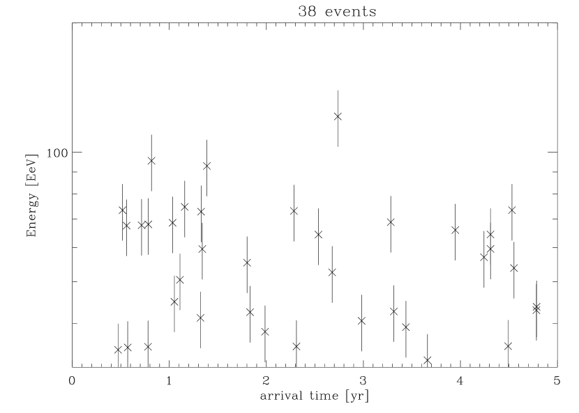
Figure 4: Same as Fig. 1, except for the parameters $\tau_{100}=0.1\,$yr, $T_{\rm S}=500\,$yr, and $N_{0}=4\times 10^{3}$. This serves as an example of a source that is continuously emitting at all relevant energies.

Main features of the time-energy images of clusters of UHE protons are described in detail in Ref.[24]. We summarize these results briefly, as they are important to the following. If both $T_{\rm S}<\tau_{100}$, and $\tau_{100}$ is small compared to $T_{\rm obs}$, arrival time and energy are correlated according to $\tau_{E}\propto E^{-2}$; see Fig. 1. A source, such that $\tau_{100}\gg T_{\rm S}$ and $\tau_{100}\gg T_{\rm obs}$, can be seen only in a limited range of energies, at a given time, as discussed in Ref.[23], as shown in Fig. 2,3. Below the GZK cut-off, the width of this stripe, in the time-energy plane and within the observational window of length $T_{\rm obs}$, is then tied to the ratio $D\theta_{E}/l_{c}$, as discussed above. At the other extreme, a source emitting continuously at all energies of interest here, i.e. with $T_{\rm S}\gg\tau_{30}$ and $T_{\rm S}\gg T_{\rm obs}$, yields a time-energy image in which the distribution of arrival time vs. energy is uniform, i.e. events of any energy can be recorded at any time, as shown in Fig. 4. Finally, for a source, such that $\tau_{100}<T_{\rm S}$ and $\tau_{30}>T_{\rm S}$, together with $T_{\rm S}\gg T_{\rm obs}$, there exists an energy $E_{\rm C}$, such that $\tau_{E_{\rm C}}=T_{\rm S}$. In this case, protons with an energy lower than $E_{\rm C}$ are not detected, as they could not have reached us within $T_{\rm obs}$, even if they were among the first emitted. However, protons with an energy higher than $E_{\rm C}$ are detected as for a continuously emitting source, i.e. with a uniform distribution of arrival times vs. energy, see Fig. 5.

Typical simulated clusters corresponding to these five main situations are shown in Figs. 1-5. The fluence $N_{0}$ was normalized in each case so that $\simeq 40$ events are expected within 5 years.

3 Maximum likelihood reconstruction

In this section, we discuss, in turn, how each parameter can be obtained from a likelihood study of UHE CR clusters. Certain marginalizations of Eq. (1) are used whenever the focus is only on one or a part of the parameters. The other parameters are then averaged or integrated over, applying weight functions (i.e., Bayesian priors) that represent the prior knowledge on their values. As we have currently no information on the fluence, the emission timescale $T_{\rm S}$ and the time delay $\tau_{E}$, the prior chosen would be uniform in the logarithm of these parameters. However, we note that the time delay $\tau_{E}$ is bounded from above by the Faraday rotation data bound on $B_{\rm rms}l_{c}^{1/2}$ as combined with Eq. (2). Moreover, information contained in the angular image should also be included in the prior on $\tau_{E}$, as $\tau_{E}\simeq D\theta_{E}^{2}/4$. The marginalization over the injection spectral index $\gamma$ is achieved through averaging with equal weights.

Although we focus on only one source, future large-scale experiments are expected to detect a large number of individual sources. Obviously, this would considerably increase the sensitivity to the physical parameters.

3.1 Time delay $\tau_{E}$

Here we assume that the source is a burst, i.e. $T_{\rm S}\ll 1\,$yr; we will discuss the case where $T_{\rm S}\gg 1\,$yr in the section concerning $T_{\rm S}$.

If the time delay is small compared to the length of the observational window, the time-energy correlation is scanned through, and, as Fig. 1 reveals, as simple fit of $\tau_{E}\propto E^{-2}$ would allow to determine the zero-point of emission, hence the time delay. This constitutes a measurement of the combination $DB_{\rm rms}l_{c}^{1/2}$. Our likelihood simulations confirm that, for the cluster shown in Fig. 1 for instance, $\tau_{E}$ is obtained within a factor 2. The source is found to be a burst with a high level of confidence.

When the time delay gets significantly larger than $T_{\rm obs}$, its actual value cannot be reconstructed from the maximum of the likelihood. This case corresponds to the clusters shown in Figs. 2 and 3. Indeed, the likelihood is degenerate in the parameters $N_{0}$ and $\tau_{100}$, as it depends mainly on the rate of detection $N_{0}/\Delta\tau_{100}$, where $\Delta\tau_{100}$ is the scatter in time around the mean of the $\tau_{E}-E$ correlation. As long as $N_{0}$ is unknown, only a lower limit to $\tau_{100}$, typically $\tau_{100}\mathrel{\mathchoice{\lower 3.6pt\vbox{\halign{$\mathsurround=0pt\displaystyle\hfil#\hfil$\cr>\crcr\sim\crcr}}}{\lower 3.6pt\vbox{\halign{$\mathsurround=0pt\textstyle\hfil#\hfil$\cr>\crcr\sim\crcr}}}{\lower 3.6pt\vbox{\halign{$\mathsurround=0pt\scriptstyle\hfil#\hfil$\cr>\crcr\sim\crcr}}}{\lower 3.6pt\vbox{\halign{$\mathsurround=0pt\scriptscriptstyle\hfil#\hfil$\cr>\crcr\sim\crcr}}}}T_{\rm obs}$, can be placed. The likelihood, as calculated for the cluster shown in Fig. 2, and marginalized over all parameters except $\tau_{100}$ and $\gamma$, is shown in Fig. 6 in order to illustrate this point. The distance and the coherence length cannot be readily obtained in this case, as we will discuss further below. Although only a lower limit could be placed on the time delay, we note that, when combined with the Faraday rotation bound, this would still allow to bracket the strength of the extra-galactic magnetic field, within less than a few orders of magnitude.

At this point, the information contained in the angular image of the source becomes important. If the angular image is not resolved, this translates into an upper limit on $\tau_{E}/D$, which may supersede the Faraday rotation bound, see Eq. (2), and Eq. (3) below. At the other extreme, for a sufficiently large time delay, $\theta_{E}$ should in principle be measurable, as

$$\theta_{E}\simeq 0.02^{\circ}\left(\frac{D}{10\,{\rm Mpc}}\right)^{-1/2}\left(\frac{\tau_{E}}{1\,{\rm yr}}\right)^{1/2}\,.$$ (3)

Obviously, resolving the angular image would change the prior for $D$ and $\tau_{100}$; it would sharpen the maximum likelihood reconstruction, notably with respect to the various scenarios discussed in Section 2. We have not included this angular effect in a systematic way; a quantitative treatment of the angular images will be the subject of a future study. We note that the angular resolutions of future UHE CR experiments are fractions of a degree, hence the information contained in the angular image becomes significant for $\tau_{100}\mathrel{\mathchoice{\lower 3.6pt\vbox{\halign{$\mathsurround=0pt\displaystyle\hfil#\hfil$\cr>\crcr\sim\crcr}}}{\lower 3.6pt\vbox{\halign{$\mathsurround=0pt\textstyle\hfil#\hfil$\cr>\crcr\sim\crcr}}}{\lower 3.6pt\vbox{\halign{$\mathsurround=0pt\scriptstyle\hfil#\hfil$\cr>\crcr\sim\crcr}}}{\lower 3.6pt\vbox{\halign{$\mathsurround=0pt\scriptscriptstyle\hfil#\hfil$\cr>\crcr\sim\crcr}}}}10\,$yr.

3.2 Distance $D$

As mentioned above, the distance enters the likelihood mainly through the amplitude of pion production. As long as the high energy tail of the spectrum, i.e. $E\mathrel{\mathchoice{\lower 3.6pt\vbox{\halign{$\mathsurround=0pt\displaystyle\hfil#\hfil$\cr>\crcr\sim\crcr}}}{\lower 3.6pt\vbox{\halign{$\mathsurround=0pt\textstyle\hfil#\hfil$\cr>\crcr\sim\crcr}}}{\lower 3.6pt\vbox{\halign{$\mathsurround=0pt\scriptstyle\hfil#\hfil$\cr>\crcr\sim\crcr}}}{\lower 3.6pt\vbox{\halign{$\mathsurround=0pt\scriptscriptstyle\hfil#\hfil$\cr>\crcr\sim\crcr}}}}50\,$EeV, can be observed, the distance is thus obtained with a reasonably good accuracy from the likelihood, as marginalized over $T_{\rm S}$, $\tau_{100}$, $N_{0}$, and $\gamma$. In particular, the likelihood is sensitive to the distance if the source has a large emission timescale, $T_{\rm S}\gg\tau_{100}$. The standard error is then roughly a factor $\simeq 2$. For example, the cluster of Fig. 4 shows a factor $\simeq 5$ difference in the marginalized likelihood for $50\,$Mpc (the true value) and $30\,$Mpc; such a factor is a typical value. The difference between $50\,$Mpc and $5\,$Mpc is typically a factor $\simeq 15$.

If $T_{\rm S}\ll\tau_{100}\mathrel{\mathchoice{\lower 3.6pt\vbox{\halign{$\mathsurround=0pt\displaystyle\hfil#\hfil$\cr<\crcr\sim\crcr}}}{\lower 3.6pt\vbox{\halign{$\mathsurround=0pt\textstyle\hfil#\hfil$\cr<\crcr\sim\crcr}}}{\lower 3.6pt\vbox{\halign{$\mathsurround=0pt\scriptstyle\hfil#\hfil$\cr<\crcr\sim\crcr}}}{\lower 3.6pt\vbox{\halign{$\mathsurround=0pt\scriptscriptstyle\hfil#\hfil$\cr<\crcr\sim\crcr}}}}T_{\rm obs}$, and the range of energies seen by the detector is above the GZK cut-off, the distance can still be evaluated, albeit with a somewhat larger error. Typical differences in the likelihood between 50 and $30\,$Mpc and 50 and $5\,$Mpc are factors $\simeq 2$ and $\simeq 6$, respectively.

In the intermediate case where $\tau_{100}$ and $T_{\rm S}$ are comparable, so that $\tau_{E_{\rm C}}=T_{\rm S}$ for an $E_{\rm C}$ in the observable energy range, the sensitivity to $D$ is the better the lower $E_{\rm C}$, albeit not very strong. The difference in the likelihood between $50\,$Mpc and $30\,$Mpc is typically a factor 3 or less (e.g., for the cluster shown in Fig. 5). It quickly rises, however, to a factor $\simeq 20$ for clusters of the order of 100 events. We note that, due to the comparatively limited energy range seen in this case, there is a partial degeneracy between $D$ and the injection spectrum parametrized by $\gamma$. For example, the marginalized likelihood does not change significantly if $D$ is decreased and $\gamma$ is increased (i.e. a softer injection spectrum is assumed) at the same time.

Other cases, e.g., as shown in Figs. 2 and 3, do not allow to reconstruct $D$.

3.3 Emission timescale $T_{\rm S}$

If the emission timescale is larger than the width of the observational window, the likelihood becomes degenerate in the ratio $N_{0}/T_{\rm S}$, and only a lower limit to $T_{\rm S}$ can be obtained, typically $T_{\rm S}\mathrel{\mathchoice{\lower 3.6pt\vbox{\halign{$\mathsurround=0pt\displaystyle\hfil#\hfil$\cr>\crcr\sim\crcr}}}{\lower 3.6pt\vbox{\halign{$\mathsurround=0pt\textstyle\hfil#\hfil$\cr>\crcr\sim\crcr}}}{\lower 3.6pt\vbox{\halign{$\mathsurround=0pt\scriptstyle\hfil#\hfil$\cr>\crcr\sim\crcr}}}{\lower 3.6pt\vbox{\halign{$\mathsurround=0pt\scriptscriptstyle\hfil#\hfil$\cr>\crcr\sim\crcr}}}}T_{\rm obs}$. However, if the time delay at some intermediate energy, between say $30\,$EeV and $100\,$EeV, is sufficiently large, and comparable to the emission timescale, then both the time delay, and the emission timescale, can be measured as long as a lower energy cut-off is visible above which the emission appears continuous. This case corresponds to the cluster shown in Fig. 5. Indeed, if the time delay is sufficiently large, then $\theta_{E}$ can be observationally measured according to Eq. (3). As discussed above, the likelihood has some sensitivity to the distance as long as events are observed over a reasonable range of energies. This sensitivity also depends strongly on the statistics of the UHE CR cluster. Since $\tau_{E}\simeq D\theta_{E}^{2}/4$, $\tau_{E}$ is obtained, and, as discussed in Ref.[24], the emission timescale corresponds to the time delay at the cut-off energy $E_{\rm C}$, below which no UHE CR are recorded within $T_{\rm obs}$, as follows from the definition of this lower cut-off energy, $\tau_{E_{\rm C}}=T_{\rm S}$.

In reality, however, the image observed in such a situation will appear as a burst with a large time delay most of the time: for $E<E_{\rm C}$, the image is similar to that of a burst with a large time delay, as $\tau_{E}>T_{\rm S}\gg T_{\rm obs}$, i.e. only a limited range in energies is detected. Because $\tau_{30}>\tau_{E_{\rm C}}$, most sources are seen at $E<E_{\rm C}$ rather than at $E>E_{\rm C}$, where the image is similar to that of a continuous source. Notably, the likelihood for a bursting source with $T_{\rm S}\simeq 0$ does not exclude the above intermediate situation, for a cut-off $E_{\rm C}$ above the observed stripe in the time-energy image of a bursting source. In the case of Fig. 7, corresponding to the cluster shown in Fig. 3, the stripe is observed between $\simeq 30\,$EeV and $\simeq 80\,$EeV, and the likelihood does not exclude the above intermediate case with $E_{\rm C}\mathrel{\mathchoice{\lower 3.6pt\vbox{\halign{$\mathsurround=0pt\displaystyle\hfil#\hfil$\cr>\crcr\sim\crcr}}}{\lower 3.6pt\vbox{\halign{$\mathsurround=0pt\textstyle\hfil#\hfil$\cr>\crcr\sim\crcr}}}{\lower 3.6pt\vbox{\halign{$\mathsurround=0pt\scriptstyle\hfil#\hfil$\cr>\crcr\sim\crcr}}}{\lower 3.6pt\vbox{\halign{$\mathsurround=0pt\scriptscriptstyle\hfil#\hfil$\cr>\crcr\sim\crcr}}}}80\,$EeV. Needless to say, the best reconstruction of $\tau_{100}$ and $T_{\rm S}$ takes place when the source is observed above $E_{\rm C}$, see Fig. 8.

Finally, note that if $T_{\rm S}\gg\tau_{30}$, the continuous source is hardly mistaken for a burst with a large time delay, which would be the closest approximation to the time-energy image of a continuous source. This can be seen in Fig. 9, which represents contours of the likelihood in the $\tau_{100}-T_{\rm S}$ plane. If the likelihood is further marginalized with respect to $T_{\rm S}$ or $\tau_{100}$ (see Fig. 10), a burst with a large time delay is ruled out to about 95% confidence level. Qualitatively speaking, the difference is that for a burst with a large time delay, the maximum fluence occurs at some intermediate energy, and the fluence decreases with decreasing energy below. For a continuous source, in contrast, the fluence increases with decreasing energy, according to the injection negative power law spectrum.

3.4 Injection spectrum index $\gamma$

The injection spectrum index $\gamma$ can be measured provided UHE CRs are recorded over a bandpass in energy that is sufficiently broad. More precisely, in the case of a continuous source, i.e. $T_{\rm S}\gg\tau_{30}$, $\gamma$ can be measured with an absolute accuracy of $\simeq 0.3$. This is based on the likelihood as marginalized over $T_{\rm S}$, $\tau_{100}$, and $N_{0}$, albeit for a known distance $D$. For example, for a continuously emitting source at $D=50\,$Mpc with $\gamma=2.0$ (see, e.g., Fig. 4), we obtained a difference in the likelihood for $\gamma=1.5$ and 2.5 of a factor of about 30 and 2, respectively, on average. An example for this situation is given in Fig. 10. In the case of a continuous source with a time delay comparable to the emission timescale, i.e. such as shown in Fig. 5, the respective factors are about 2 and 1, and therefore hardly significant. For a burst with a small time delay such as in Fig. 1 these factors are about 10 and 1. A burst with $\tau_{100}\gg T_{\rm obs}$ in which case the signal would be spread over a large range in energy, is even less sensitive to $\gamma$. In general, therefore, it is comparably easy to rule out a hard injection spectrum if the actual $\gamma\mathrel{\mathchoice{\lower 3.6pt\vbox{\halign{$\mathsurround=0pt\displaystyle\hfil#\hfil$\cr>\crcr\sim\crcr}}}{\lower 3.6pt\vbox{\halign{$\mathsurround=0pt\textstyle\hfil#\hfil$\cr>\crcr\sim\crcr}}}{\lower 3.6pt\vbox{\halign{$\mathsurround=0pt\scriptstyle\hfil#\hfil$\cr>\crcr\sim\crcr}}}{\lower 3.6pt\vbox{\halign{$\mathsurround=0pt\scriptscriptstyle\hfil#\hfil$\cr>\crcr\sim\crcr}}}}2.0$, but it is much harder to distinguish between $\gamma=2.0$ and 2.5.

Our analysis of the sensitivity to $\gamma$ was restricted to a fixed distance $D$, mainly because of CPU time limitations of the present serial version of our code. We expect that in the absence of information on $D$, an additional marginalization over $D$ would decrease the sensitivity to $\gamma$. In particular, we already mentioned at the end of Section 3.2, a degeneracy of the likelihood between $\gamma$ and $D$ for the intermediate case, where $T_{\rm S}$ and $\tau_{E_{\rm C}}$ are comparable.

3.5 Fluence $N_{0}$

Because of the degeneracy of the likelihood in $N_{0}/T_{\rm S}$ and/or $N_{0}/\Delta\tau_{100}$ for large timescales, it is in general not possible to reconstruct $N_{0}$. A possible exception is the case where all the particles are detected, i.e. $\tau_{100}\mathrel{\mathchoice{\lower 3.6pt\vbox{\halign{$\mathsurround=0pt\displaystyle\hfil#\hfil$\cr<\crcr\sim\crcr}}}{\lower 3.6pt\vbox{\halign{$\mathsurround=0pt\textstyle\hfil#\hfil$\cr<\crcr\sim\crcr}}}{\lower 3.6pt\vbox{\halign{$\mathsurround=0pt\scriptstyle\hfil#\hfil$\cr<\crcr\sim\crcr}}}{\lower 3.6pt\vbox{\halign{$\mathsurround=0pt\scriptscriptstyle\hfil#\hfil$\cr<\crcr\sim\crcr}}}}T_{\rm obs}$, and $T_{\rm S}\mathrel{\mathchoice{\lower 3.6pt\vbox{\halign{$\mathsurround=0pt\displaystyle\hfil#\hfil$\cr<\crcr\sim\crcr}}}{\lower 3.6pt\vbox{\halign{$\mathsurround=0pt\textstyle\hfil#\hfil$\cr<\crcr\sim\crcr}}}{\lower 3.6pt\vbox{\halign{$\mathsurround=0pt\scriptstyle\hfil#\hfil$\cr<\crcr\sim\crcr}}}{\lower 3.6pt\vbox{\halign{$\mathsurround=0pt\scriptscriptstyle\hfil#\hfil$\cr<\crcr\sim\crcr}}}}T_{\rm obs}$.

We take advantage of this section to detail slightly the marginalization procedure over $N_{0}$. In most cases we marginalized over the fluence analytically, noting that the dependence of the likelihood on $N_{0}$ can be written as

$$\ln{\cal L}=a\exp(x)+bx+c\,,$$ (4)

with $x\equiv\ln N_{0}$ and where $a$, $b$, and $c$ depend on all other parameters except $N_{0}$. This just follows from the fact that $\rho_{j}$ in Eq. (1) is proportional to $N_{0}$. By using the approximation

$$\ln{\cal L}(x)\simeq\ln{\cal L}_{\rm max}-\frac{b}{2}(x-x_{\rm max})^{2}$$ (5)

in terms of value ${\cal L}_{\rm max}$ and location $x_{\rm max}$ of the $N_{0}-$maximized likelihood, marginalizing over $N_{0}$ with a uniform prior for $\ln N_{0}$ then amounts to computing

$$\int_{-\infty}^{+\infty}dx{\cal L}(x)={\cal L}_{\rm max}\left(\frac{2\pi}{b}\right)^{1/2}\,.$$ (6)

3.6 Coherence length $l_{c}$

Our simulations confirm the suggestion of Ref.[23], that the main effect of $l_{c}$ on the angle-time-energy image comes through the relative size of the scatter around the $\theta_{E}-\tau_{E}-E$ correlations. For a time-energy image, if the source is continuous, with $T_{\rm S}\gg\tau_{30}$, the correlation between $\tau_{E}$ and $E$ is drowned in the uniform emission of particles within the timescale $T_{\rm S}$, and $l_{c}$ plays no role. The coherence length can therefore be estimated only when $\tau_{100}\gg T_{\rm S}$, and $\tau_{100}\gg T_{\rm obs}$. In this case, the signal corresponds to that shown in Figs. 2 and 3, and the width of the signal is related to the value of $D\theta_{E}/l_{c}$. The likelihood marginalized over $N_{0}$ and $\gamma$ for the cluster Fig. 3, assuming two different coherence lengths, $l_{c}\simeq 0.25\,$Mpc and $l_{c}\simeq 1\,$Mpc, is shown in Figs. 7 and 11. The qualitative behavior of these contour plots is the following. The actual value of $l_{c}$ used in simulating the cluster is $l_{c}\simeq 0.25\,$Mpc, so that the likelihood shown in Fig. 7 uses the correct value of $l_{c}$. The width of a stripe in the time-energy plance, is tied to the ratio $D\theta_{E}/l_{c}$, or, equivalently, to $(D\tau_{E})^{1/2}/l_{c}$. The likelihood shown in Fig. 11, assuming $l_{c}\simeq 1\,$Mpc, is thus similar to that corresponding to $l_{c}\simeq 0.25\,$Mpc, although it requires a comparatively larger (i.e. $\simeq(1/0.25)^{2}$ times larger) time delay to reproduce the large scatter in the stripe.

This demonstrates that for a broad observed energy dispersion, a large coherence length can be ruled out at least when some information on the distance $D$ and the deflection angle $\theta_{E}$, and thus on $\tau_{E}$, is available. In contrast, ruling out a small coherence length for a small observed energy dispersion is much harder, due to the nature of Poisson statistics.

As mentioned previously, provided $\tau_{E}\mathrel{\mathchoice{\lower 3.6pt\vbox{\halign{$\mathsurround=0pt\displaystyle\hfil#\hfil$\cr>\crcr\sim\crcr}}}{\lower 3.6pt\vbox{\halign{$\mathsurround=0pt\textstyle\hfil#\hfil$\cr>\crcr\sim\crcr}}}{\lower 3.6pt\vbox{\halign{$\mathsurround=0pt\scriptstyle\hfil#\hfil$\cr>\crcr\sim\crcr}}}{\lower 3.6pt\vbox{\halign{$\mathsurround=0pt\scriptscriptstyle\hfil#\hfil$\cr>\crcr\sim\crcr}}}}10^{4}\,$yr, $\theta_{E}$ can be directly measured. Note that the upper limit on the magnetic field strength, obtained through Faraday rotation measurements, implies $\tau_{E}\mathrel{\mathchoice{\lower 3.6pt\vbox{\halign{$\mathsurround=0pt\displaystyle\hfil#\hfil$\cr<\crcr\sim\crcr}}}{\lower 3.6pt\vbox{\halign{$\mathsurround=0pt\textstyle\hfil#\hfil$\cr<\crcr\sim\crcr}}}{\lower 3.6pt\vbox{\halign{$\mathsurround=0pt\scriptstyle\hfil#\hfil$\cr<\crcr\sim\crcr}}}{\lower 3.6pt\vbox{\halign{$\mathsurround=0pt\scriptscriptstyle\hfil#\hfil$\cr<\crcr\sim\crcr}}}}2\times 10^{5}\,{\rm yr}(D/10\,{\rm Mpc})^{2}(E/10\,{\rm EeV})^{-2}$. Whenever $\theta_{E}$ is measurable, the degeneracy of the likelihood, with respect to the width of the signal in energy, thus concerns only the ratio $D/l_{c}$. As we argued above, the likelihood itself is not sensitive to the distance if the mean energy of the signal lies below the GZK cut-off. If the mean energy lies above the GZK cut-off, then not only $\theta_{E}$ should not be measurable, but the width itself of the signal now arises from two very different effects: one due to the different trajectories followed by different UHE CRs through the magnetic field, another due to the pion production stochastic broadening of the signal; these effects cannot be easily disentangled. Hence, the only way this degeneracy between $D$ and $l_{c}$ could be broken is through the observation of an astrophysical counterpart to the source, or the source host, and the direct measurement of its distance.

Finally, the likelihood was found extremely insensitive to the index $n_{B}$ of the power spectrum of magnetic inhomogeneities.

4 Conclusions

We have presented a Monte-Carlo likelihood analysis of the potential of future large-scale UHE CR experiments to reconstruct the physical parameters of the source and of intervening magnetic fields, when the strength of the latter is sufficient ($B_{\rm rms}\mathrel{\mathchoice{\lower 3.6pt\vbox{\halign{$\mathsurround=0pt\displaystyle\hfil#\hfil$\cr>\crcr\sim\crcr}}}{\lower 3.6pt\vbox{\halign{$\mathsurround=0pt\textstyle\hfil#\hfil$\cr>\crcr\sim\crcr}}}{\lower 3.6pt\vbox{\halign{$\mathsurround=0pt\scriptstyle\hfil#\hfil$\cr>\crcr\sim\crcr}}}{\lower 3.6pt\vbox{\halign{$\mathsurround=0pt\scriptscriptstyle\hfil#\hfil$\cr>\crcr\sim\crcr}}}}10^{-12}\,$G) to affect the propagation of UHE CRs.

We discussed five generic situations of the time-energy images of UHE CRs, which we classify according to the values of the time delay $\tau_{E}$ induced by the magnetic field, the emission timescale of the source $T_{\rm S}$, as compared to the lifetime of the experiment. For each case, we simulated clusters of UHE CRs using the instrumental characteristics typical of future experiments such as the Telescope Array, the High Resolution Fly’s Eye, and most notably, the Pierre Auger Project. To this end we have simulated the emission, the propagation in an extra-galactic magnetic field, and the detection of clusters of UHE CRs. We then performed a Monte-Carlo likelihood analysis on these UHE CRs, and tried to reconstruct the physical parameters from the maximum of the likelihood. We simulated clusters of $\sim 40$ events, as the next generation experiments are expected to detect $\sim 20-100$ events per cluster if the clustering recently suggested by the AGASA experiment [3] is real.

In summary, the likelihood presents different degeneracies between different parameters, which complicates the analysis. As an example, the likelihood is degenerate in the ratios $N_{0}/T_{\rm S}$, or $N_{0}/\Delta\tau_{100}$, where $N_{0}$ is the total fluence, and $\Delta\tau_{100}$ is the spread in arrival time: these ratios represent rates of detection. Another example is given by the degeneracy between the distance $D$ and the injection energy spectrum index $\gamma$. Yet another is the ratio $(D\tau_{E})^{1/2}/l_{c}$, that controls the size of the scatter around the mean of the $\tau_{E}-E$ correlation. Therefore, in most general cases, values for the different parameters cannot be pinned down, and generally, only domains of validity are found.

We find that the distance to the source is obtained from the pion production signature, above the Greisen-Zatsepin-Kuzmin cut-off, when the emission timescale of the source dominates over the time delay. Since the time delay decreases with increasing energy, we find that the lower the energy $E_{\rm C}$, defined by $\tau_{E_{\rm C}}\simeq T_{\rm S}$, the higher the accuracy on the distance $D$. The error on $D$ is, in the best case, typically a factor 2, for one cluster of $\simeq 40$ events. In this case, where the emission timescale dominates over the time delay at all observable energies, information on the magnetic field is only contained in the angular image, which we did not systematically include into our likelihood analysis due to computational limits. A more detailed investigation of angular images will be presented separately in a forthcoming study. Qualitatively, the size of the angular image is proportional to $B_{\rm rms}(Dl_{c})^{1/2}$, whereas the structure of the image, i.e. the number of separate images, is controled by the ratio $D^{3/2}B_{\rm rms}/l_{c}^{1/2}$. Finally, the case where the time delay dominates over the emission timescale, with a time delay shorter than the lifetime of the experiment, also allows to estimate the distance with a reasonable accuracy.

The strength of the magnetic field can only be obtained from the time-energy image in this latter case because the angular image will not be resolvable. When the time delay dominates over the emission timescale, and is, at the same time, larger than the lifetime of the experiment, only a lower limit corresponding to this latter timescale, can be placed on the time delay, hence on the strength of the magnetic field. When combined with the Faraday rotation upper limit, this would nonetheless allow to bracket the r.m.s. magnetic field strength within a few orders of magnitude. Here as well, significant information is contained in the angular image.

The coherence length enters the ratio $(D\tau_{E})^{1/2}/l_{c}$ that controls the scatter around the mean of the $\tau_{E}-E$ correlation in the time-energy image. It can therefore be estimated from the width of this image, provided the emission timescale is dominated by $\tau_{E}$ (otherwise the correlation would not be seen), and some prior information on $D$ and $\tau_{E}$ is available.

As a concluding remark, we point out that the magnetic field, although it ’scrambles’ the images of UHE CRs, also brings extra-information. It not only leaves a signature of its own, it may also, in the case where the time delay becomes comparable to the emission timescale at some intermediate energy, allow an evaluation of the emission timescale of the source itself. There is therefore very important information hiding in the angle-time-energy images of UHE CRs, which could be exploited by future large-scale experiments.

Figure 1: A typical cluster of UHE CR above $\simeq 30\,$EeV in the time-energy plane. This cluster was produced by a discrete source at $D=50\,$Mpc with an emission time scale $T_{\rm S}\ll 1\,$yr (i.e. a burst), an average time delay of $\tau_{100}=0.3\,$yr, and with $N_{0}=40$. For the extra-galactic magnetic field, a power law index $n_{B}=0$ and a coherence length $l_{c}\simeq 1\,$Mpc was assumed. The error bars correspond to an energy resolution $\Delta E/E=0.14$. The top label indicates the number of events in the cluster.

Figure 2: Same as for Fig. 1, except for the parameters $\tau_{100}=50\,$yr, and $N_{0}=4\times 10^{3}$. This serves as an example for a burst with a long time delay, but still in the limit of small deflection, $D\theta_{E}/l_{c}\ll 1$, leading to a small detected energy dispersion.

Figure 3: Same as Fig. 1, except for the parameters $\tau_{100}=250\,$yr, $N_{0}=2\times 10^{4}$, and $l_{c}\simeq 0.25\,$Mpc. This serves as an example for a burst with a long time delay for intermediate deflection, $D\theta_{E}/l_{c}\sim 1$. The distinct sub-bands are due to multiple source images.

Figure 5: Same as Fig. 1, except for the parameters $\tau_{100}=50\,$yr, $T_{\rm S}=200\,$yr, and $N_{0}=6\times 10^{3}$. A lower cut-off in energy occurs at $E_{\rm C}\simeq 50\,$EeV where $\tau_{E_{\rm C}}\simeq T_{\rm S}$.

Figure 6: The likelihood for the cluster shown in Fig. 2, marginalized over $T_{\rm S}$ and $N_{0}$, plotted versus the time delay $\tau_{100}$, for $D=50\,$Mpc and $l_{c}\simeq 1\,$Mpc (the true values). The solid line is for $\gamma=1.5$, the dotted for $\gamma=2.0$ (the true value), and the dashed line for $\gamma=2.5$. As a result, $\tau_{100}>5\,$yr to about 90% confidence level. In this case there is clearly no sensitivity to $\gamma$, as expected.

Figure 7: The likelihood for the cluster shown in Fig. 3, marginalized over $N_{0}$ and $\gamma$, plotted in the $\tau_{100}-T_{\rm S}$ plane, for $D=50\,$Mpc and $l_{c}\simeq 0.25\,$Mpc (the true values). The maximum of the likelihood occurs for $\tau_{100}\simeq$ a few hundred years, $T_{\rm S}\simeq$ a few years which is a good reconstruction of the true values. The contours shown go from the maximum down to values of about 0.01 of the maximum in steps of a factor $10^{0.2}=1.58$. Note that values in the range $\tau_{E}=T_{\rm S}$ with $E\mathrel{\mathchoice{\lower 3.6pt\vbox{\halign{$\mathsurround=0pt\displaystyle\hfil#\hfil$\cr>\crcr\sim\crcr}}}{\lower 3.6pt\vbox{\halign{$\mathsurround=0pt\textstyle\hfil#\hfil$\cr>\crcr\sim\crcr}}}{\lower 3.6pt\vbox{\halign{$\mathsurround=0pt\scriptstyle\hfil#\hfil$\cr>\crcr\sim\crcr}}}{\lower 3.6pt\vbox{\halign{$\mathsurround=0pt\scriptscriptstyle\hfil#\hfil$\cr>\crcr\sim\crcr}}}}80\,$EeV and $T_{\rm S}\mathrel{\mathchoice{\lower 3.6pt\vbox{\halign{$\mathsurround=0pt\displaystyle\hfil#\hfil$\cr>\crcr\sim\crcr}}}{\lower 3.6pt\vbox{\halign{$\mathsurround=0pt\textstyle\hfil#\hfil$\cr>\crcr\sim\crcr}}}{\lower 3.6pt\vbox{\halign{$\mathsurround=0pt\scriptstyle\hfil#\hfil$\cr>\crcr\sim\crcr}}}{\lower 3.6pt\vbox{\halign{$\mathsurround=0pt\scriptscriptstyle\hfil#\hfil$\cr>\crcr\sim\crcr}}}}10\,$yr are not significantly excluded, as expected (see text). The fall-off at $\tau_{100}\mathrel{\mathchoice{\lower 3.6pt\vbox{\halign{$\mathsurround=0pt\displaystyle\hfil#\hfil$\cr>\crcr\sim\crcr}}}{\lower 3.6pt\vbox{\halign{$\mathsurround=0pt\textstyle\hfil#\hfil$\cr>\crcr\sim\crcr}}}{\lower 3.6pt\vbox{\halign{$\mathsurround=0pt\scriptstyle\hfil#\hfil$\cr>\crcr\sim\crcr}}}{\lower 3.6pt\vbox{\halign{$\mathsurround=0pt\scriptscriptstyle\hfil#\hfil$\cr>\crcr\sim\crcr}}}}50\,$yr and $T_{\rm S}\mathrel{\mathchoice{\lower 3.6pt\vbox{\halign{$\mathsurround=0pt\displaystyle\hfil#\hfil$\cr<\crcr\sim\crcr}}}{\lower 3.6pt\vbox{\halign{$\mathsurround=0pt\textstyle\hfil#\hfil$\cr<\crcr\sim\crcr}}}{\lower 3.6pt\vbox{\halign{$\mathsurround=0pt\scriptstyle\hfil#\hfil$\cr<\crcr\sim\crcr}}}{\lower 3.6pt\vbox{\halign{$\mathsurround=0pt\scriptscriptstyle\hfil#\hfil$\cr<\crcr\sim\crcr}}}}3\,$yr is a numerical artifact due to the limited number of propagated particles ($4\times 10^{4}$ per parameter set) which causes too patchy histograms in arrival time.

Figure 8: Same as Fig. 7, but for the cluster shown in Fig. 5, and assuming $l_{c}\simeq 1\,$Mpc (the true value). The maximum of the likelihood is near $\tau_{100}=4\,$yr, $T_{\rm S}=100\,$yr, but any values along the ridge defined by $T_{\rm S}\simeq\tau_{50}$ are roughly equally likely, as expected from the fact that $E_{\rm C}\simeq 50\,$EeV (see Fig. 5 and text).

Figure 9: Same as Fig. 7, but for the cluster shown in Fig. 4, and assuming $l_{c}\simeq 1\,$Mpc (the true value). The maximum of the likelihood is near $\tau_{100}=0.1\,$yr, $T_{\rm S}=10^{3}\,$yr which is a good reconstruction of the true values. Parameters in the range $T_{\rm S}\mathrel{\mathchoice{\lower 3.6pt\vbox{\halign{$\mathsurround=0pt\displaystyle\hfil#\hfil$\cr<\crcr\sim\crcr}}}{\lower 3.6pt\vbox{\halign{$\mathsurround=0pt\textstyle\hfil#\hfil$\cr<\crcr\sim\crcr}}}{\lower 3.6pt\vbox{\halign{$\mathsurround=0pt\scriptstyle\hfil#\hfil$\cr<\crcr\sim\crcr}}}{\lower 3.6pt\vbox{\halign{$\mathsurround=0pt\scriptscriptstyle\hfil#\hfil$\cr<\crcr\sim\crcr}}}}10\,$yr and $\tau_{100}\mathrel{\mathchoice{\lower 3.6pt\vbox{\halign{$\mathsurround=0pt\displaystyle\hfil#\hfil$\cr>\crcr\sim\crcr}}}{\lower 3.6pt\vbox{\halign{$\mathsurround=0pt\textstyle\hfil#\hfil$\cr>\crcr\sim\crcr}}}{\lower 3.6pt\vbox{\halign{$\mathsurround=0pt\scriptstyle\hfil#\hfil$\cr>\crcr\sim\crcr}}}{\lower 3.6pt\vbox{\halign{$\mathsurround=0pt\scriptscriptstyle\hfil#\hfil$\cr>\crcr\sim\crcr}}}}10\,$yr, that would be typical for a burst with a large time delay, are excluded at about 95% confidence level (see text).

Figure 10: The likelihood for the cluster shown in Fig. 4, marginalized over $\tau_{100}$ and $N_{0}$, plotted versus the emission timescale $T_{\rm S}$, for $D=50\,$Mpc and $l_{c}\simeq 1\,$Mpc (the true values). The average over the curves shown for $\gamma=1.5$ (solid line), $\gamma=2.0$ (dotted line; the true value), and for $\gamma=2.5$ (dashed line), therefore, corresponds to a marginalization of the likelihood shown in Fig. 9 over $\tau_{100}$. This demonstrates even more clearly that $T_{\rm S}\mathrel{\mathchoice{\lower 3.6pt\vbox{\halign{$\mathsurround=0pt\displaystyle\hfil#\hfil$\cr<\crcr\sim\crcr}}}{\lower 3.6pt\vbox{\halign{$\mathsurround=0pt\textstyle\hfil#\hfil$\cr<\crcr\sim\crcr}}}{\lower 3.6pt\vbox{\halign{$\mathsurround=0pt\scriptstyle\hfil#\hfil$\cr<\crcr\sim\crcr}}}{\lower 3.6pt\vbox{\halign{$\mathsurround=0pt\scriptscriptstyle\hfil#\hfil$\cr<\crcr\sim\crcr}}}}10\,$yr is ruled out at about 95% confidence level.

Figure 11: Same as Fig. 7, but assuming a magnetic field coherence length $l_{c}\simeq 1\,$Mpc. The maximum of the likelihood is near $\tau_{100}=400\,$yr, $T_{\rm S}=20\,$yr which again is a reasonable reconstruction of the true values. Note that if $\tau_{100}$ were known to be smaller than $\simeq 50\,$yr, a coherence length as large as $l_{c}=7\,$Mpc could be ruled out, but $l_{c}\simeq 0.25\,$Mpc would be allowed (see Fig. 7 and discussion in the text).

References

- [1] M. A. Lawrence, R. J. O. Reid, and A. A. Watson, J. Phys. G Nucl. Part. Phys. 17 (1991) 733.
- [2] N. Hayashida et al., Phys. Rev. Lett. 73 (1994) 3491; S. Yoshida et al., Astropart. Phys. 3 (1995) 105.
- [3] N. Hayashida et al., Phys. Rev. Lett 77 (1996) 1000.
- [4] D. J. Bird et al., Phys. Rev. Lett. 71 (1993) 3401; Astrophys. J. 424 (1994) 491; ibid. 441 (1995) 144.
- [5] T. Stanev et al., Phys. Rev. Lett. 75 (1996) 3056.
- [6] K. Greisen, Phys. Rev. Lett. 16 (1966) 748; G. T. Zatsepin and V. A. Kuzmin, Pis’ma Zh. Eksp. Teor. Fiz. 4 (1966) 114 [JETP. Lett. 4 (1966) 78].
- [7] J. W. Elbert and P. Sommers, Astrophys. J. 441 (1995) 151.
- [8] F. Halzen, R. A. Vazques, T. Stanev, and H. P. Vankov, Astropart. Phys. 3 (1995) 151.
- [9] J. L. Puget, F. W. Stecker, and J. H. Bredekamp, Astrophys. J. 205 (1976) 638; F. W. Stecker, e-print astro-ph/9710353.
- [10] G. Sigl and S. Lee, in Proc. 24th International Cosmic Ray Conference (Istituto Nazionale Fisica Nucleare, Rome, 1995) Vol. 3, 356.
- [11] J. P. Rachen and P. L. Biermann, Astron. Astrophys. 272 (1993) 161.
- [12] E. Waxman, Phys. Rev. Lett. 75 (1995) 386.
- [13] E. Waxman, Astrophys. J. 452 (1995) L1.
- [14] M. Vietri, Astrophys. J. 453 (1995) 883.
- [15] M. Milgrom and V. Usov, Astrophys. J. 449 (1995) L37.
- [16] E. Waxman, Proc. of International Symposium on Extremely High Energy Cosmic Rays: Astrophysics and Future Observatories (Institute for Cosmic Ray Research, Tokyo, 1996), p. 114.
- [17] P. Bhattacharjee, C. T. Hill, and D. N. Schramm, Phys. Rev. Lett. 69 (1992) 567.
- [18] C. T. Hill, Nucl. Phys. B 224 (1983) 469.
- [19] G. Sigl, Space Sc. Rev. 75 (1996) 375.
- [20] P. P. Kronberg, Rep. Prog. Phys. 57 (1994) 325.
- [21] R. Plaga, Nature 374 (1995) 430.
- [22] E. Waxman, and P. Coppi, Astrophys. J. 464 (1996) L75.
- [23] E. Waxman and J. Miralda-Escudé, Astrophys. J. 472 (1996) L89.
- [24] M. Lemoine, G. Sigl, A. V. Olinto, and D.N. Schramm, Astrophys. J., 486 (1997) L115.
- [25] S. Lee, A. V. Olinto, and G. Sigl, Astrophys. J. 455 (1995) L21.
- [26] G. Sigl, M. Lemoine, A.V. Olinto, Phys. Rev. D 56 (1997) 4470.
- [27] Proc. of International Symposium on Extremely High Energy Cosmic Rays: Astrophysics and Future Observatories (Institute for Cosmic Ray Research, Tokyo, 1996).
- [28] S. C. Corbató et al., Nucl. Phys. B (Proc. Suppl.) 28B (1992) 36; M. Al-Seady et al., in [27], p. 191.
- [29] M. Teshima et al. Nucl. Phys. B (Proc. Suppl.) 28B (1992) 169; M. Hayashida et al., in [27], p. 205.
- [30] J. W. Cronin, Nucl. Phys. B (Proc. Suppl.) 28B (1992) 213; The Pierre Auger Observatory Design Report (2nd ed.) 14 March 1997.
- [31] J. F. Ormes et al., in Proc. 25th International Cosmic Ray Conference (Durban, 1997), eds.: M. S. Potgieter et al., 5, 273; Y. Takahashi et al., in [27], p. 310.
- [32] M. J. Chodorowski, A. A. Zdziarski, and M. Sikora, Astrophys. J. 400 (1992) 181.