CMB Anisotropy Correlation Function and Topology from Simulated Maps for MAP

Abstract

We have simulated cosmic microwave background (CMB) anisotropy maps for several $COBE$-DMR-normalized cold dark matter (CDM) cosmogonies, to make predictions for the MAP experiment, an upcoming whole-sky CMB anisotropy space mission. We have studied the sensitivity of the simulated MAP data to cosmology, sky coverage, and instrumental noise. Given an accurate knowledge of instrumental noise, MAP data will ably discriminate amongst the cosmogonies considered, and superbly determine the topology of the initial fluctuations.

A correlation function analysis of the simulated MAP data results in a very accurate measurement of the acoustic Hubble radius at decoupling. A low-density open CDM model with $\Omega_{0}=0.4$ can be distinguished from the $\Omega_{0}=1$ fiducial CDM model or a spatially-flat CDM model with a cosmological constant and $\Omega_{0}=0.4$ with more than 99% confidence from the location of the acoustic “valley” in the correlation function.

A genus analysis of the simulated MAP data indicates that in cosmogonies with Gaussian random-phase initial conditions, the horizontal shift of the zero-crossing point of the genus curve near the mean temperature threshold level $\nu=0$ should not exceed $|\Delta\nu|=0.01$ (0.04) when the total effective FWHM smoothing is $0.3{{}^{\circ}}$ $(1.0{{}^{\circ}})$. The asymmetry of the genus curve at the positive and negative threshold levels should not exceed $|\Delta g/g(\nu=\pm 1)|=0.8\%$ (4%) at $0.3{{}^{\circ}}$ $(1{{}^{\circ}})$ FWHM smoothing. Deviations of the observed MAP data in excess of these small values will be evidence for non-Gaussian behavior.

The amplitude of the genus curve is a measure of the shape of the power spectrum at the smoothing scale. Even with the expected amount of instrumental noise and partial sky coverage (due to the Galaxy), the MAP data should allow discrimination amongst the cosmogonies considered at more than 99% confidence solely from a genus amplitude analysis.

1 Introduction

Following the $COBE$-DMR detection of anisotropy in the cosmic microwave background on large angular scales (Smoot et al. 1992; Wright et al. 1992; Bennett et al. 1996; Górski et al. 1996), there have been many measurements of CMB anisotropy on angular scales down to $\sim 10^{\prime}$ (Ganga et al. 1994; Gutiérrez et al. 1997; Piccirillo et al. 1997; Netterfield et al. 1997; Gundersen et al. 1995; Tucker et al. 1997; Platt et al. 1997; Masi et al. 1996; Lim et al. 1996; Cheng et al. 1997; Griffin et al. 1997; Scott et al. 1996; Leitch et al. 1997; Church et al. 1997, see Page 1997 for a review). In addition to the DMR experiment, CMB anisotropy maps have been produced from four other experiments (Ganga et al. 1994; White & Bunn 1995; Scott et al. 1996; Tegmark et al. 1997). CMB anisotropy observations are beginning to test cosmogonical models and provide interesting constraints on cosmological parameters in these models (e.g., Bunn & Sugiyama 1995; Górski et al. 1995, 1998; Stompor, Górski, & Banday 1995; Ganga, Ratra, & Sugiyama 1996; Ganga et al. 1997a,b, 1998; Hancock et al. 1997; Bond & Jaffe 1997; Stompor 1997; Lineweaver & Barbosa 1997; Ratra et al. 1997b). However, definitive results, including significant constraints on cosmological parameters, must await new CMB anisotropy data, covering a large fraction of the sky (to minimize sample variance) and acquired at a variety of frequencies (to allow for control over possible non-CMB anisotropy foreground contamination). Of the currently available data sets, the DMR maps best meet these criteria.

Plans are afoot to launch two second-generation CMB anisotropy satellite missions — the Microwave Anisotropy Probe (MAP) is expected to have data in less than four years, and the Planck Surveyor is expected to have data in less than a decade. These missions are expected to measure the CMB anisotropy on angular scales larger than a fraction of a degree, at a variety of frequencies. MAP will probe the anisotropy at frequencies of 22, 30, 40, 60, and 90 GHz at expected angular resolutions of 0.93, 0.68, 0.47, 0.35, and 0.21 degrees (FWHM beamwidths), respectively. At 90 GHz the MAP sensitivity is expected to be $\sim 35\ \mu$K per $0.3^{\circ}\times 0.3^{\circ}$ pixel. Planck Surveyor is expected to measure the CMB anisotropy at frequencies ranging from 30 to 900 GHz with angular resolution ranging from 0.5 to 0.075 degrees.

It is now possible to make accurate predictions for the CMB anisotropy, as a function of cosmological parameters, in many different cosmological models. In conjunction with such theoretically computed model CMB anisotropy spectra, the data from these experiments should lead to an accurate determination of cosmological parameters, such as the mass density parameter $\Omega_{0}$, the baryonic-mass density parameter $\Omega_{B}$, the cosmological constant ${\Lambda}$, the Hubble parameter $H_{0}$, the matter power spectrum, and the optical depth to the last scattering surface (e.g., Spergel 1994; Jungman et al. 1996; Bond, Efstathiou, & Tegmark 1997; Zaldarriaga, Spergel, & Seljak 1997; Dodelson, Kinney, & Kolb 1997). At the least, the data from these space missions should in principle be able to rule out most cosmological models currently under consideration. The present situation in cosmology — where one is able to make definite theoretical predictions which can be judged by near-future observations — is quite unusual.

Prior to the $COBE$-DMR measurement of the large-scale CMB anisotropy, Gott et al. (1990) had generated simulated all-sky CMB anisotropy maps predicted in the spatially-flat $\Omega_{0}=1$ fiducial CDM model with Gaussian, adiabatic, scale-invariant matter fluctuations. The DMR data is indeed consistent with such a CMB anisotropy spectrum (Górski et al. 1996, 1998).

In this paper we generate simulated all-sky CMB anisotropy maps appropriate for MAP in several representative cosmological models normalized to the DMR data. Our predictions can be directly compared to the MAP data when it is available. Hinshaw, Bennett, & Kogut (1995) have generated all-sky CMB anisotropy maps expected in an $\Omega_{0}=1$ CDM model, at angular resolutions of $0.5^{\circ}$ and $1^{\circ}$, to study the effects of sky coverage, angular resolution, instrumental noise, and unresolved features in the data. Novikov & Jørgensen (1996) have simulated $10^{\circ}\times 10^{\circ}$ sky anisotropy maps of $\Omega_{0}=1$ CDM models with $\Omega_{B}=0.1$ and 0.03 at $0.5^{\circ}$–$1^{\circ}$ resolutions. They have examined various statistical properties of the temperature fluctuation field, such as clustering of peaks and percolation. We focus here on generating mock CMB anisotropy maps appropriate for the specific experimental configuration of MAP. We also use these CMB anisotropy maps to examine the ability of the expected MAP data to discriminate between different cosmological models. In what follows we assume that the MAP data will be limited by statistical noise rather than foregrounds or systematic errors.

In Section 2 we present the cosmological models we study, and explain how the simulated CMB anisotropy maps are generated. In Section 3 we compute the CMB anisotropy correlation function for each of the simulated maps, and show that it is sensitive to the acoustic peaks in the CMB anisotropy angular power spectrum. In Section 4 we study the genus statistic of the generated maps, and explore its ability to discriminate between cosmological models and to detect non-Gaussian fluctuations in the CMB anisotropy field. The effect of instrumental noise is considered. Conclusions follow in Section 5.

2 Simulation of CMB Anisotropy Maps

To generate simulated CMB anisotropy maps for MAP we have chosen four representative Gaussian, adiabatic cosmogonical models, with distinct CMB anisotropy angular power spectra: (1) The fiducial CDM model (FCDM) with $\Omega_{0}=1$, the Hubble parameter $H_{0}$ divided by 100 km/sec/Mpc $h=0.5$, and with no reionization. (2) A spatially-flat, low-density CDM model ($\Lambda$CDM) with a cosmological constant $\Lambda$, $\Omega_{0}=0.4$, and $h=0.6$. (3) A spatially-open low-density CDM model (OCDM) with no $\Lambda$, $\Omega_{0}=0.4$, and $h=0.65$. (4) A reionized fiducial CDM model (RCDM) with $\Omega_{0}=1$, $h=0.5$, and fully reionized at redshift $z=100$ (i.e., with electron ionization fraction $x_{e}=1$ at $z\leq 100$ and so optical depth $\tau=1$). For all models, the baryonic-mass density parameter is $\Omega_{B}=0.0125h^{-2}$. Further details are given in Ratra et al. (1997a) and Sugiyama (1995).

The FCDM and $\Lambda$CDM models considered here assume a scale-invariant primordial energy-density power spectrum (Harrison 1970; Peebles & Yu 1970; Zel’dovich 1972), as is predicted in the simplest spatially-flat inflation models (Guth 1981, also see Kazanas 1980; Sato 1981). The FCDM model is inconsistent with galaxy clustering data (e.g., Maddox et al. 1990; Saunders et al. 1991; Vogeley et al. 1992; Park et al. 1994), but still serves as a useful fiducial for cosmological model comparison. $\Lambda$CDM models (Peebles 1984) became popular when it was discovered that the large-scale galaxy distribution was of the form expected in CDM models with $\Omega_{0}h\sim 0.2-0.3$ (e.g., Park 1990, 1991; Vogeley et al. 1992; da Costa et al. 1994; Peacock & Dodds 1994), since these models could be accommodated in the then-dominant spatially-flat inflation scenario. However, an open inflating universe can also be created as a single bubble during the decay of an initial metastable inflation state (Gott 1982, 1986). The OCDM model considered here assumes the primordial energy-density power spectrum of the simplest open-bubble inflation models (Ratra & Peebles 1994, 1995; Bucher, Goldhaber, & Turok 1995; Yamamoto, Sasaki, & Tanaka 1995). The low-density models, OCDM and $\Lambda$CDM, are consistent with most current large-scale structure and CMB anisotropy observations (e.g., Gott 1997; Turner 1997; Cole et al. 1997; Gardner et al. 1997; Croft et al. 1997; Coles et al. 1997; Jenkins et al. 1997).

A CMB temperature fluctuation field on the surface of a sphere (i.e., the sky) can be decomposed into a sum of spherical harmonics, ${\delta T/T}(\theta,\phi)=\sum a^{m}_{\ell}Y_{\ell}^{m}(\theta,\phi)$, where $(\theta,\phi)$ are the angular coordinates on the sky. If the initial matter fluctuation is a Gaussian random field, as predicted in simple inflation models, the expansion coefficients $a^{m}_{\ell}$ are independent Gaussian random variables with zero means and variances $\langle|a^{m}_{\ell}|^{2}\rangle=C_{\ell}$, where $C_{\ell}$ is the CMB anisotropy angular power spectrum (see below for more details).

The CMB anisotropy angular power spectra of the four models considered here are shown in Figure 1 (Ratra et al. 1997a; Sugiyama 1995). Following Górski et al. (1998) and Stompor (1997), the angular power spectra are normalized to the arithmetic mean of the $\pm$2-$\sigma$ $COBE$-DMR 53 and 90 GHz data from the two extreme data sets: (1) galactic-frame maps accounting for the high-latitude Galactic emission correction and including the $\ell=2$ moment in the analysis; and (2) ecliptic-frame maps ignoring the high-latitude Galactic emission correction and excluding the $\ell=2$ moment from the analysis.

At large angular scales the CMB anisotropy angular power spectra in the four models are of approximately the same amplitude. At smaller angular scales acoustic oscillations due to the pressure of the photon-baryon fluid and matter velocity perturbations at photon decoupling cause the angular power spectra to rise. At still smaller angular scales photon diffusion and the finite thickness of the last-scattering surface smears out the fluctuations. These effects give rise to the characteristic acoustic peaks in the angular power spectra on intermediate angular scales. In an open model the geometrical effect that the circumference of a circle is larger than $2\pi$ times its radius moves these peaks to smaller angular scales relative to the spatially-flat case (Kamionkowski, Spergel, & Sugiyama 1994). In the spatially-flat $\Omega_{0}=1$ FCDM and low-density $\Lambda$CDM models, the first acoustic peak is at $\ell=217$ and $\ell=222$, respectively. The amplitudes of the peaks in these models are different. In the open case the first peak is at $\ell=349$, while in the reionized RCDM model the peaks are smeared out. Consequently, the presence, location, and amplitude of the acoustic peaks are a valuable probe of the geometry and content of the universe.

In real observations and analyses, the temperature fluctuations on the sky are convolved with the beam pattern of the experiment, and are often further smoothed to increase the signal-to-noise ratio. If the beam pattern is $B(\theta)$ and the smoothing filter is $F(\theta)$, the observed CMB anisotropy temperature field is

$${\delta T\over T}(\theta,\phi)=\sum_{\ell=2}^{\infty}\sum_{m=-\ell}^{\ell}a^{m}_{\ell}Y_{\ell}^{m}(\theta,\phi)B_{\ell}F_{\ell},$$ (1)

where $B_{\ell}$ and $F_{\ell}$ are the coefficients of the beam pattern and the smoothing filter expanded in Legendre polynomials, and we consider only harmonics higher than the dipole. Assuming the idealized case of an all-sky data map, the inverse relation for the harmonic amplitude is

$$a_{\ell}^{m}=\int d\Omega{\delta T\over T}(\theta,\phi)Y_{\ell}^{m}(\theta,\phi)^{*}/B_{\ell}F_{\ell}.$$ (2)

For a Gaussian beam (or a smoothing filter) with a width $\lambda\ll 1$ to a very good approximation,

$$B_{\ell}=\exp(-(\ell+1/2)^{2}\lambda^{2}/2).$$ (3)

We use equation (1) to simulate the CMB anisotropy maps for MAP. We limit the summation to $\ell\leq 1500$. For each cosmogony the real and imaginary components of $a^{m}_{\ell}$ are randomly sampled Gaussian variates with zero means, and variances equal to $C_{\ell}/2$ for the $m\neq 0$ harmonics and equal to $C_{\ell}$ for the $m=0$ harmonics. We adopt a Gaussian beam with FWHM $\theta_{B}=0.21^{\circ}$ (or width $\lambda=\theta_{B}/2\sqrt{2\ln 2}$ in equation [3]). The temperature fluctuations are then computed at $1801\times 3600$ points in ($\theta,\phi$) space on a grid with $0.1^{\circ}$ spacing.

The data from MAP is expected to include instrumental noise of $\sim 35$ $\mu$K per $0.3^{\circ}\times 0.3^{\circ}$ pixel. If the noise is white, its power spectrum is constant $C_{\ell}\equiv C_{N}$. Consider a pure noise map convolved with a top hat filter $F$ with area of 0.09 square degrees. Then the variance of the noise temperature fluctuation, which is set to $(35\ \mu$K$/T_{0})^{2}$ per 0.09 square degrees, is given by equation (5) below (at $\theta=0$ with $C_{\ell}$ replaced by $C_{N}$). The top hat filter is $F(\theta)=1/\pi\theta_{H}^{2}$ for $\theta\leq\theta_{H}$, and $0$ otherwise. The coefficients of its expansion into Legendre polynomials are, for $\theta_{H}\ll 1$,

$$F_{\ell}=\sum_{n=0}^{\infty}{(-)^{n}\over(n!)^{2}(n+1)}[(\ell+1/2)\theta_{H}/2]^{2n}.$$ (4)

We obtain from equation (5) $C_{N}=5\times 10^{-15}$ for MAP. One can study the effects of noise on statistics using this noise power spectrum. In practice, of course, the MAP results will include an estimate of the noise at each pixel derived from the many observations taken as the satellite’s horns sweep out complicated paths on the sky. The satellite horns are paired, so subtracting their signals gives the noise map; this allows an extremely accurate characterization of the noise as a function of position on the sky. Such a detailed noise map will allow a much more careful accounting of instrumental noise. (For example, the noise at the ecliptic poles is expected to be about half of that at the ecliptic plane).

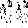
Figure 8: Threshold masks from a subset (approximately $30{{}^{\circ}}\times 30{{}^{\circ}}$) of the OCDM CMB anisotropy simulations at $1.0{{}^{\circ}}$ FWHM smoothing: ($a$) ignoring instrumental noise, ($b$) accounting for instrumental noise (rms noise $=35\ \mu$K per $0.3{{}^{\circ}}\times 0.3{{}^{\circ}}$ area).

The maps resulting from the $\Lambda$CDM and OCDM models with simulated (constant over the sky) instrumental noise, projected according to the Mollweide projection method (Snyder 1993), are shown in Figure 2 (Plate 1). These maps are smoothed with a $0.214{{}^{\circ}}$ FWHM Gaussian, which makes the total smoothing scale of the signal $0.3{{}^{\circ}}$. The Mollweide equal area projection shows the whole sky in a single map, but structures are distorted. In the topology study we use conformal stereographic projection maps where shapes of structures are preserved locally. Stereographic maps of the CMB fluctuations simulated for the OCDM and $\Lambda$CDM models and convolved with a $0.978{{}^{\circ}}$ FWHM Gaussian (which makes the total smoothing scale of the signal $1.0{{}^{\circ}}$) are shown in Figure 3 (Plate 2). At this smoothing length most structures in the map generated by MAP will correspond to actual CMB anisotropy fluctuations (see Figure 8). It is to be noted that the OCDM and $\Lambda$CDM maps are visually very similar — this is a consequence of the expected instrumental noise and smoothing (see Figures 1$b$ and 1$c$). We emphasize, however, that this does not mean that MAP can not statistically distinguish between these models.

3 Correlation Function

Differences between cosmological models are often displayed in terms of the angular power spectrum, as in Figure 1. Most models have relatively small differences at large scales ($\ell\leq 30$), but they often have relatively large differences at small scales ($\ell\geq 100$). The structure of the acoustic peaks at smaller angular scales depends on the cosmogony and the cosmological parameters. Hence, to test cosmogonies and measure these parameters, it is essential to have an accurate measurement of the location and amplitude of the acoustic peaks. Note that the acoustic peaks cause an oscillatory wave in the power spectrum (see Figure 1). Furthermore, the amplitudes of individual harmonics in the power spectrum are destined to fluctuate with respect to the mean. To measure precisely the amplitude and location of the acoustic peaks in the power spectrum one must make a fit over many harmonics.

An important integral of the power spectrum is the two-point auto-correlation function, the real-space Fourier counterpart of the power spectrum. Since the hot and cold spots due to the acoustic peaks in the power spectrum are compact in real space (their size is fixed by the acoustic Hubble radius at decoupling — see Figures 2 and 3), it is useful to explore them in real space. (Note that in Fourier space the peaks are well-approximated by a wavy sinc-function.) While the correlation function and the power spectrum are simply related, it is useful to analyze data both in real space and in Fourier space (e.g., Hinshaw et al. 1996; Górski et al. 1996; Wright et al. 1996).

The correlation function of CMB temperature fluctuations, corresponding to equation (1), is

$$C(\theta)={1\over 4\pi}\sum_{\ell=2}^{\infty}C_{\ell}(2\ell+1)P_{\ell}(\cos\theta)B_{\ell}^{2}F_{\ell}^{2}.$$ (5)

Here $P_{\ell}$ are Legendre polynomials and we have ignored the monopole and dipole harmonics. The power spectra shown in Figure 1$a$ can be approximated by an exponential minus a sinc-function. For example, the acoustic peaks of the FCDM power spectrum can be approximately described by the function $-{\rm sinc}(4.5\ell/\ell_{max})$. Consequently, these acoustic peaks should appear as a negative top hat in the correlation function.

Figure 4 shows the correlation functions of the four models considered. Thick curves are the correlation functions transformed from the power spectrum curves in Figure 1. Thin solid curves, tracing the thick ones at large angular separations, account for the convolution with a $0.21^{\circ}$ Gaussian beam in Figure 4$a$ and with additional $0.214^{\circ}$ Gaussian smoothing in Figure 4$b$. The acoustic peaks in the power spectrum indeed appear as a valley in this plot. The position, depth, and width of the acoustic valley depend on the model and the cosmological parameters. We have generated seven sets of $a_{\ell}^{m}$’s for the FCDM model, and have computed their correlation functions. These are also plotted, using dots, in Figure 4. At separations $\geq 1^{\circ}$ cosmic variance causes a large scatter amongst the seven correlation functions. Hence it is very difficult to discriminate between models using large angular scale data alone. However, direct measurement from these realizations shows that the FCDM acoustic valley in the function $\theta^{1/2}C(\theta)$ is consistently located at $\theta=1.13^{\circ}\pm 0.02^{\circ}$, comparing excellently with the theoretically predicted FCDM acoustic valley location at $\theta=1.13^{\circ}$ for a $0.21^{\circ}$ beam (and at $1.17^{\circ}$ in the unsmoothed map). The OCDM model acoustic valley lies at a smaller separation of $0.65^{\circ}\pm 0.03^{\circ}$ ($0.69^{\circ}$ in the unsmoothed map) — clearly distinguishable from the acoustic valleys of the FCDM and $\Lambda$CDM models (some 13-$\sigma$ difference for the fixed cosmological parameter values used here).

On the other hand, the spatially-flat FCDM and $\Lambda$CDM models have acoustic peaks at nearly the same angular scales. Therefore, they have to be differentiated by the amplitude of the power spectrum or the correlation function. It can be noted from Figure 4 that the correlation functions of the FCDM and $\Lambda$CDM models are statistically significantly different at separations $\theta\approx 0.5^{\circ}$. In the case of an ideal sample with whole-sky coverage and with no noise, the MAP data would distinguish the correlation function of the FCDM universe from that of the $\Lambda$CDM case at the 2.6-$\sigma$ level at angular separations near $\theta=0.5^{\circ}$. Note that this ignores the relative uncertainty between the DMR normalizations of the FCDM and $\Lambda$CDM models. The numerical value of this relative uncertainty is not known, however, the absolute model-dependent uncertainty in the DMR normalization is $\sim 10$–$12\%$ (in $Q_{\rm rms-PS}$, the quadrupole amplitude of the CMB anisotropy, Górski et al. 1998). Also note that, for this comparison between FCDM and $\Lambda$CDM, cosmological parameters such as $h$ and $\Omega_{B}$ are held fixed.

To estimate the effects of instrumental noise on the correlation function analysis of the MAP data we use the noise power spectrum, $C_{N}=5\times 10^{-15}$, derived above. This noise power is added to the CMB anisotropy signal, and the map is then further smoothed with a $0.214{{}^{\circ}}$ FWHM Gaussian. That is, we generate a set of $(a_{\ell}^{m}B_{\ell}+n)F_{\ell}$ up to $\ell=2500$ where $n$ is a Gaussian random variable with zero mean and $\langle n^{2}\rangle=C_{N}$, and $B_{\ell}$ and $F_{\ell}$ represent the $0.21{{}^{\circ}}$ beam and $0.214{{}^{\circ}}$ smoothing filter, respectively. The corresponding correlation function is then computed. From seven realizations of the noise-added correlation functions for FCDM and OCDM the positions of the acoustic valleys are measured to be at $\theta=1.13{{}^{\circ}}\pm 0.03{{}^{\circ}}$ and $0.65{{}^{\circ}}\pm 0.04{{}^{\circ}}$, respectively. The correlation function acoustic valleys of the FCDM and OCDM models are now 9-$\sigma$ apart. It is also noted (from Figure 4) that the statistical uncertainty in the amplitude of correlation function at separations $\theta\geq 0.5{{}^{\circ}}$ is hardly affected by the instrumental noise expected for MAP. This means that cosmic variance, rather than instrumental noise, dominates the statistical uncertainty in the correlation function at these scales. (This is also true for the genus statistic — see Table 1.) Therefore, the above argument on discrimination between the spatially-flat models on the basis of the amplitude of the correlation function remains essentially unchanged.

4 Topology

The power spectrum and correlation function measured from the observed CMB anisotropy maps provides important information on the nature of density fluctuations in the early universe, thus constraining structure formation mechanisms. Another important statistical characteristic of a CMB anisotropy map is whether or not its temperature fluctuation field is Gaussian random-phase. One can test for Gaussianity of the temperature distribution by constructing histograms of the pixel values. To test the Gaussianity and phase properties of the maps the genus topology test is useful. In this section we study the topology of the CMB anisotropy isotemperature contour surfaces. This provides information on the global structure of the density fluctuation field.

4.1 The Genus

The genus has been used as a measure of topology of the matter/galaxy distribution. For three-dimensional topology see Gott, Melott, & Dickinson (1986), Gott, Weinberg, & Melott (1987), Vogeley et al. (1994), and Cole et al. (1997); for two-dimensional topology see Melott et al. (1989), Park et al. (1992), and Colley (1997). The genus has also been used as a measure of the topology of CMB anisotropy fields (Coles 1988; Park & Gott 1988; Gott et al. 1990; Colley, Gott, & Park 1996; Kogut et al. 1996; Schmalzing & Górski 1997; Winitzki & Kosowsky 1997). For the two-dimensional CMB anisotropy temperature field, the genus is the number of hot spots minus the number of cold spots, i.e., at a temperature threshold level $\nu$ the genus is

$$g(\nu)={1\over 2\pi}\int_{C}\kappa ds,$$ (6)

where $\kappa$ is the signed curvature of the isotemperature contours $C$. The genus curve as a function of the temperature threshold level has a characteristic shape for a Gaussian random-phase field. Changing the shape of the CMB anisotropy power spectrum only changes the amplitude of the genus curve. Hence the genus curve provides a good measure of both non-random phases and the shape of the power spectrum. The above real-space definition of the genus allows it to be directly used for studying the statistics of the acoustic peak hot and cold spots. Previous measurements of the CMB anisotropy genus (see references above) were consistent with the Gaussian random-phase hypothesis.

The theoretical genus per steradian of a two dimensional Gaussian field with correlation function $C(\theta)$ is (Gott et al. 1990)

$$g(\nu)={1\over(2\pi)^{3/2}}{C^{(2)}\over C^{(0)}}\nu e^{-\nu^{2}/2},$$ (7)

where $C^{(n)}\equiv(-)^{n/2}(d^{n}C/d\theta^{n})_{\theta=0}$, and the threshold temperature fluctuation is $\nu\sqrt{C^{(0)}}=\nu\sigma$. For a CMB anisotropy temperature map convolved with beam $B$ and smoothing filter $F$, $C^{(0)}$ and $C^{(2)}$ are given by

$$C^{(0)} = {1\over 4\pi}\sum(2\ell+1)C_{\ell}B_{\ell}^{2}F_{\ell}^{2}$$ (8)

$$C^{(2)} = {1\over 8\pi}\sum\ell(\ell+1)(2\ell+1)C_{\ell}B_{\ell}^{2}F_{\ell}^{2},$$ (9)

where we have used the relation $P_{\ell}^{\prime}(1)=\ell(\ell+1)/2$ (see equation [5]). The genus per steradian is then

$$g(\nu)={1\over 2(2\pi)^{3/2}}{\sum\ell(\ell+1)(2\ell+1)C_{\ell}B_{\ell}^{2}F_{\ell}^{2}\over\sum(2\ell+1)C_{\ell}B_{\ell}^{2}F_{\ell}^{2}}\nu e^{-\nu^{2}/2}.$$ (10)

We note again that the genus curve shape is fixed by the Gaussian random-phase nature of the field, and its amplitude depends only on the shape of the CMB anisotropy power spectrum and not on its amplitude.

For scale-free energy-density perturbations with matter power spectrum $P(k)=\langle|\delta_{k}|^{2}\rangle=Ak^{n}$ in a spatially-flat universe, the CMB anisotropy angular power spectrum is (Peebles 1982; Bond & Efstathiou 1987)

$$C_{\ell}={2^{n-1}A\over(2c/H_{o})^{n+3}}{\Gamma(3-n)\over\Gamma^{2}({4-n\over 2})}{\Gamma({2\ell+n-1\over 2})\over\Gamma({2\ell+5-n\over 2})}.$$ (11)

We can estimate the slope of the CMB anisotropy power spectrum near the smoothing scale from the amplitude of the genus curve by using equation (10) and this formula.

4.2 Topology of the MAP Simulations

When the MAP data becomes available one can measure the genus of the observed CMB anisotropy and so constrain cosmological models and structure formation mechanisms. Here we use our simulated CMB anisotropy maps to study the sensitivity of the genus statistic to models in the presence of instrumental noise and when the sky coverage is incomplete.

We use the stereographic projection to map the CMB anisotropy sky simulations onto a plane. The stereographic projection is conformal and preserves local geometry. For a hemisphere the projection is defined by

$$\rho=2\tan\left({{\pi/2-|b|}\over 2}\right);~{}~{}\phi=\ell,$$ (12)

where $\rho$ is the radius and $\phi$ is the position angle in the projected plane, $b$ is galactic latitude and $\ell$ is galactic longitude (and should not be confused with the Legendre polynomial index). Figure 3 (Plate 2) shows such projections for the OCDM and $\Lambda$CDM simulations.

When computing the genus we exclude regions with $|b|<30{{}^{\circ}}$ to excise the Galactic plane region where the Galactic signal is likely to be important. We use the method of Gott et al. (1990) to compute the topology of the proper planar projection of the simulated CMB anisotropy sky. In Figure 5 points with error bars show the two-dimensional genus topology, at $1.0^{\circ}$ FWHM smoothing, derived from the simulated MAP data (accounting for noise). The error bars are formal errors in the mean derived from the variance among the genus measurements in each of the eight octants of the sphere. The curves show the function $g=N\nu e^{-\nu^{2}/2}$, the form expected for a random-phase Gaussian field, where $N$ has been adjusted to fit the points optimally via the least-squares method. For goodness of fit, the points along the curves should be compared with Student’s $t$-variates, rather than Gaussian variates, since the error bars have been estimated from the data themselves (rather than independently). Following Gott et al. (1990) and Colley (1997), we use the variable

$$\tilde{\chi}^{2}=\sum_{i=1}^{21}{{(\bar{g}_{i}-{g_{i,{\rm fit}})^{2}}\over{{s_{i}}^{2}}/(n-1)}}$$ (13)

to estimate the goodness of fit. The sum runs over the 21 $\nu$ values at which the genus $g_{i}$ is computed; $\bar{g}_{i}$ is the mean genus among the eight octants of the sphere and $s_{i}{}^{2}$ is the variance. We find for the OCDM case $\tilde{\chi}^{2}=23.6$, and for FCDM $\tilde{\chi}^{2}=26.3$. Since $\tilde{\chi}^{2}$ does not follow a $\chi^{2}$ distribution, due to the non-Gaussian distributions of the $g_{i}$’s, we generate $10^{4}$ Monte Carlo runs of $\tilde{\chi}^{2}$ variables with 20 degrees of freedom, and 8 samplings within each degree of freedom, exactly as we expect in equation (13) (since we have fit one parameter, the amplitude). In each run, we generate 8 independent ($\mu=0,\sigma=1$) Gaussian variates within 20 independent groups. From the eight samples in each group $i$ we estimate the mean ($\bar{g}_{i}$) and the standard deviation in the mean $s_{i}/\sqrt{n-1}$; $\bar{g}_{i}/(s_{i}/\sqrt{n-1})$ is thus a ($\mu=0,\sigma=1$) $t$-variate. In the $10^{4}$ Monte Carlo simulations, we compute $\tilde{\chi}^{2}$ as in equation (13), by summing the squares of the twenty $t$-variates. We find that the $\tilde{\chi}^{2}$ values of 23.6 and 26.3 fall at the 43% and 54% levels of the cumulative distribution of the $10^{4}$ simulated $\tilde{\chi}^{2}$ variables, demonstrating an excellent agreement with the theoretical curve.

In addition to noise, several non-CMB anisotropy foregrounds could contaminate the MAP data. Perhaps the foreground of most consequence for the genus analysis is the radio point-source background (mainly AGNs). To assess its significance, we have added point sources to the $0.3{{}^{\circ}}$ FWHM smoothed OCDM map. These point sources (also smoothed) are taken to have a number distribution in flux, $f$, given by $dN(f)=kf^{-2.5}df$. The normalization $k$ is chosen to reflect the real sky and has an average of one source at 3 $\mu$K or brighter per $0.3{{}^{\circ}}\times 0.3{{}^{\circ}}$ pixel (Holdaway, Owen, & Rupen 1994). Comparing to the OCDM map with noise alone, we find that the point sources introduce an rms scatter in $g(\nu)$ of 23 (relative to the point-source-free map), significantly smaller than the typical uncertainty in $g(\nu)$, which is 42 in the map without point sources. We have also compared the genus values (between the maps with and without point sources) using the $\chi^{2}$ statistic. We find $\chi^{2}=2.8$ out of an expected 21 (21 $\nu$ values), confirming that the effect of the point sources on the genus is very small. Since larger smoothing lengths would diminish the signal from point sources even further (as with the noise), we conclude that the effects of the point-source foreground on the genus are small.

Galactic foregrounds, including warm dust and free-free emission, have been selected against in choosing the frequency coverage of MAP. At the optimum frequencies, these foregrounds are expected to be nearly an order of magnitude smaller than the CMB anisotropy. Furthermore, in the analysis of the DMR data (Bennett et al. 1996; Górski et al. 1996, and references therein) the $COBE$-DIRBE 140 $\mu$m sky map (Reach et al. 1995) was used to correct for dust and free-free emission contamination, and the 408 MHz all-sky radio survey (Haslam et al. 1982) was used to correct for synchrotron emission contamination. A similar approach, strengthened by new all-sky survey data, should (hopefully) suffice for dealing with these contaminants in the MAP data.

Another possible foreground is the Sunyaev-Zel’dovich effect in clusters of galaxies (Sunyaev & Zel’dovich 1972). Here hot electrons Compton scatter the CMB photons to uniformly higher frequency, introducing an apparent decrease in brightness temperature as great as $\sim 1$ mK on the few arc-minute scale (for very massive clusters with a velocity dispersion of $\sim 1000$ km/s, Markevitch et al. 1992). At smoothing lengths of $0.3{{}^{\circ}}$ and higher, the effect is reduced to $\sim 10\ \mu$K, significantly below the peaks in the CMB anisotropy (see Figure 2). Also, X-ray surveys of hot gas in the intracluster medium can be used to locate the massive clusters causing the shift, and to help estimate the expected magnitude of the shift (e.g., Klein et al. 1991). (In the MAP data, the large Sunyaev-Zel’dovich signal will come from the Coma cluster; this region can be excised from the analysis. This signal can also be estimated by projecting the thermal fluctuations out of the two highest frequency MAP channels. A combination of these cuts should be able to remove most of the Sunyaev-Zel’dovich contamination from the MAP data.)

Non-Gaussian features in the CMB anisotropy will affect the genus curve in many different ways. Here we consider two cases that can be quantified. Non-Gaussianity can shift the observed genus curve to the left (towards negative thresholds) or right, near the mean threshold level. It can also alter the amplitudes of the genus curve at positive and negative levels differently, causing $|g(\nu=1)|\neq|g(\nu=-1)|$. The direction and degree of shift and asymmetry of the genus curve depend on the number, size and height/depth of hot and cold spots. We have computed limits on these non-Gaussianity measures from our simulated maps. In the FCDM model we find that the MAP data will detect a shift of the genus curve near $\nu=0$ (the five $\nu$ values in Figure 5 centered on $\nu=0$) for $|\Delta\nu|>0.01\ (0.04)$ for FWHM smoothing of $0.3{{}^{\circ}}\ (1.0{{}^{\circ}})$; the limits are the 2-$\sigma$ error bars derived from the variances between fits for $\Delta\nu$ from the eight octants. The asymmetry of the genus amplitude near $\nu=\pm 1$ (the five $\nu$ values centered on 1 and $-1$) can be detected for $|\Delta g/g(\nu=\pm 1)|>0.8\%\ (4\%)$ at $0.3{{}^{\circ}}\ (1{{}^{\circ}})$ FWHM smoothing (also 2-$\sigma$). The limits for $|\Delta\nu|$ and $|\Delta g/g(\nu=\pm 1)|$ are very similar for OCDM and $\Lambda$CDM.

4.3 Genus Amplitude as a Check of Cosmological Model

From Figure 5, it is clear that the amplitude of the genus curves for FCDM and OCDM differ significantly. We first consider the genus amplitude for the case when instrumental noise is ignored. In the four cosmogonies considered, and in the scale-invariant power-law model, we expect from equation (10) a theoretical genus per steradian of $g(\nu=1)=101.0\pm 6.2$ (FCDM), $115.4\pm 6.9$ ($\Lambda$CDM), $74.3\pm 6.6$ (OCDM), $45.2\pm 3.9$ (RCDM), and $44.4\pm 3.9$ ($n=1$ scale-invariant power-law model), when the total smoothing scale (by the beam and the filter) is $1{{}^{\circ}}$ FWHM. The uncertainty limits here account for cosmic variance, computed from actual realizations of $a_{\ell}^{m}$’s. Note that these limits are computed from the Galactic-plane-excluded maps. Also, since the genus amplitude does not depend on the amplitude of the CMB anisotropy angular power spectrum, these results are insensitive to the uncertainty in the DMR normalization of the models.

We have also computed the genus directly from simulated maps that include receiver noise, for a single realization of each model. (Since all the model computations use the same random number seed, the cosmic variance effect is minimal.) In Figure 6 we have plotted these genus amplitudes at $\nu=1$ for the FCDM, OCDM and $\Lambda$CDM models. For comparison, we have also plotted the genus for the same cosmogonical simulations but now ignoring noise. In the inset, we have zoomed in on the values at $0.3{{}^{\circ}},0.5{{}^{\circ}}$ and $1.0{{}^{\circ}}$ total FWHM smoothing, with 1-$\sigma$ error bars derived from comparison of the fits to the genus values within each of the eight octants (these error bars agree very well with the $\Delta\chi^{2}=1$ level, as expected, c.f. Press et al. 1992). We have listed in Table 1 the genus values, with statistical uncertainty and expected cosmic variance, from Figure 6. Note that the $0.3{{}^{\circ}}$ column values are subject to finite pixelization of both the model MAP results and the projected maps (Melott et al. 1989). Tests have shown that amplitude ratios between models remain very nearly constant when moving to higher resolution in the projected maps. Hence, it is the finite pixelization of our simulations which ultimately limits the resolution for the genus computation.

The three cosmogonies of Figure 6 and Table 1 have significantly different genus amplitudes, even when the expected instrumental noise is accounted for. They can thus be discriminated between on the basis of the genus amplitude. For instance, at the $0.3{{}^{\circ}}$ smoothing scale each model is distinguished from the other two at greater than 6-$\sigma$ confidence (Table 1 and we have added all error bars in quadrature). (We again emphasize that the other cosmological parameters, such as $h$ and $\Omega_{B}$, are not allowed to vary in these models.) These results may be directly compared to the genus measurements from MAP, as an independent check of the results inferred from the power spectrum and correlation function analyses.

4.4 Effects of Noise on the Genus

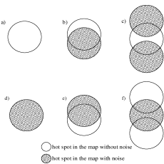
Figure 7: Overlays of simulated maps with and without instrumental noise. This schematic illustrates the effect of noise on the genus by comparing how well a given structure in the map with noise corresponds to a structure in the noise-free map. If a structure in the map with noise, such as a hot spot, intersects exactly one hot spot in the noise-free map, as in cases $b$) and $e$), then the noise has not altered the genus. However, if the noise is significant, artificial hot spots can appear or real hot spots can disappear, both of which would alter the genus. $a$) is a case where the noise has removed a hot spot (there is a hot spot in the noise-free map but not in the map with noise), $c$) where the noise has split a hot spot into two. $d$) is a case where the noise has added a hot spot (there is a hot spot in the map with noise but not in the noise-free map), $f$) where the noise has merged two hot spots into one.

In order to understand more completely the effects of receiver noise on the genus, we can look in detail at what is happening, structure by structure, when noise is added. At a high temperature cut, for instance, noise can add a hot spot by adding a small amount of positive temperature to a region near the cut; conversely, noise can remove a small hot spot by cooling a high-temperature region to below the cut. We have illustrated schematically in Figure 7 the possible effects of noise on the genus. In Figure 7$b$ and 7$e$ the noise has neither added nor subtracted hot spots, leaving the genus unaltered. In Figure 7$a$, however, the noise has removed a hot spot and reduced the genus by one; in 7$c$ the noise has split a hot spot into two and added one to the genus. In Figure 7$d$ the noise has added an artificial hot spot and one to the genus while in 7$f$ the noise has merged two hot spots into one and reduced the genus by one. These splittings and mergings can occur in higher multiples.

We now examine our simulated maps for these effects. In Figure 8$a$ we have plotted the $\nu=1$ threshold mask for a subsection of the noiseless OCDM $1.0{{}^{\circ}}$ FWHM smoothed map. In Figure 8$b$ we have plotted the same mask, but for a map with noise added. Several of the structures in Figure 8$a$ become subdivided in Figure 8$b$ — noise has split hot spots. Also, several new hot spots appear, while at least one cold spot (in the upper right) develops within a hot spot. To understand these changes quantitatively, we have counted the number of times each case in Figure 7 arises for the OCDM simulations of Figure 8. Results from this analysis are given in Table 2.

Table 2 shows that about 80% (660 out of [78+660+64+15+2+2]) of the structures counted in the noise-free map correspond to exactly one structure in the map with noise. 78 real hot spots occur with no corresponding hot spots in the map with noise, while 83 (=64+15+2+2) overlap two or more hot spots in the map with noise. Very similar correspondence exists in comparing the noise-added map hot spots to the noise-free map hot spots, except in the “0” column. About a quarter (249 out of [249+683+13+2+1]) of the hot spots in the map with noise had no corresponding hot spots in the noise-free map. This is to be expected because the noise adds artificial small-scale bumps on top of the signal. These bumps can push a pixel that was just below the threshold (here $\nu=1$) to a value over the threshold, so that extra hot spots appear (similarly, extra cold spots appear at $\nu=-1$). At $1.0{{}^{\circ}}$ FWHM smoothing about two-thirds (683 out of 1011) of the structures in the simulated MAP maps are due to real signal. Therefore most $1.0{{}^{\circ}}$ scale structures in the MAP maps will correspond to real fluctuations in the microwave background.

5 Conclusions

In this paper we have generated mock CMB anisotropy maps of representative DMR-normalized CDM cosmogonies appropriate for the MAP satellite experiment. We have studied the sensitivity of the simulated MAP data to cosmology, sky coverage, and instrumental noise. An accurate knowledge of instrumental noise is essential if the statistical tests considered here are to live up to expectations.

We have focused on the correlation function and the genus statistic as tests of cosmogonical models. If the underlying theory has Gaussian random phases, then these two statistics are just integrals of the power spectrum. However, since they are computed from the data in a very different manner than the power spectrum, they will be useful checks on power spectrum computations even in Gaussian random phase models. The genus statistic will also be a powerful test of the random phase hypothesis.

The correlation function statistic provides an accurate measurement of the acoustic Hubble radius at decoupling from the simulated MAP data. The $\Omega_{0}=0.4$ OCDM model considered here can be distinguished from the spatially-flat FCDM and $\Lambda$CDM models with more than 99% confidence from the location of the acoustic valley in the correlation function, even when the expected amount of instrumental noise is present. The FCDM and $\Lambda$CDM models can also be distinguished at separations $\sim 0.5{{}^{\circ}}$ by the amplitude of the correlation function. Note however that for these models all other cosmological parameters (such as $\Omega_{B}$ and $h$) are fixed.

The genus of the CMB fluctuations can also be accurately measured from the MAP data. The genus curves of Gaussian cosmological models allow a 2-$\sigma$ statistical horizontal shift of the zero-crossing point by only $|\Delta\nu|\lesssim 0.01\ (0.04)$ when the total effective smoothing is $0.3{{}^{\circ}}\ (1{{}^{\circ}})$ FWHM. The asymmetry of the genus curve at the positive and negative threshold levels is only $|\Delta g/g(\nu=\pm 1)|\lesssim 0.8\%\ (4\%)$ in the Gaussian cosmogonies considered. Deviations of the observed MAP data that exceed these values will be evidence for non-Gaussian behavior.

The amplitude of the genus curve, which is a measure of the shape of the power spectrum at the smoothing scale, can also be a powerful discriminator between cosmological models. Even with the expected amount of instrumental noise and partial sky coverage, the MAP data should discriminate between the cosmogonies considered here at confidence levels exceeding 99% just on the basis of the genus amplitude analysis.

Of possible outcomes from the MAP experiment, a more interesting one would be if the results were in close agreement with the low-$\Omega_{0}$ open-bubble inflation model. Not only would this tell us the value of $\Omega_{0}$, but it would affirm inflation and support the open-bubble inflation model in particular, thus providing evidence that there are universes other than our own (other bubble universes), all arising out of an initial metastable inflation state.

Table 1: Numerical values for genus amplitude per steradian at $\nu=1$

Smoothing scale	FCDM	OCDM	$\Lambda$CDM
$0.3{{}^{\circ}}$	$3650\pm 16\pm 23$	$3995\pm 21\pm 40$	$3313\pm 14\pm 22$
$0.5{{}^{\circ}}$	$637.6\pm 6.0\pm 13.6$	$719.1\pm 8.2\pm 22.1$	$617.9\pm 5.2\pm 14.0$
$1.0{{}^{\circ}}$	$137.7\pm 2.5\pm 6.2$	$120.9\pm 2.6\pm 6.6$	$149.7\pm 2.5\pm 6.9$

Table 2: Effects of noise on the genus

	intersecting hot spots
map1 $\rightarrow$ map2	0	1	2	3	4	5	6
noise-free $\rightarrow$ noise	78	660	64	15	2	2	0
noise $\rightarrow$ noise-free	249	683	63	13	2	1	0
change of genus	-1	0	1	2	3	4	5

Figure 1: Curves show the CMB anisotropy angular power spectra, as a function of multipole $\ell$, of the four models considered: FCDM (solid), ${\Lambda}$CDM (dotted), OCDM (dashed), and RCDM (long dashed). $T_{0}$ is the mean CMB temperature. The clouds of dots, tracing the curves at small $\ell$, are from actual realizations of the $a_{\ell}^{m}$’s with $0.21{{}^{\circ}}$ FWHM beam smoothing as appropriate for MAP, and show the cosmic variance at each $\ell$. The clouds of dots in panel ($a$) do not account for instrumental noise, while those in panels ($b$) and ($c$) do. The dots in the last two panels correspond to $0.3{{}^{\circ}}$ and $1.0{{}^{\circ}}$ total smoothing of the signal, respectively.

Figure 2: Upper panel is a Mollweide projection of the CMB anisotropy map simulated for the OCDM model. The map has been convolved by a Gaussian filter with $0.3{{}^{\circ}}$ FWHM. Lower panels are magnifications of the Mollweide projection of the simulated CMB anisotropy maps for the OCDM and $\Lambda$CDM models. In each lower panel map the equator runs horizontally through the center, where the plots cover $30{{}^{\circ}}$ horizontally and $24.4{{}^{\circ}}$ vertically.

Figure 3: Upper panel is the OCDM CMB anisotropy map, in stereographic projection and with $1{{}^{\circ}}$ FWHM Gaussian smoothing, showing the north and south galactic caps ($|b|>30{{}^{\circ}}$). The projection is conformal and the shape of structures are locally undistorted. Lower panel is a similar stereographic projection for the $\Lambda$CDM model. For the purpose of this comparison both models have identical phases, in both signal and noise (picked from the same random number seeds).

Figure 4: Correlation functions of the four cosmogonies. Thick curves are the correlation functions transformed from the power spectra shown with curves in Figure 1. Thin solid curves, tracing the thick ones at large angular separations, account for the convolution with a $0.21^{\circ}$ Gaussian beam in panel ($a$), with an additional $0.214^{\circ}$ Gaussian smoothing in panel ($b$). Dotted curves are the correlation functions from seven independent realizations of FCDM CMB anisotropy skies showing the cosmic variance. Thin solid and dotted curves in panel ($a$) ignore instrumental noise, while those in panel ($b$) account for it. The Galactic-plane cut is not accounted for. Clearly, inclusion of instrumental noise smoothed over a small scale ($\sim$ beam size) does not change the correlation function much, indicating that the statistical uncertainty is dominated by cosmic variance.

Figure 5: Two-dimensional genus topology from the MAP simulations accounting for instrumental noise, with $1.0^{\circ}$ FWHM smoothing and for $|b|>30{{}^{\circ}}$. Open symbols are for OCDM, closed for FCDM. Error bars are derived from the variance of the genus computed independently in each of the eight octants of the sphere. The curves show the functional form expected for a random-phase Gaussian field, $N\nu e^{-\nu^{2}/2}$, and have been fit to the points by adjusting $N$. The cosmogonies can clearly be distinguished from each other.

Figure 6: Fit amplitudes (at $\nu=1$) of genus curves for various cosmogonies, as in Figure 5. Filled squares are results from noise-free maps for FCDM, filled triangles for $\Lambda$CDM, and filled circles for OCDM. Open squares are results from maps with noise for FCDM, open triangles for $\Lambda$CDM, and open circles for OCDM. The error bars shown in the insets are the quadrature sum of the statistical uncertainty and that due to cosmic variance (see Table 1).

References

- Banday et al. (1997) Banday, A. J., Górski, K. M., Bennett, C. L., Hinshaw, G., Kogut, A., Lineweaver, C., Smoot, G. F., & Tenorio, L. 1997, ApJ, 475, 393
- Bennett et al. (1996) Bennett, C. L., et al. 1996, ApJ, 464, L1
- Bond & Efstathiou (1987) Bond, J. R., & Efstathiou, G. 1987, MNRAS, 226, 655
- Bond, Efstathiou, & Tegmark (1997) Bond, J. R., Efstathiou, G., & Tegmark, M. 1997, MNRAS, in press
- Bond & Jaffe (1997) Bond, J. R., & Jaffe, A. 1997, in Microwave Background Anisotropies, ed. F. R. Bouchet, R. Gispert, B. Guiderdoni, & J. Tran Thanh Van (Gif-sur-Yvette: Editions Frontieres), 197
- Bucher, Goldhaber, & Turok (1995) Bucher, M., Goldhaber, A. S., & Turok, N. 1995, Phys. Rev. D, 52, 3314
- Bunn & Sugiyama (1995) Bunn, E. F., & Sugiyama, N. 1995, ApJ, 446, 49
- Cheng et al. (1997) Cheng, E. S., et al. 1997, ApJ, 488, L59
- Church et al. (1997) Church, S. E., Ganga, K. M., Ade, P. A. R., Holzapfel, W. L., Mauskopf, P. D., Wilbanks, T. M., & Lange, A. E. 1997, ApJ, 484, 523
- Cole et al. (1997) Cole, S., Weinberg, D. H., Frenk, C. S., & Ratra, B. 1997, MNRAS, 289, 37
- Coles (1988) Coles, P. 1988, MNRAS, 234, 509
- Coles et al. (1997) Coles, P., Pearson, R. C., Borgani, S., Plionis, M., & Moscardini, L. 1997, MNRAS, in press
- Colley (1997) Colley, W. N. 1997, ApJ, 489, 471
- Colley, Gott & Park (1996) Colley, W. N., Gott, J. R., & Park, C. 1996, MNRAS, 281, L82
- Croft et al. (1997) Croft, R. A. C., Weinberg, D. H., Katz, N., & Hernquist, L. 1997, ApJ, submitted
- da Costa et al. (1994) da Costa, L. N., Vogeley, M. S., Geller, M. J., Huchra, J. P., & Park, C. 1994, ApJ, 437, L1
- Dodelson, Kinney & Kolb (1997) Dodelson, S., Kinney, W. H., & Kolb, E. W. 1997, Phys. Rev. D, 56, 3207
- Ganga et al. (1994) Ganga, K., Page, L., Cheng, E., & Meyer, S. 1994, ApJ, 432, L15
- Ganga, Ratra, & Sugiyama (1996) Ganga, K., Ratra, B., & Sugiyama, N. 1996, ApJ, 461, L61
- (20) Ganga, K., Ratra, B., Gundersen, J. O., & Sugiyama, N. 1997a, ApJ, 484, 7
- (21) Ganga, K., Ratra, B., Church, S. E., Sugiyama, N., Ade, P. A. R., Holzapfel, W. L., Mauskopf, P. D., & Lange, A. E. 1997b, ApJ, 484, 517
- Ganga et al. (198) Ganga, K., Ratra, B., Lim, M. A., Sugiyama, N., & Tanaka, S. T. 1998, ApJS, 114, in press
- Gardner et al. (1997) Gardner, J. P., Katz, N., Weinberg, D. H., & Hernquist, L. 1997, ApJ, 486, 42
- Górski et al. (1995) Górski, K. M., Ratra, B., Sugiyama, N., & Banday, A. J. 1995, ApJ, 444, L65
- Górski et al. (1996) Górski, K. M., Banday A. J., Bennett, C. L., Hinshaw, G. Kogut, A., Smoot, G. F., & Wright, E. L. 1996, ApJ, 464, L11
- Górski et al (1998) Górski, K. M., Ratra, B., Stompor, R., Sugiyama, N., & Banday, A. J. 1998, ApJS, 114, 1
- Gott (1982) Gott, J. R. 1982, Nature, 295, 304
- Gott (1986) Gott, J. R. 1986, in Inner Space/Outer Space: The Interface Between Cosmology and Particle Physics, ed. E. W. Kolb, et al. (Chicago: University of Chicago Press), 362
- Gott (1997) Gott, J. R. 1997, in Critical Dialogues in Cosmology, ed. N. Turok (Singapore: World Scientific), 519
- Gott, Melott & Dickinson (1986) Gott, J. R., Melott, A. L., & Dickinson, M. 1986, ApJ, 306, 341
- Gott et al. (1990) Gott, J. R., Park, C., Juszkiewicz, R., Bies, W. E., Bennett, D. P., Bouchet, F. R., & Stebbins, A. 1990, ApJ, 352, 1
- Gott, Weinberg, & Melott (1987) Gott, J. R., Weinberg, D. H., & Melott, A. L. 1987, ApJ, 319, 1
- Griffin et al. (1997) Griffin, G. S., Nguyên, H. T., Peterson, J. B., & Tucker, G. S. 1997, in preparation
- Gundersen et al. (1995) Gundersen, J. O., et al. 1995, ApJ, 443, L57
- Guth (1981) Guth, A. 1981, Phys. Rev. D, 23, 347
- Gutiérrez et al. (1997) Gutiérrez, C. M., Hancock, S., Davies, R. D., Rebolo, R., Watson, R. A., Hoyland, R. J., Lasenby, A. N., & Jones, A. W. 1997, ApJ, 480, L83
- Hancock et al. (1997) Hancock, S., Rocha, G., Lasenby, A. N., & Gutiérrez, C. M. 1997, MNRAS, in press
- Harrison (1970) Harrison, E. R. 1970, Phys. Rev. D, 1, 2726
- Haslam et al. (1982) Haslam, C. G. T., Salter, C. J., Stoffel, H., & Wilson, W. E. 1982, A&AS, 47, 1
- Hinshaw et al (1996) Hinshaw, G., Banday, A. J., Bennett, C. L., Górski, K. M., Kogut, A., Lineweaver, C. H., Smoot, G. F., & Wright, E. L. 1996, ApJ, 464, L25
- Hinshaw, Bennett, & Kogut (1995) Hinshaw, G., Bennett, C. L., & Kogut, A. 1995, ApJ, 441, L1
- Holdaway et al (1994) Holdaway, M. A., Owen, F. N., & Rupen, M. P. 1994, MMA memo 123
- Jenkins et al. (1997) Jenkins, A., et al. 1997, ApJ, submitted
- Jungman et al. (1996) Jungman, G., Kamionkowski, M., Kosowsky, A., & Spergel, D. N. 1996, Phys. Rev. D, 54, 1332
- Kamionkowski et al (1994) Kamionkowski, M., Spergel, D. N., & Sugiyama, N. 1994, ApJ, 426, L57
- Kazanas (1980) Kazanas, D. 1980, ApJ, 241, L59
- Klein et al. (1991) Klein, U., Rephaeli, Y., Schlickeiser, R., & Wielebinski, R. 1991, A&A, 244, 43
- Kogut et al. (1996) Kogut, A., Banday, A. J., Bennett, C. L., Górski, K. M., Hinshaw, G., Smoot, G. F., & Wright, E. L. 1996, ApJ, 464, L29
- Leitch et al. (1997) Leitch, E. M., Myers, S. T., Readhead, A. C. S., & Pearson, T. J. 1997, in preparation
- Lim et al. (1996) Lim, M. A., et al. 1996, ApJ, 469, L69
- Lineweaver & Barbosa (1997) Lineweaver, C. H., & Barbosa, D. 1997, ApJ, submitted
- Maddox et al. (1990) Maddox, S. J., Efstathiou, G., Sutherland, W. J., & Loveday, J. 1990, MNRAS, 242, 43P
- Markevitch et al. (1992) Markevitch, M., Blumenthal, G. R., Forman, W., Jones, C., Sunyaev, R. A. 1992, ApJ, 395, 326
- Masi et al. (1996) Masi, S., de Bernardis, P., De Petris, M., Gervasi, M., Boscaleri, A., Aquilini, E., Martinis, L., & Scaramuzzi, F. 1996, ApJ, 463, L47
- Melott et al. (1989) Melott, A. L., Cohen, A. P., Hamilton, A. J. S., Gott, J. R., & Weinberg, D. H. 1989, ApJ, 345, 618
- Netterfield et al (1997) Netterfield, C. B., Devlin, M. J., Jarosik, N., Page, L., & Wollack, E. J. 1997, ApJ, 474, 47
- Novikov & Jørgensen (1996) Novikov, D. I., & Jørgensen, H. E. 1996, ApJ, 471, 521
- Page (1997) Page, L. A. 1997, astro-ph/9703054
- Park (1990) Park, C. 1990, MNRAS, 242, 59P
- Park (1991) Park, C. 1991, ApJ, 382, L59
- Park Gott (1988) Park, C., & Gott, J. R. 1988, BAAS, 20, 987
- Park et al. (1992) Park, C., Gott, J. R., Melott, A. L., & Karachentsev, I. D. 1992, ApJ, 387, 1
- Park et al. (1994) Park, C., Vogeley, M. S., Geller, M. J., & Huchra, J. P. 1994, ApJ, 431, 569
- Peacock & Dodds (1994) Peacock, J. A., & Dodds, S. J. 1994, MNRAS, 267, 1020
- Peebles (1982) Peebles, P. J. E. 1982, ApJ, 263, L1
- Peebles (1984) Peebles, P. J. E. 1984, ApJ, 284, 439
- Peebles & Yu (1970) Peebles, P. J. E., & Yu, J. T. 1970, ApJ, 162, 815
- Piccirillo et al. (1997) Piccirillo, L., Limon, M., Nichols, J., Schaefer, R. K., Femenía, B., Gutiérrez, C. M., Rebolo, R., & Watson, R. A. 1997, ApJ, submitted
- Platt et al. (1997) Platt, S. R., Kovac, J., Dragovan, M., Peterson, J. B., & Ruhl, J. E. 1997, ApJ, 475, L1
- PRH (92) Press, W. H., Rybicki, G. B., & Hewitt, J. N. 1992, ApJ, 385, 404
- Ratra & Peebles (1994) Ratra, B., & Peebles, P. J. E. 1994, ApJ, 432, L5
- Ratra & Peebles (1995) Ratra, B., & Peebles, P. J. E. 1995, Phys. Rev. D, 52, 1837
- (73) Ratra, B., Sugiyama, N., Banday, A. J., & Górski, K. M. 1997a, ApJ, 481, 22
- (74) Ratra, B., Ganga, K., Sugiyama, N., Tucker, G. S., Griffin, G. S., Nguyên, H. T., & Peterson, J. B. 1997b, KSU preprint KSU-97/3
- Reach et al. (1995) Reach, W. T., Franz, B. A., Kelsall, T., & Weiland, J. L. 1995, in Unveiling the Cosmic Infrared Background, ed. E. Dwek (New York: AIP), 37
- Sato (1981) Sato, K. 1981, Phys. Lett. B, 99, 66
- Saunders et al. (1991) Saunders, W., et al. 1991, Nature, 349, 32
- Schmalzing & Gorski (1997) Schmalzing, J., & Górski, K. M. 1997, MNRAS, submitted
- Scott et al. (1996) Scott, P. F., et al. 1996, ApJ, 461, L1
- Smoot et al. (1992) Smoot, G. F., et al. 1992, ApJ, 396, L1
- Snyder (1993) Snyder, J. P. 1993, Flattening the Earth: Two Thousand Years of Map Projections (Chicago: University of Chicago Press), 113
- Spergel (1994) Spergel, D. N. 1994, BAAS, 26, 1427
- Stompor (1997) Stompor, R. 1997, in Microwave Background Anisotropies, ed. F. R. Bouchet, R. Gispert, B. Guiderdoni, & J. Tran Thanh Van (Gif-sur-Yvette: Editions Frontieres), 91
- Stompor, Górski, & Banday (1995) Stompor, R., Górski, K. M., & Banday, A. J. 1995, MNRAS, 277, 1225
- Sugiyama (1995) Sugiyama, N. 1995, ApJS, 100, 281
- (86) Sunyaev, R. A., & Zel’dovich, Ya. B. 1972, Comments Ap. Space Phys., 4, 173
- Tegmark, M. et al. (1997) Tegmark, M., de Oliveira-Costa, A., Devlin, M. J., Netterfield, C. B., Page, L., & Wollack, E. J. 1997, ApJ, 474, L77
- Tucker et al. (1997) Tucker, G. S., Gush, H. P., Halpern, M., Shinkoda, I., & Towlson, W. 1997, ApJ, 475, L73
- Turner (1997) Turner, M. S. 1997, in Critical Dialogues in Cosmology, ed. N. Turok (Singapore: World Scientific), 555
- Vogeley et al. (1992) Vogeley, M. S., Park, C., Geller, M. J., & Huchra, J. P. 1992, ApJ, 391, L5
- Vogeley et al. (1994) Vogeley, M. S., Park, C., Geller, M. J., Huchra, J. P., & Gott, J. P. 1994 ApJ, 420, 525
- White & Bunn (1995) White, M., & Bunn, E. F. 1995, ApJ, 443, L53
- Winitzki & Kosowsky (1997) Winitzki, S., & Kosowsky, A. 1997, New Astron., submitted
- Wright et al. (1996) Wright, E. L., Bennett, C. L., Górski, K. M., Hinshaw, G., & Smoot, G. F. 1996, ApJ, 464, L21
- Wright et al. (1992) Wright, E. L., et al. 1992, ApJ, 396, L13
- Yamamoto, Sasaki, & Tanaka (1995) Yamamoto, K., Sasaki, M., & Tanaka, T. 1995, ApJ, 455, 412
- Zaldarriaga, Spergel, & Seljak (1997) Zaldarriaga, M., Spergel, D. N., & Seljak, U. 1997, ApJ, 488, 1
- Zel’dovich (1972) Zel’dovich, Ya. B. 1972, MNRAS, 160, 1P