A COMPARATIVE MODELING OF SUPERNOVA 1993J

Abstract

The light curve of Supernova (SN) 1993J is calculated using two approaches to radiation transport as exemplified by the two computer codes, STELLA and EDDINGTON. Particular attention is paid to shock breakout and the photometry in the $U$, $B$, and $V$ bands during the first 120 days. The hydrodynamical model, the explosion of a 13 $\hbox{M}_{\odot}$ star which had lost most of its hydrogenic envelope to a companion, is the same in each calculation. The comparison elucidates differences between the approaches and also serves to validate the results of both. STELLA includes implicit hydrodynamics and is able to model supernova evolution at early times, before the expansion is homologous. STELLA also employs multi-group photonics and is able to follow the radiation as it decouples from the matter. EDDINGTON uses a different algorithm for integrating the transport equation, assumes homologous expansion, and uses a finer frequency resolution. Good agreement is achieved between the two codes only when compatible physical assumptions are made about the opacity. In particular the line opacity near the principal (second) peak of the light curve must be treated primarily as absorptive even though the electron density is too small for collisional deexcitation to be a dominant photon destruction mechanism. Justification is given for this assumption and involves the degradation of photon energy by “line splitting”, i.e. fluorescence. The fact that absorption versus scattering matters to the light curve is indicative of the fact that departures from equilibrium radiative diffusion are important. A new result for SN 1993J is a prediction of the continuum spectrum near the shock breakout (calculated by STELLA) which is superior to the results of other standard single energy group hydrocodes such as VISPHOT or TITAN. Based on the results of our independent codes, we discuss the uncertainties involved in the current time dependent models of supernova light curves.

1 INTRODUCTION

Light curves are the most readily available data for diagnosing such properties of supernovae as the mass of ⁵⁶Ni ejected in the explosion, the envelope mass, the asymptotic kinetic energy, and evidence for mixing. Often direct comparison between models and data is possible only for bolometric light curves, which makes them a favorite of theorists. Much more data exists in the photometry of the supernova in various wave bands, but models accurate enough for comparison even to broad band observations require careful attention to the sources of opacity and an accurate calculation of the decoupling of radiation from the matter. Even the bolometric light curve cannot be calculated, except very approximately, without the same considerations.

In practice however, supernova light curves are often calculated using the same crude approximations as employed in stellar evolution codes. Typically, a single temperature is assumed for the matter and radiation, and conditions at the photosphere are computed using flux-limited radiation diffusion. An example of such a code is KEPLER (Weaver, Zimmerman, & Woosley 1978). The strength of such codes is their ability to do nuclear physics, carry the star for extended periods of time in hydrostatic equilibrium, simulate convection, and, to some extent, simulate the explosion mechanism. On the other hand, the complex atomic physics of a supernova light curve is reduced in such codes to a simple prescription for gamma-ray deposition and a choice of a single opacity, usually electron scattering (assuming thermal equilibrium) plus a constant.

At the other extreme, much greater attention may be paid to details of the non-LTE (NLTE) atomic physics, and to the radiation transport, but at the expense of hydrodynamic detail. Examples are the calculations which have been performed by Swartz (1989), Höflich (1990), Eastman & Pinto (1993), and Baron et al. (1996b). Accurate radiation transport is the strength of these codes, but their hydrodynamic ability is limited to the coasting phase of the explosion, and they are very computationally intensive.

Between these extremes, a variety of intermediate approaches are possible. One such approach is embodied in the code STELLA (Blinnikov & Bartunov 1993, Bartunov et al. 1994). This code is able to treat, in an implicit fashion, both the thermal and kinetic coupling between gas and radiation field and to do so in both optically thick and thin regimes. The trade off required to achieve this ability is that STELLA is currently limited by memory and floating point costs to a relatively small number of photon energy groups.

STELLA is then able to treat shock propagation in a supernova (though without nuclear reactions) and to calculate realistic light curves in various colors. In particular, it is able to calculate the epoch of shock breakout without any assumptions regarding the shape of the spectrum (like blackbody radiation) as are required by single energy group (or two-temperature) codes such as VISPHOT (Ensman & Burrows 1992) or TITAN (Gehmeyr& Mihalas 1994). Since STELLA has not yet been documented in the same detail as these other codes, we begin by describing it (§2).

EDDINGTON (Eastman & Pinto 1993), on the other hand, is a code devoted more specifically to the radiation transport. The hydrodynamics is very simple: free expansion is assumed. In its most intensive mode, EDDINGTON is capable of a full non-LTE simulation of the spectrum (e.g. Eastman, Schmidt & Kirshner 1996), but it may also be run with a Saha-Boltzmann equation of state, which substantially reduces the computational expense of computing a light curve. This is because the computer costs in the non-LTE calculation are dominated by solution of the atomic level populations. Here, this simplified version of EDDINGTON is employed exclusively. Except for this one approximation, all the physics of the non-LTE code is present - a realistic prescription for $\gamma$-ray transport, fine energy resolution, an opacity calculated using the line list of Kurucz (1992), and a model for the effect of expansion on the opacity (see §3).

The problem we chose to study with these codes is the light curve of SN 1993J, a bright, well studied supernova (e.g. Shigeyama et al. 1994; Woosley et al. 1994; Young, Baron & Branch 1995; Utrobin 1996). The specific stellar models are taken from Woosley et al. (1994). In that paper some comparison was made between the light curve predicted by single temperature flux limited diffusion in KEPLER, and by multi-group transport in EDDINGTON. Here we concentrate on the comparison with STELLA. The use of SN 1993J as a probe for the theory is interesting since it was a peculiar Type IIb supernova which had a low mass of hydrogen and is not so easy to model as a standard Type II event. On the other hand SN 1993J is not so hard to model as Type Ia or Ib supernovae, which have virtually no hydrogen and already show many indications of NLTE behavior near maximum light (Lucy 1991; Eastman & Woosley 1997). NLTE features of SN1993J do show up, but well after maximum light (Utrobin 1996).

2 THE CODE STELLA

STELLA is an implicitly differenced hydrodynamics code that incorporates multi-group radiative transfer. The time-dependent equations are solved implicitly for the angular moments of intensity averaged over fixed frequency bands. The number of frequency groups available for current workstation computing power, typically 100, is adequate to represent, with reasonable accuracy, the non-equilibrium continuum radiation. For very large optical depths in the continuum (typically, $\tau$ greater than 300), STELLA uses an equilibrium diffusion approximation, similar to the transport scheme designed by Nadyozhin and Utrobin (e.g., Litvinova & Nadyozhin 1985; Utrobin, 1978, 1996). Thus STELLA could, if necessary, be used even for calculations of static stellar evolution (e.g., Blinnikov & Dunina-Barkovskaya 1994).

Instead of the intensity, $I_{\nu}$, STELLA works with the invariant photon distribution function, that is the photon occupation number, $f_{\nu}$, where

$$I_{\nu}={2h\nu^{3}\over c^{2}}f_{\nu}(r,\mu)\;$$ (1)

For spherical symmetry, $f_{\nu}$ is a function of the radial distance, $r$, and of the cosine, $\mu$, of the angle between the radius-vector, $\vec{r}$, and the direction of light propagation.

In a similar manner we introduce the blackbody photon distribution function

$$B_{\nu}(T)={2h\nu^{3}\over c^{2}}b_{\nu}(T),\quad$$

$$b_{\nu}(T)={1\over\exp(h\nu/k_{\rm B}T)-1}\;.$$ (2)

If the angular moments of the distribution function, $f_{\nu}$, are defined:

$${\cal J_{\nu}}={1\over 2}\int_{-1}^{1}d\mu\,f_{\nu};\quad$$

$${\cal H_{\nu}}={1\over 2}\int_{-1}^{1}d\mu\,\mu f_{\nu};\quad$$

$${\cal K_{\nu}}={1\over 2}\int_{-1}^{1}d\mu\,\mu^{2}f_{\nu}\;.$$ (3)

then after multiplication by $(2h\nu^{3}/c^{2})$ one obtains the usual angular moments of intensity, $I_{\nu}$

$$J_{\nu}={1\over 2}\int_{-1}^{1}d\mu\,I_{\nu}\quad$$

$$H_{\nu}={1\over 2}\int_{-1}^{1}d\mu\,\mu I_{\nu}\quad$$

$$K_{\nu}={1\over 2}\int_{-1}^{1}d\mu\,\mu^{2}I_{\nu}\;$$ (4)

We can then rewrite the comoving-frame equations for the angular moments (Castor 1972; Imshennik & Morozov 1981; Mihalas & Mihalas 1984) in the form used in STELLA (the partial time derivatives are taken for a fixed Lagrangean coordinate variable):

$${\partial{{\cal J_{\nu}}}\over\partial t}=-{c\over r^{2}}\cdot{\partial\over\partial r}(r^{2}{\cal H_{\nu}})+c(\bar{\eta}_{\nu}-\chi_{\rm a}{\cal J_{\nu}})+$$

$$+{u\over r}(3{\cal K_{\nu}}-{\cal J_{\nu}})-{1\over r^{2}}\cdot{\partial\over\partial r}(r^{2}u)({\cal J_{\nu}}+{\cal K_{\nu}})$$

$$-{1\over\nu^{3}}\cdot{\partial\over\partial\nu}\nu^{4}\biggl{[}{u\over r}(3{\cal K_{\nu}}-{\cal J_{\nu}})-{1\over r^{2}}\cdot{\partial\over\partial r}(r^{2}u){\cal K_{\nu}}\biggr{]}$$ (5)

$${\partial{{\cal H_{\nu}}}\over\partial t}=-c{\partial{\cal K_{\nu}}\over\partial r}-{c\over r}(3{\cal K_{\nu}}-{\cal J_{\nu}})-$$

$$-2\biggl{(}{u\over r}+{\partial u\over\partial r}\biggr{)}{\cal H_{\nu}}-c(\chi_{\rm a}+\chi_{\rm s}){\cal H_{\nu}}+\dot{\cal H}_{\nu_{\rm diff}}\;.$$ (6)

Here $u$ is the material velocity, $\chi_{\rm a}=\chi_{\rm a}(\rho,T,\nu)$ is the absorptive opacity, and $\chi_{\rm s}$ is the monochromatic scattering opacity (both having dimension of inverse length, i.e. each is just the inverse of the corresponding mean free path). The emission coefficient $\bar{\eta}_{\nu}=\chi_{\rm a}b_{\nu}(T)$ has the same dimension and thus differs from the standard $\eta_{\nu}$. The current version of STELLA assumes that the emission coefficient $\bar{\eta}_{\nu}=\chi_{\rm a}b_{\nu}(T)$. Note that in this case the standard source function $S_{\nu}\neq B_{\nu}$, since (monochromatic) scattering is included. So if we use a terminology like Mair et al. (1992), this is already a NLTE effect taken into account by STELLA, but we still use LTE Boltzmann-Saha distributions when calculating ionization and level populations for $\chi_{\rm a}$ and $\bar{\eta}_{\nu}$. See the discussion in Blinnikov & Bartunov (1993) on the relative importance of the terms omitted and retained in equations (5) and (6). The term $\dot{\cal H}_{\nu_{\rm diff}}$, which provides for artificial diffusion in the flux equation, is discussed in Appendix A.

Equations (5) and (6) are then solved simultaneously for all frequency groups using the equations of hydrodynamics in Lagrangean coordinates,

$${\partial r\over\partial t}=u$$ (7)

$${\partial u\over\partial t}=4\pi r^{2}{\partial(p+q)\over\partial m}-{Gm\over r^{2}}+a_{\rm r}+a_{\rm mix}$$ (8)

$${\partial r\over\partial m}={1\over 4\pi r^{2}\rho}\;.$$ (9)

Here $p=p(\rho,T)$ is the material pressure, $\rho$, the density, $m$, the Lagrangean coordinate (the mass inside radius $r$), $G$, gravitational constant and $a_{\rm r}$, the radiative acceleration:

$$a_{\rm r}={4\pi\over c}\int_{0}^{\infty}(\chi_{\rm a}+\chi_{\rm s}){H_{\nu}\over\rho}d\nu\;.$$ (10)

The terms involving an artificial viscosity, $q$, and an additional acceleration, $a_{\rm mix}$, are discussed below.

We also require an equation for the material temperature, $T$, which is obtained from (5), (9), and the first law of thermodynamics:

$$\biggl{(}{\partial e\over\partial T}\biggr{)}_{\rho}{\partial T\over\partial t}=\epsilon+4\pi\int_{0}^{\infty}\chi_{\rm a}{J_{\nu}-B_{\nu}\over\rho}d\nu-$$

$$-4\pi{\partial{r^{2}u}\over\partial m}\biggl{[}T\biggl{(}{\partial p\over\partial T}\biggr{)}_{\rho}+q\biggr{]}\;,$$ (11)

with $e$, the specific internal energy of matter and $\epsilon$, the specific power of the local heating or cooling (for $\epsilon<0$). In order to close the system (5)–(11) one must eliminate the moment ${\cal K}$. As usual, we let

$${\cal K}=f_{\rm E}{\cal J}\;,$$ (12)

where $f_{\rm E}=f_{\rm E}(r,\nu)$ is the Eddington factor. Once $f_{\rm E}$ is known the system is closed and can be solved if appropriate boundary conditions are given.

We assume that at the outer boundary ($m=M$, with $M$, the total mass) the material pressure vanishes,

$$p=0$$ (13)

and there is no radiation coming from outside, which gives

$${\cal H}=h_{\rm E}{\cal J}\;.$$ (14)

Here we introduce another Eddington factor $h_{\rm E}=h_{\rm E}(\nu)$. The Eddington factors in equations (12) and (14) are found from a time-independent equation of radiative transfer (similar to approaches of Herzig et al. 1990, Ensman & Burrows 1992, Gehmeyr & Mihalas 1994, Zhang & Sutherland 1994, but now for each energy group) using a procedure based upon the ideas of Feautrier (1964). Instead of following the block-elimination Feautrier scheme (see e.g. Mihalas 1978), STELLA uses the elimination technique of Zlatev (see Østerby & Zlatev 1983) which works for matrices having arbitrary patterns of sparseness.

In the equation of state, $p=p(\rho,T)$, $e=e(\rho,T)$, we take into account ionization and recombination. The extinction $\chi=\chi(\rho,T,\nu)$ is consistent with the equation of state (see $\S$3).

An important issue for the numerical treatment of shock break-out is the need to introduce a special stabilizing term into equation (6). The reasons for this are discussed in the Appendix A.

Two kinds of artificial accelerations are added to the physical terms in equation (8). The first, $q$, is the gradient of the standard von Neumann viscous pressure used for smearing shocks. The second, $a_{\rm mix}$, which we call the “acceleration due to mixing”, is used to smear the thin dense layers that appear in regions of thermal instability or at isothermal shocks (Grasberg et al. 1971). Its form is given in Appendix B.

All space and frequency derivatives in equations (5), (6), (8), (9), and (11) are replaced by finite differences. For the discretization STELLA uses up to 300 zones for the Lagrangean coordinate and up to 100 frequency bins (for workstations with RAM up to 128 MB), so a system of ordinary differential equations (ODE) is produced for the evolution of $r$, $u$, and $T$ in each Lagrangean zone and for ${\cal J}$ and ${\cal H}$ in each frequency group in each Lagrangean zone. This is a version of the method of lines (e.g. Oran & Boris 1987) which results here in tens thousands of ODE. This huge system of ODE is solved by an implicit high-order predictor-corrector method based on the methods of Gear (1971) and Brayton et al. (1972), see details in Blinnikov & Panov (1996). The use of a scheme which is implicit not only in the radiative transfer, but also in the hydrodynamics allows one to overcome the Courant restriction on the time-step and to apply the hydro-code not only to dynamic problems, but also to situations where hydrostatic equilibrium prevails.

The Eddington factors, $f_{\rm E}$, are computed separately for each energy group in every mass zone. To solve the large system of sparse linear equations STELLA uses the technique of Zlatev (see Østerby & Zlatev 1983) which is more flexible that the usual block elimination. The latter approach is more difficult to deal with in situations when the equations are changing during the run in various mass zones and energy groups (e.g., for optically thick to thin cases), so here the use of this technique is more crucial than in the usual solution of the static radiative transfer equations.

STELLA calculates variable Eddington factors, but not every time step. Following the method of quasi-diffusion (see Goldin 1964, and Chetverushkin 1985, and references therein), Eddington factors are computed only after a prescribed number of steps, $N_{\rm Edd}$ ($N_{\rm Edd}=50$ in the current implementation). For 7000 – 15000 steps required to calculate a typical light curve, the number of computations of the Eddington factors compares well with $\sim 200$ large time steps in an EDDINGTON run. One can say that the solution of hydro and energy equations by STELLA for a number of small time steps between consequent computations of Eddington factors is just another algorithm for finding the temperature correction in EDDINGTON (an evolutionary physical relaxation procedure). For slow changes in flux this is justified by the absence of any appreciable variations of Eddington factors since the ratio of moments changes much less than the moments themselves. For shock break out, we present our arguments in the Appendix A. The variable Eddington factors are computed with full account of scattering and redshifts in each energy group and employing an extrapolation of the Eddington factors in time for the next large step.

STELLA computes the gamma-ray transfer in a one-group approximation. The results for this non-local deposition agree quite well with the independent algorithm used in EDDINGTON (Fig. 16).

The most important improvement in the current version of STELLA (compared to that described by Blinnikov & Bartunov, 1993) is the use of tables of realistic opacities with expansion effect in lines taken into account according to Eastman & Pinto (1993). We now discuss this in detail.

3 OPACITY

One of the important lessons learned in comparing the light curves produced by STELLA and EDDINGTON was how sensitive the results were to the line opacity, especially whether the opacity was treated as scattering or absorptive. The effect of expansion on opacity has been studied for a long time going back to work on the winds of Wolf Rayet and early main sequence stars (e.g. Lucy 1971; Castor, Abbott & Klein 1975), as well as supernovae (Karp et al. 1977; Wagoner, Perez, & Vasu 1991; Eastman & Pinto 1993; Blinnikov 1996, 1997, Baron et al. 1996a). Even so, the brute force multi-frequency transport calculation remains too expensive computationally because of the same difficulties which plague line-blanketed stellar atmosphere calculations, namely the need to resolve the frequency variation of each line in order to accurately compute the effective photon transmittance. Unfortunately, approximate methods such as opacity distribution functions (e.g. Carbon 1979) and opacity sampling (Peytremann 1974) are not applicable to hypersonic flows. Some approximation must be adopted and in this section we describe ours. A comparison and analysis of various approximations to the expansion opacity has been given recently by Pinto and Eastman (1997).

Our total opacity included contributions from photoionization, bremsstrahlung, lines, and electron scattering. The bound-free photoionization cross-sections were taken from Verner & Yakovlev (1995), who give analytic fits to their valence shell ground state and inner shell photoionization cross-sections. The line opacity used initially only in EDDINGTON, but ultimately in both codes, was computed using atomic data from the line list of Kurucz (1991). Approximately 110,000 lines were included. The line contribution to the total opacity was computed using the approximation derived by Eastman & Pinto (1993). In this approximation the opacity contribution from lines in a given frequency interval $(\nu,\nu+\Delta\nu)$ is given by

$$\chi_{\rm exp}={\nu\over\Delta\nu}{v\over rc}\sum_{j}\int_{0}^{1}(1+Q\mu^{2})\cdot$$

$$\cdot\left\{1-\exp\left[-\tau_{j}(\mu)\right]\right\}\,d\mu$$ (15)

where the sum is over all lines in the interval $(\nu,\nu+\Delta\nu)$, $Q\equiv d\ln v/d\ln r-1\approx 0$, and $\tau_{j}(\mu)=(h/4\pi)(n_{l}B_{ll^{\prime}}-n_{l^{\prime}}B_{l^{\prime}l})/[(\partial v/\partial r)(1+Q\mu^{2})/c]$ is the Sobolev (1947) optical depth of line $j$ linking levels $l$ and $l^{\prime}$, with level populations $n_{l}$ and Einstein $B$ coefficients $B_{ll^{\prime}}$.

Eastman & Pinto (1993) argued that the amount of time a photon spends in resonance with a given line is much less than the time spent out of resonance and in the continuum. For those photons which scatter, the process of going into resonance with a line and scattering around inside the line before finally being re-emitted on the long wavelength side of the line and in a new direction can be treated as a single scattering event. That is the meaning of equation (15). The effective opacity from lines in an interval $(\nu,\nu+\Delta\nu)$ is the average number of line interactions undergone while Doppler shifting through $\Delta\nu$, divided by the distance traveled $\sim ct\Delta\nu/\nu$.

The density dependence in equation (15) is unusual in that, for optically thick lines ($\tau_{j}>>1$), $\chi_{\rm exp}$ is independent of mass density, and proportional instead to the density of lines per unit frequency interval. For optically thin lines ($\tau_{j}<<1$) $\chi_{\rm exp}$ behaves like other contributions to the opacity and scales linearly with the density.

Instead of the expansion opacity parameter $s=\chi_{c}ct$ (Karp et al. 1977, see also Blinnikov 1996, 1997) which is more appropriate for a large optical depth in the continuum, the Eastman-Pinto expansion opacity (15), which is also applicable for negligible extinction in the continuum, $\chi_{c}$, depends only on the value of $v/r$. During the coasting stage of free expansion the parameter $v/r$ is simply $1/t$ where $t$ is the time after the explosion to high accuracy (it is the same $t$ that enters the definition of Karp’s parameter, $s$). At other stages of explosion $v/r$ may differ significantly from the time $t$, so we will denote $v/r$ in (15) as $1/t_{s}$. Clearly the expansion effect is higher for smaller $t_{s}$.

The reason we used the Eastman-Pinto approximation is chiefly because it is simple and straightforward to derive. It also has a number of attractive properties, not the least of which is that it is a linear sum of the contributions from each line in a wavelength interval and therefore it can be added directly to the continuum opacity, and is identical to the effective opacity derived by Castor, Abbott & Klein (1975) for the free streaming limit).

Finally, the chief goal of the present work is to compare the results of the codes STELLA and EDDINGTON. This requires the use of a consistent choice of opacity, the coding of which is already available. By calibrating against EDDINGTON we also help to normalize and validate the results of Woosley et al. (1994).

To illustrate, Figure 1 displays the opacity contributions for a solar composition at $\rho=10^{-13}\ \hbox{cm}^{-3}$, $T=15,000$ K, and time $t_{s}=15$ days, on a frequency grid of $N_{\rm freq}=1000$ points. The top panel shows the sum of bound-free and free-free opacities; the lower panel gives the sum of the bound-bound and electron scattering opacities. The strongest bound-free edges in the upper panel are from hydrogen and helium. Most of the line opacity (lower panel) comes from lines of Fe and other iron peak elements. The effect of the expression  (15) is to represent the line opacity as a smooth distribution. The bottom panel of Figure 1 shows the same opacity distribution as in middle panel, but using one tenth as many energy bins, and it can be seen by comparing the two that the expansion opacity approximation (eq. [15]) is insensitive to the wavelength or frequency resolution in regions where the line density is very large. The EDDINGTON calculations used a frequency grid of 500 energy bins, while STELLA employed a frequency grid of 100 points, but both grids accurately represented the ultraviolet line opacity. The one hundred frequency bins used by STELLA are adequate for the present work which is not an attempt to calculate accurate spectra, but only broad band photometry. The advantage which STELLA has over other codes is its ability to solve implicitly coupled hydrodynamics and multi-group radiation transport.

Figure 1: Contributions to the total mass opacity from photoionization and bremsstrahlung (top), and electron scattering and lines (middle), for a solar composition, density $\rho=10^{-13}\ \hbox{cm}^{-3}$, temperature $T=15,000$ K, time $t=15$ days, on a frequency grid of 1000 points. In the bottom frame the sum of electron scattering and line opacity is shown on a reduced frequency grid of 100 points.

For calculations with STELLA, opacity tables were produced for a range of $T$, $\rho$, and velocity gradient, for a standard wavelength grid spanning the range 10 to 50,000 ${\rm\AA}$, for $\sim 50$ compositions characteristic of the range found in a given explosion model (the composition of each 4th zone in a 200 zone representation of the explosion model and of each zones in the 80 zone remap of the model used by EDDINGTON). For the opacity tables the Saha equation is solved for the 6 most abundant ionization states of elements. For hydrodynamic runs STELLA uses another equation of state with only the 3 first ionization states computed accurately from Saha equation following Karp (1980) and higher ionizations are treated in an approximation of an averaged ion. This equation of state is very fast, smooth and gives all the necessary thermodynamic derivatives. Tests showed no large differences for $N_{e}$ computed using both methods.

4 STELLAR AND SUPERNOVA MODELS

Since STELLA does hydrodynamics as well as radiation transport, we compare its hydro capabilities here to another code, KEPLER (Weaver, Zimmerman & Woosley 1978), for the same presupernova star. KEPLER does detailed hydrodynamics on a fine mass grid, but only crude radiative transfer. The codes might be expected to agree so long as the supernova remains very optically thick. Various models and runs are summarized in Table 1. In Table 1, $N_{\rm zon}$ & $N_{\rm freq}$ are the number of radial mass zones and frequency bins, respectively. When the entry for “forced $\chi_{\rm abs}$” is “yes”, $\chi_{\rm abs}$ was artificially set equal to the total extinction (only in this case does the source function is $S_{\nu}=B_{\nu}$). When “$\chi_{\rm exp}$” is marked with “no” it means that the opacity tables are used with the parameter $t_{s}=100$ days, when the expansion effect on the line opacity is very weak. If $t_{\rm start}=0$ then the full explosion was computed by STELLA, otherwise the hydrodynamic structure is the same as EDDINGTON, calculated by KEPLER for the given time after core collapse.

Table 1: Runs

run	$N_{\rm zon}$	$N_{\rm freq}$	forced $\chi_{\rm abs}$	$\chi_{\rm exp}$	$t_{\rm start}$, s
13C1	200	100	no	no	0
13C2	200	100	yes	no	0
13C2s	200	20	no	no	0
13C3	200	100	lines	no	0
13C4	80	100	no	no	$2.05\times 10^{5}$
13C5	80	100	lines	no	$2.05\times 10^{5}$
13C6	80	100	yes	no	$2.05\times 10^{5}$
13C7	80	100	yes	yes	$2.05\times 10^{5}$
13C8	80	100	lines	yes	$2.05\times 10^{5}$

Blinnikov, Nadyozhin & Bartunov (1991), Blinnikov & Bartunov (1993) and Bartunov et al (1994) all studied radiation transport in supernovae using very simple structures for the presupernova star, basically artificial constructions in hydrostatic equilibrium with the necessary properties to reproduce an observed light curve. The current version of STELLA was modified to use realistic presupernova models. To run an explosion in reasonable time with the number of energy groups employed by STELLA (20 – 100), one can only use about 200 mass zones. This is less than used in KEPLER (300 – 500). To map the KEPLER model onto the STELLA grid, we used a modified version of a code developed by Nadyozhin and Razinkova (1986) for constructing initial hydrostatic models. In particular, it was necessary to have a fine grid in the outermost layers (to enable non-equilibrium radiative transfer there) and at the base of hydrogen envelope, especially for such low hydrogen masses as in SN 1993J.

The specific model employed here was Model 13C of Woosley et al. (1994). This model was derived from a 13 M_⊙ main sequence star that lost most of its hydrogen envelope to a nearby companion (9 M_⊙ initially 4.5 AU distant). The final presupernova star had a helium and heavy element core of 3.71 M_⊙, a low density hydrogen envelope of 0.2 M_⊙, and a radius of $4.33\times 10^{13}$ cm. The structure and composition of this model is similar to Model 13B shown in Figures 2 and 3 of Woosley et al. Explosion was simulated in KEPLER by a piston at the outer edge of the iron core at 1.41 M_⊙. This piston was first moved in briefly to simulate core collapse then rapidly moved outwards to create a shock that ejected most of the material external to the piston with high velocity. About 0.05 M_⊙ fell back onto the piston, presumably to become part of the neutron star. The final mass of the remnant (baryonic) was 1.55 M_⊙, because a total of 0.151 M_⊙ of ⁵⁶Ni was ejected, but this was reduced to 0.073 M_⊙ by removing inner zones. This amount of ⁵⁶Ni was found necessary by Woosley et al. (1994) to give good agreement with the observations. Moreover, they found it necessary to mix the initial chemical composition and ⁵⁶Ni in an artificial fashion. The actual composition of Model 13C, following a moderate amount of mixing, is shown in Figure 2. This mixed composition was used in all calculations with EDDINGTON (see Iwamoto et al. 1997 for the 2D simulations of the mixing in SN 1993J models). The final kinetic energy at infinity of the model was $1.2\times 10^{51}$ erg.

Figure 2: Final composition of Model 13C following explosive nucleosynthesis and a moderate amount of artificial mixing.

In STELLA, the presupernova star was constructed in hydrostatic equilibrium using the pressure-density relation obtained from the same initially unmixed Model 13C. Then the composition was changed (without altering the density profile) to the mixed version shown in Figure 2 and the model was exploded, not by a piston, but by the deposition of energy in a layer of mass $\sim 0.03$ M_⊙ outside of 1.30 M_⊙. After all fell back, the remnant mass was 1.55 M_⊙. Since STELLA does not yet include nuclear burning, preservation of the same mixed composition in the ejecta is assured.

The kinetic energy at infinity of the ejecta was $\sim 1.2\times 10^{51}$ erg in both the KEPLER and STELLA models. About $3\times 10^{50}$ erg of the initially deposited $1.5\times 10^{51}$ erg is used to overcome the gravitational pull of the central core, a small fraction is radiated away. In spite of the large differences in mass zoning, mode of simulating the explosion, and hydrodynamic algorithms, good agreement is found in the density and temperature profiles (see Fig. 3, 4, 5) at the beginning of coasting phase (when $v\propto r$). The EDDINGTON profiles are simply KEPLER ones remapped from 300 to 80 mesh zones, so the good agreement is not surprising, but STELLA actually calculates and reproduces even the fine structure found by KEPLER quite successfully. The dense shell located at $\sim 3.5$ M_⊙ in the KEPLER model is a a little farther out in the STELLA one. The formation of this dense shell is caused by a complex interplay of geometrical factors (first growing $\rho r^{3}$ and slowing of the shock, then a drop in $\rho$ and acceleration of the matter) and the loss of radiation in the outer layers. Since the shock was dominated and driven by radiation deep inside, the loss of photons leads to its dramatic slowing down and to formation of the reverse shock (see Fig. 6 in Woosley et al. 1994). The details of the radiative transfer are quite different in KEPLER and STELLA, so it is no surprise that the details of the dense shell do not coincide. Nevertheless, the qualitative picture is the same. Note, that EDDINGTON which preserves a fine zoning in the center of the model (in order to reproduce accurately the second maximum light of SN 1993J) has a crude zoning here, so the dense shell is artificially smeared.

Figure 3: Density as a function of interior mass for Model 13C during the coasting phase: dotted STELLA ($t=0.78\times 10^{5}$), solid KEPLER, dashed EDDINGTON (both for $t=2.05\times 10^{5}$ s)

Figure 4: Density as a function of velocity for Model 13C at coasting phase: solid STELLA ($t=0.78\times 10^{5}$), solid KEPLER, dashed EDDINGTON (both for $t=2.05\times 10^{5}$ s)

Figure 5: Temperature as a function of velocity for Model 13C at early coasting phase: dotted STELLA ($t=0.78\times 10^{5}$), solid KEPLER ($t=2.05\times 10^{5}$ s)

The similarity of two solutions is better reflected in Figures 4 and 5 which show good agreement for the profiles of $\rho$ and $T$ as functions of the velocity, $u$. At those times $u$ is already $\propto r$ so the radial dependencies are well represented, with very narrow dense shells. Since $u$ of each Lagrangian mass is conserved one can directly compare solutions, which for ideal coincidence must be shifted vertically to a constant corresponding to the homologous transformation. A few tenths of M_⊙ in the outer layers are accelerated to high speed, $10-20\times 10^{3}$ km/s and both hydrodynamic codes reproduce this quite consistently.

Another set of runs 13C4 – 13C8 in Table 1 used as a starting point just the EDDINGTON remap of the KEPLER model with 80 mesh zones. The composition (and density) remaps were done in the EDDINGTON calculations to reduce the computational expense. The original KEPLER model had 323 zones, and in EDDINGTON the calculation execution time scales linearly with the number of zones. The models 13C1-3 used by STELLA had 200 zones and were very close to the KEPLER one. EDDINGTON used only 80 zones but employed very fine zoning in the center in order to reproduce the second maximum light with the best resolution.

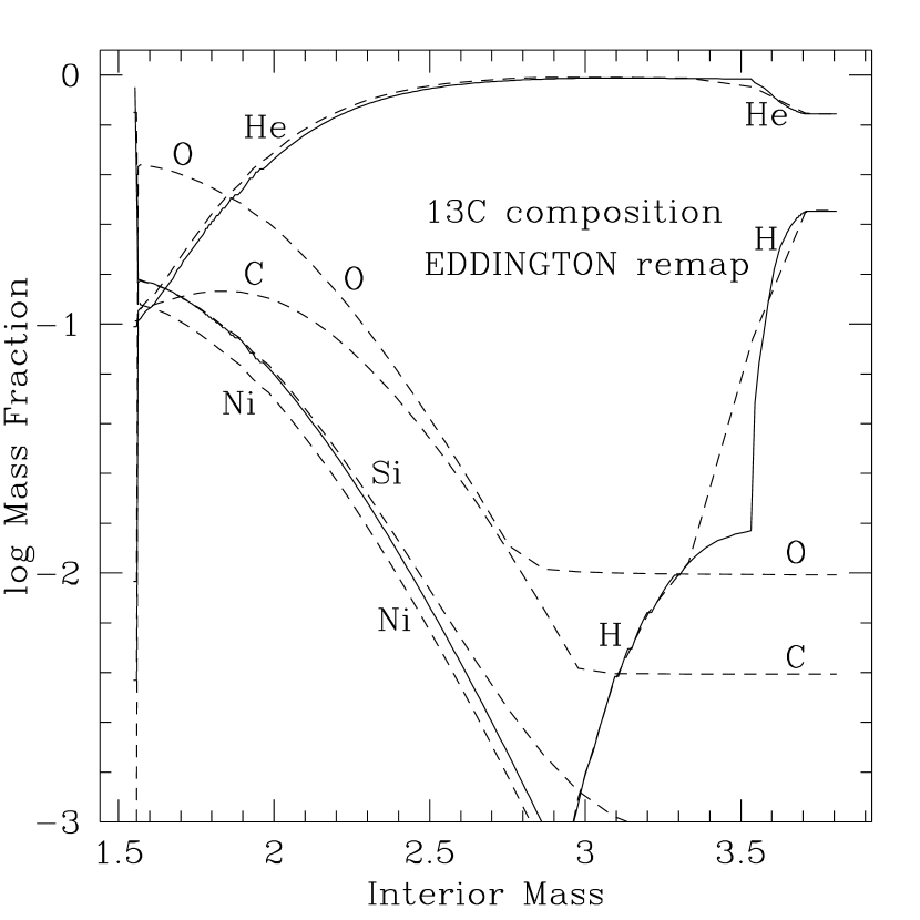
Figure 6: The composition in Model 13C as remapped by EDDINGTON (dashed). Solid lines show original H, He and ⁵⁶Ni distribution in 13C

5 THE LIGHT CURVE AT VARIOUS TIMES

5.1 General features of the model light curves

The first runs of STELLA for Model 13C assumed that the line opacity was scattering dominated (some weak absorption was present according to Anderson, 1989) and that the effect of expansion small. The expansion parameter, $t_{s}$, was set to 100 days. The resulting curves for Model 13C1 are the solid lines in Figure7. Dashed lines are the results of EDDINGTON. Observations of Richmond et al. (1994) are shown by crosses. We see that Model 13C1 produces, for this form of opacity, too little luminosity both in comparison with observations and with EDDINGTON. $UBV$ fluxes also indicate that the model is too hot (too bright in $U$). Figure7 gives all values in the frame comoving with the outer radius of the supernova model (below we discuss the transformation to the rest observer frame), but it is already clear that this correction, which is of order $u/c$ for $M_{\rm bol}$, cannot explain such a large discrepancy. The effect of the expansion on opacity is also insufficient (see below).

Figure 7: $M_{\rm bol}$ and $UBV$ for Model 13C1 (with scattering dominating in the opacity). Results of EDDINGTON are shown by dashed lines

The chief difference here is the treatment of the line opacity. In the EDDINGTON calculation, the line opacity was treated as purely absorptive (possible justification for this is discussed below). Near the secondary maximum ($t\simeq 20$ days) the models are already semi-transparent and the emission, which is low for the case of scattering dominated line opacity, can be enhanced by increasing the absorptive opacity (while keeping the total extinction the same). This is a consequence of the Kirchhof’s law, $\bar{\eta}_{\nu}=\chi_{\rm a}b_{\nu}(T)$ for the emission coefficient $\bar{\eta}_{\nu}$ in (5).

In order to maximize the effect we assumed, in calculation 13C2, that all the extinction was purely absorptive. Figure 8 compares directly the two bolometric light curves of 13C1 (scattering) and 13C2 (absorptive). The difference is striking. In the scattering case (dashed line) the brightness at the second peak is half a magnitude fainter. The total opacity (the extinction) was the same in both calculations, and one cannot say that the effective opacity is larger in the case were the line opacity is taken as scattering. Such a result is indicative of the fact that by the time of the second peak, the radiation field is not in the equilibrium radiative diffusion (ERD) regime, where $J_{\nu}\approx B_{\nu}(T)$ and $H_{\nu}\approx-(1/\chi_{\nu})(\partial B_{\nu}\bigl{(}T(r)\bigr{)}/\partial r)$ and $\chi_{\nu}$ is the total opacity. In ERD it makes no difference whether the opacity is absorptive or scattering, but here one can see directly the effect of enhanced volume emission due to the enhanced absorption.

Figure 8: Comparison of $M_{\rm bol}$ for run 13C1 with scattering lines (dashed) and 13C2 with forced absorption (solid)

The assumption of full absorption in the run 13C2 may overestimate the effect, but we shall see that if one assumes the opacity is purely absorptive only in lines, the difference with this maximum absorption case is not large. Lines dominate the total extinction in the case under consideration.

What is the physical justification for ascribing this enhanced absorption to a process that is, microscopically, actually scattering? When a photon Doppler shifts into resonance with a line and is absorbed, the quanta will scatter around in the line until one of three things happens: the photon may escape from the resonance region, in which case we would regard the interaction as a scattering event. The excited state could be depopulated by an electron collision, in which case we would regard the interaction as an absorption event. A third possibility is that the excited state is depopulated radiatively via an alternate channel, and one or more fluorescence photons emitted. This last possibility turns out to be important.

Considering only the upper and lower levels of a transition, the probability that a trapped photon is collisionally depopulated may be written

$$p(\hbox{therm})={C_{ul}\over C_{ul}+A_{ul}\beta_{ul}}\approx$$

$$\approx{N_{e}\over N_{e}+q\beta_{ul}\left({h\nu/1\ \hbox{eV}}\right)^{3}}$$ (16)

where $C_{ul}$ is the downward collision rate, $A_{ul}$ is the spontaneous decay rate, and $\beta_{ul}$ is the Sobolev escape probability, given by $\beta_{ul}=(1-\exp(-\tau_{ul}))/\tau_{ul}$. The last expression on the right is from Anderson (1989) who, by using the Van Regemorter (1962) approximation and oscillator strengths from Kurucz finds that for iron, $q\sim 10^{13}$ to $10^{14}\ \hbox{cm}^{-3}$. In Model 13C at 15 days, $N_{e}\lesssim 10^{11}\ \hbox{cm}^{-3}$. Taking $q=10^{13}\ \hbox{cm}^{-3}$ and $h\nu=6$ eV, we get the result that only lines with

$$\tau_{ul}\gtrsim 2\times 10^{4}\left({10^{11}\ \hbox{cm}^{-3}\over N_{e}}\right)$$ (17)

are likely to experience collisional destruction. Much of the UV line opacity however comes from transitions with $\tau_{ul}\lesssim 1$. One might be tempted to conclude that the line opacity should be treated as scattering. However this analysis neglects another possibility, that of fluorescence. Pinto and Eastman (1997) analyzed the relative probabilities of escape, thermal destruction and fluorescence and found, for similar physical conditions, that fluorescence may be as much as 5 to 10 times more likely than escape. This mechanism allows a short wavelength photon to be split into two or more long wavelength photons which see a smaller opacity and optical depth to the surface. Within the context of LTE, a crude way to take this process into account is by assuming that photons absorbed in line transitions are thermally destroyed. This provides a mechanism for them to be thermally re-radiated at longer wavelengths, but it is only a crude representation of the real physics, which involves simulating the fully non-LTE population kinetics. Nugent et al [1995,1997] treated many lines of Fe II in full non-LTE, but found that, in order to match observations, they had to introduce a large value of the thermalization parameter for other lines in their models. As pointed out above, the ”naive” assumption that lines should be treated as pure scattering seems pretty reasonable if one asks the question, ”given the relevant range of electron densities, what is the probability that collisional deexcitation will thermalize a photon in resonance with a line”. Treating the line opacity as purely absorptive is a crude, zeroth order attempt at accounting for the effect of splitting in an LTE calculation. See also, for example, Höflich (1995), and Li& McCray (1996) on other approaches to the fluorescence effect, and Jefferies (1968) and Canfield (1971) for early attempts to account for it.

Figure 9 gives the resulting light curves for the forced absorption case of Model 13C2. With enhanced absorption, the STELLA results are in much better agreement with those of EDDINGTON, and with the observations of SN 1993J. At this level of accuracy it becomes worthwhile to take into account the corrections for the transformation to the observer frame.

Figure 9: $M_{\rm bol}$ and $UBV$ for the run 13C2 (forced absorption) shown by solid lines. EDDINGTON - dashed lines

5.2 Transforming to the observer frame

EDDINGTON solves for both the comoving frame intensity and the low order angular moments (energy density and flux), at each time step, so it is straightforward to transform the angle dependent specific intensity into the frame of an observer at rest to obtain the observer frame flux. In STELLA however, the specific intensity is not updated at every time step, although the comoving frame energy density and fluxes are. To transform the comoving frame surface flux into the observer frame, one could use the formula proposed by Mihalas & Mihalas (1984, eq. [99.39])

$$F_{\nu}(observer)=F_{\nu}+u(E_{\nu}+P_{\nu})-[\partial(\nu uP_{\nu})/\partial\nu]\;.$$ (18)

However, this formula assumes that the $P_{\nu}$ is smoothly varying with frequency, whereas there are usually large jumps in flux with frequency. Another approach was necessary in STELLA.

To find the observer frame flux, $F^{o}_{\nu_{o}}$, the following procedure is performed: the radially propagating photon received by an observer at rest, at frequency $\nu_{o}$, has the Doppler-shifted frequency $\nu=\nu_{o}(1-u/c)$ in the comoving frame at the outer radius, where $u$ is the speed of the outermost layers. The idea is to assume that the flux for the observer at rest, $F^{o}_{\nu_{o}}$, is close to the comoving flux, $F_{\nu}$. The frequency $\nu$ falls into an interval $(\nu_{j},\nu_{j+1})$ of the frequency grid in the comoving frame. $F^{o}_{\nu_{o}}$ is logarithmically interpolated between the comoving frame fluxes $F_{\nu_{j}}$ and $F_{\nu_{j+1}}$:

$$F^{o}_{\nu_{o}}=C_{F}(\nu_{o})\exp[w\ln F_{\nu_{j}}+(1-w)\ln F_{\nu_{j+1}}]\;.$$ (19)

The weight $w$ is simply the relative distance of the frequency $\nu$ from the grid points on a logarithmic scale: $w=\ln(\nu_{j+1}/\nu)/\ln(\nu_{j+1}/\nu_{j})$, and $C_{F}(\nu_{o})$ is a correction coefficient: it measures how close $F^{o}_{\nu_{o}}$ is to $F_{\nu}$. This correction factor is found from solution of the transport equation for the specific intensity $I_{\nu}(\mu)$, (which we reiterate, is not performed at every time step). The integration yields $I_{\nu}(\mu)$ for a set of angles with cosines $\mu$, which is Lorentz transformed into the observer frame and used to compute the observer frame flux, $\tilde{F}^{o}_{\nu_{o})}$. From $I_{\nu}(\mu)$ a comoving frame flux is also computed, $\tilde{F}_{\nu}$. One then writes

$$\tilde{F}^{o}_{\nu_{o}}=C_{F}(\nu_{o})\exp[w\ln\tilde{F}_{\nu_{j}}+(1-w)\ln\tilde{F}_{\nu_{j+1}}]\;,$$ (20)

which, since $\tilde{F}^{o}_{\nu_{o}}$ and $\tilde{F}_{\nu}$ are known, gives the correction coefficient $C_{F}(\nu_{o})$. We find that $C_{F}(\nu_{o})$ changes only slowly between time steps, so we get the observed fluxes $F_{\nu_{o}}$ using values of $C_{F}(\nu_{o})$ determined at the last time step at which the specific intensity and Eddington factors were updated. To preserve global energy balance, the monochromatic fluxes are normalized to the observer frame bolometric flux, $F^{o}$, which is easily obtained from frequency integrated quantities in the comoving frame using

$$F^{o}=F+u(E+P)\ ,$$ (21)

which may be obtained by integrating equation 18 over all $\nu$.

One can compare the result of the transformation for Model 13C2 in Figure 10 with the same model in the comoving frame in Figure 9. The effect of the transformation is larger for the broad band fluxes than for $M_{\rm bol}$, especially for $U$, since now at a given wavelength one observes photons which were at shorter wavelengths in the comoving frame, and in the blue part of the spectrum the continuum flux $\lambda$ variation is larger, approximately obeying the Wien’s law.

Figure 10: The same as in Fig 9 but STELLA results (solid lines) are now transformed to the observer frame

In both cases we see that the minimum in $M_{\rm bol}$ for $t\sim 7-10$ days produced by STELLA is more pronounced than that of EDDINGTON. Tests showed that this result is very sensitive to the zoning of the model and abundance distribution (compare Figs. 2 and 6), so it is more instructive to compare the results of the two codes for the exactly the same zoning.

5.3 The influence of physical assumptions on the light curves

Runs 13C4 – 13C8 in Table 1 used exactly the same zoning and chemical composition as was used by EDDINGTON. The results are given in Figures 11 – 15.

Figure 11: $M_{\rm bol}$ and $UBV$ for the run 13C4 of STELLA (scattering dominated line opacity and the same zoning as used by EDDINGTON) shown by solid lines. EDDINGTON - dashed lines

Figure 12: $M_{\rm bol}$ and $UBV$ for the run 13C5 (absorption dominated lines) shown by solid lines. EDDINGTON - dashed lines

Figure 13: $M_{\rm bol}$ and $UBV$ for the run 13C6 (forced absorption for all types of extinction) shown by solid lines. EDDINGTON - dashed lines

Figure 14: $M_{\rm bol}$ and $UBV$ for the run 13C7 (forced absorption as in Figure 13 but now with full expansion effect according to Eq.15) shown by solid lines. EDDINGTON - dashed lines

Figure 15: $M_{\rm bol}$ and $UBV$ for the run 13C8 (absorption dominated lines as in Figure 12, but now with full expansion effect according to equation 15) shown by solid lines. EDDINGTON - dashed lines

The run 13C4 with scattering dominated lines is similar to 13C1, but now all fluxes are given in the observer’s frame, and are found to be too low in comparison with observations.

The runs 13C5 (absorption in lines) and 13C6 (forced absorption for all processes) are very similar. The bolometric light curve is already very close to the results of EDDINGTON, but the $U$ flux is higher. The explanation of this last discrepancy is simple: the runs 13C4 – 13C6 assumed virtually no expansion effect in the line opacity, the parameter $t_{s}=100$ days, and the $U$ band is especially sensitive to the expansion effect of ultraviolet forest of metal lines. So for the runs 13C7 and 13C8 we included the full expansion effect according to the expression (15) and using the following interpolation algorithm: for five values of the velocity gradient, measured as $1/t_{s}$,

$$t_{s}=1\quad 3.16\quad 10\quad 31.6\quad 100\quad{\rm days}\;,$$ (22)

the opacity for each mass zone was saved in tables. During the runs 13C7 and 13C8 we have used the logarithmic interpolation of those opacity tables for current value of the time after explosion $t$ between the corresponding tabulated values of $t_{s}$.

The effect of expansion opacity brings the bolometric light curves very close to the EDDINGTON’s. A small deviation on the tail is completely explained by a slight difference of the gamma-ray deposition routines. We compare the energy deposited by gamma-rays into the matter in the two codes in Figure 16, and one can see that both codes do the tail of the bolometric light curve consistently.

Figure 16: Logarithm of gamma-ray deposition luminosity, L_⊙, in Models 13C4 - 13C8. Solid STELLA, dashed EDDINGTON

The effect of expansion is especially strong in the $U$ band, and the best agreement of two codes is reached, as anticipated, in the run 13C8 where all physics in STELLA follows the physical input of EDDINGTON most closely.

In the test run 13C2s we also checked the effect of a crude frequency discretization (maximum 20 frequency bins used instead of 100 bins in the standard STELLA runs). We found that $M_{\rm bol}$ is reproduced quite well even with this crude frequency grid, but the $UBV$ fluxes are much less reliable. So full hydrodynamics runs of STELLA with a small number of frequency bins can be used for fast preliminary calculations of bolometric light curves, but a detailed comparison with the broad band photometry requires a reasonably large number of frequency bins.

5.4 Shock break-out

Given the good agreement of the STELLA results both with hydrodynamics of KEPLER and the radiative transfer of EDDINGTON, one trusts that reliable results might be obtained for the continuum spectra of SN 1993J near shock break-out, a time when neither of the two earlier codes could operate accurately. For SN 1993J the problem may be more complicated since the progenitor was distorted by a companion (Woosley et al. 1994), Still the results should still be approximately correct.

Figure 17 gives the mean intensity distribution found by STELLA inside the star just prior to shock break-out. In the intermediate layers the intensity departs strongly from a blackbody since in the extreme ultraviolet the radiation from the deep layers already heated by the shock wave becomes visible. This complicated behavior would be poorly represented in a hydro code that employed only one energy group.

Figure 17: Mean comoving-frame intensity $J_{\nu}$ (in arbitrary units) in all mass zones just prior to shock breakout in the run 13C1. The uppermost curves correspond to the innermost layers and the lowest curve to the spectrum on the surface of the star.

Comparing the parameters near the first maximum found by KEPLER (Model 13B, Fig.16 of Woosley et al., 1994) and STELLA, we find that KEPLER calculates a maximum luminosity $L=4\times 10^{44}$ erg/s, corresponding to $M_{\rm bol}=-22.8$ while STELLA finds $M_{\rm bol}=-23.34$ (13C2) and -23.50 (13C1) (in the comoving frame). KEPLER gives a maximum $T_{\rm eff}$ at 22000 sec of $\sim 130\times 10^{3}$ K and STELLA, $156.3\times 10^{3}$ K and $155.3\times 10^{3}$ K respectively both at 0.267 d = 23070 sec. Curves of $M_{\rm bol}(t)$ are given in Figure18 and of $T_{\rm eff}$ in Figure19.

Figure 18: Early bolometric light curve in the frame comoving with the outer radius of supernova. Dashed for Model 13C1 (scattering), solid for Model 13C2 (absorption). Dots for the latter model in the obsever frame

Figure 19: Early $T_{\rm eff}$. Dashed for Model 13C1 (scattering), solid for Model 13C2 (absorption).

It is not trivial to define an effective temperature for a multi-frequency result. STELLA uses the following algorithm for finding $T_{\rm eff}$. At each time step and for any frequency we know the flux $H_{\nu}$ and the Eddington factor, $h_{\nu}=H_{\nu}/J_{\nu}$, for the outer boundary. If we assume, that the intensity $I_{\nu}$ is constant within a certain solid angle and zero outside (a hot spot of uniform brightness), then $I_{\nu}=J_{\nu}/(1-h_{\nu})$. For a blackbody with $T_{\rm eff}$,

$$aT_{\rm eff}^{4}=\sum_{\nu}B_{\nu}dw_{\nu}$$ (23)

If we replace $B_{\nu}$ by the actual $I_{\nu}$ we find

$$aT_{\rm eff}^{4}=\sum_{\nu}J_{\nu}dw_{\nu}/(1-h_{\nu})$$ (24)

With this definition we first define “the last scattering radius”, and then the $T_{\rm eff}$ from $L=\sigma T_{\rm eff}^{4}R_{\rm ph}^{2}$ relation. This $T_{\rm eff}$ it is not necessarily associated with the temperature of any physical layer. As one can see in Figure 19 this $T_{\rm eff}$ is practically equal in models 13C1 and 13C2, that is for scattering and absorption dominated opacity respectively. In the case of absorption this $T_{\rm eff}$ is equal (to accuracy of order of one percent) to the matter temperature at optical depth 2/3, but in the case of scattering the matter at this depth is hotter by 20 – 30 percent.

Figure 20 gives the spectral luminosity for Models 13C1 and 13C2 around the first maximum at t=0.27 day. In the case of absorption the spectrum is nearly a blackbody with a maximum $\lambda\simeq 200\AA$. This gives a temperature $T_{\rm Wien}\simeq 1.5\times 10^{5}$ K from the Wien displacement law. So in this case our $T_{\rm eff}$ coincides with color and brightness temperatures over a large part of the spectrum. A different result holds for the scattering case, Model 13C1. Now the spectrum deviates strongly from a blackbody and the maximum at $\lambda\simeq 60\AA$ gives $T_{\rm Wien}\simeq 4.8\times 10^{5}$, three times $T_{\rm eff}$. In the range of spectrum corresponding to visual light both brightness and color temperatures are lower than $T_{\rm eff}$ in the scattering model. For example, $U-B=-1.2$ for 13C1 and $U-B=-1.3$ for 13C2 near the first maximum light. Thus in visual light the scattering model might be classified by observations as the cooler one which is opposite to reality. This is simply the effect of dilution of a very hot radiation born far below optical depth 2/3.

When discussing the second maximum of the light curve, we found that Model 13C2 (fully absorptive opacity) was in better agreement both with observations and with NLTE theory. At the second maximum the actual opacity is dominated by lines and photoionization so Model 13C3 (absorptive lines, but realistic electron scattering) is practically the same as 13C2 at that epoch. Here at the first maximum light the situation is different. The opacity is overwhelmingly dominated by electron scattering and now Model 13C1 is more physical. For the earliest epoch 13C3 is almost the same as 13C1, so the results at shock breakout are not sensitive to the treatment of lines as absorptive or scattering.

Figure 20: Comoving luminosity at first maximum light for t=0.27 d. Dashed for Model 13C1 (scattering), solid for Model 13C2 (absorption).

Observers often estimate the photospheric temperature from blackbody spectral fits, and this color temperature can be either higher or lower than $T_{\rm eff}$ (Eastman, Schmidt, & Kirschner 1996). If the blackbody fit is good near the wavelength of peak emission, then the color temperature is closer to the temperature at the depth of thermalization, but in this case $R_{\rm ph}$ is neither the surface of last scattering, nor the thermalization radius (for hot, scattering dominated envelopes, it is much too small), so one must exercise caution when comparing the theoretical predictions with the ‘photospheric’ parameters found by observers in these situations (see Blinnikov & Kozyreva 1998 for the analysis of the fits to early spectra of SN 1993J).

At late time $T_{\rm eff}$, as defined here, is much too low in comparison to values given by observers, e.g. for $t=100$ days in the model 13C8 this definition gives $T_{\rm eff}\approx 2000$ K, while Richmond et al. (1994) give blackbody $T\approx 5900$ K. $T_{\rm eff}$ here is neither the color temperature, nor the matter temperature at $\tau=2/3$ (for late times the total optical depth is too low and the definition of equation [24] looses its basic foundation: there is no “last scattering radius”, since only a small fraction of photons experience a scattering). We note, however, that $T_{\rm eff}$ is not a particularly convenient parameter for comparison with observations.

Figs 21 and 22 display the outgoing spectrum for selected moments of time near the first maximum.

Figure 21: Emerging spectral luminosity at the shock breakout in the observer frame for the run 13C1. The curves are labeled by the retarded time in days.

Figure 22: The same as in Figure 21 but after the shock breakout.

Light curves for the case of pure scattering in lines (Model 13C1) and the case of pure absorption in lines (Model 13C3) agree very well at early times. This is because the opacity at these epochs is dominated by electron scattering.

6 CONCLUSIONS

We have calculated light curves for Model 13C of Woosley et al (1994) for SN 1993J using two treatments of radiation transport, EDDINGTON (Eastman and Pinto 1993) and STELLA. The explosion was calculated with both STELLA and KEPLER. Good agreement was found between the two codes for asymptotic profiles of density and velocity. We also found good agreement between STELLA and EDDINGTON (and observations) for the light curves and photometry, $M_{\rm bol}$ and $UBV$.

For times later than a few days after the second peak, the behavior of SN 1993J’s $U$ band light curve is in marked disagreement with either of the two predicted $U$ light curves. A large disagreement is possible here because only a small fraction of the light comes out in the ultraviolet. The ultraviolet flux comes from a thin surface layer where the heating and cooling are dominated by non-LTE processes not included in the present calculation.

We have found that near the epoch of the second maximum of our light curves additional cooling is necessary for better agreement with observations and that the effects of expansion line opacity are very important for the $U$ band. EDDINGTON results and the $UBV$ fluxes of STELLA sometime deviate substantially, especially at very late times, i.e., on the tail of the light curve, but all those differences are within reasonable limits given the uncertainty in opacity data and non-equilibrium physics of late stages of light curves.

At shock breakout the uncertainties in opacity are not so important, so one may hope to obtain even better predictions for an ultraviolet flash at the shock breakout with a code like STELLA (where all important effects in radiative transfer like aberration, Doppler shift and time retardation are taken into account and are coupled to hydrodynamics). At these stages the uncertainty of predictions must lie in the uncertainty of the structure of the outermost layers of a presupernova, in the presence of a superwind, or in effects of asphericity.

Having calibrated the radiation hydro package STELLA both against observations of SN 1993J and a more detailed numerical treatment of just the radiation transport, we are now prepared to embark on modeling the light curves of other Type II and eventually, Type I supernovae. New predictions for the ultraviolet luminosity of SN 1993J during its earliest moments are given in Figures 21 – 22

Appendix A Artificial radiative diffusion

The system (5) – (6) is of a hyperbolic type. The difference scheme used for its numerical solution with fluxes on the mesh cell boundaries and energies in the cell centers has second order accuracy on a uniform grid and a low diffusivity, but does not take into account the hyperbolic nature of equations. For hyperbolic systems other schemes, those which make use of characteristic-ray solutions of equations, are more natural. But it is their common property that when they are very stable, they are highly diffusive. As an example let us consider the simplest equation

$$y_{t}+cy_{x}=0\;,$$ (A1)

where subscripts denote respective partial derivatives. The characteristic-ray of (A1) is $x-ct={\rm const}$, so the solution is $y=f(x-ct)$. Let $x_{0}$, $x_{1}=x_{0}+\Delta x$, and $x_{2}=x_{0}+2\Delta x$ be the nodes of a uniform $x$-mesh. Then the simplest first-order upwind approximation for $y_{x}$ at the point $x_{1}$ is the donor-cell one,

$$y_{x}=(y_{1}-y_{0})/\Delta x\;,$$ (A2)

and this approximation gives good stable results in many practical situation. Yet the more accurate, second order approximation to $y_{x}$ at $x_{1}$,

$$y_{x}=(y_{2}-y_{0})/(2\Delta x)\;,$$ (A3)

shows that in fact the donor-cell prescription (A2) approximates to the second order in $\Delta x$ not the equation (A1), but

$$y_{t}+cy_{x}=c\Delta xy_{xx}\;,$$ (A4)

that is a strong diffusion with the diffusivity $c\Delta x$. The progress of numerical schemes in gas dynamics, e.g. the development of Godunov-type approach, has successfully overcome the excessive diffusivity, but some scheme diffusion is always needed for the stability of calculations.

We argue that in our case the diffusion is not only needed for stability - it has a direct relevance to the description of the correct propagation of radiative flux and energy for flashing surfaces. Let us consider a simple problem (cf. Imshennik, Nadyozhin & Utrobin 1981 where a more difficult problem is solved). Let a horizontal plane surface $S$ be dark for time $t<0$ and bright with intensity $I_{\nu}$ constant in time and uniform in all directions for $t\geq 0$. If an observer is above the plane $S$ at distance $z$ and there is pure vacuum between the plane and the observer, then at the moment $t=z/c$ he sees not the whole bright surface $S$ but only a bright point directly under him. For $t>z/c$ the point becomes a growing bright spot, and the cosine of the angle to the edge of the spot relative the vertical direction is just $\mu_{\rm s}=z/ct$. Now we have for the angular moments of intensity:

$$J_{\nu}={1\over 2}\int_{z/ct}^{1}I_{\nu}d\mu={I_{\nu}\over 2}\biggl{(}1-{z\over ct}\biggr{)}$$ (A5)

$$H_{\nu}={1\over 2}\int_{z/ct}^{1}I_{\nu}\mu d\mu={I_{\nu}\over 4}\biggl{(}1-{z^{2}\over c^{2}t^{2}}\biggr{)}$$ (A6)

$$K_{\nu}={1\over 2}\int_{z/ct}^{1}I_{\nu}\mu^{2}d\mu={I_{\nu}\over 6}\biggl{(}1-{z^{3}\over c^{3}t^{3}}\biggr{)}$$ (A7)

We see that the flux and energy of radiation grow very smoothly, they are smeared by the retardation, whereas the Eddington factor $f_{\rm E}$ jumps from initial $1/3$ (for initial low but non-zero brightness) to $1$ at the moment $t=z/c$ and later it relaxes back to $1/3$ according to the relation

$$f_{\rm E}={1\over 3}\biggl{(}1+{z\over ct}+{z^{2}\over c^{2}t^{2}}\biggr{)}$$ (A8)

To calculate the $f_{\rm E}$ jump very accurately is not an easy task, but our goal is not $f_{\rm E}$ but the flux and the energy and they behave quite smoothly.

That is, contrary to gas dynamics, with its shock waves, instantaneous flashes on a star surface do not produce (in exact solutions) any jumps in $J$ or $H$, due to time retardation. Thus an additional diffusivity in this case does not destroy the correct solution. The explicit form of the stabilizer is presented by the following expression

$$\dot{\cal H}_{\nu_{\rm diff}}=cR_{\rm vis}{{\cal H_{\nu}}_{0}r^{2}_{0}-2{\cal H_{\nu}}_{1}r^{2}_{1}+{\cal H_{\nu}}_{2}r^{2}_{2}\over 2\Delta r\,r^{2}_{1}}\;.$$ (A9)

The subscripts $0$, $1$, $2$ denote here the numbers of subsequent radial zones. The coefficient $R_{\rm vis}$, the ‘artificial radiative viscosity’, is of order unity in the transparent zones (then the diffusivity of the donor cell scheme (A4) is reproduced there) and should be put equal to zero for large optical depth. As our experiments show, the exact way of doing this is not decisive, since the stabilizer (A9) is important only at transient stages of fast variations of flux and is zero for cases when the luminosity does not depend on radius. Moreover, there is no artificial viscosity added to the zeroth moment (monochromatic radiative energy) equation (5) which actually governs the time behavior of the solution.

Appendix B Acceleration of mixing

There is some ambiguity in the treatment of large density contrasts developing in the one-dimensional modeling of shock propagation in radiating fluids (cf. Falk & Arnett 1977). After experimenting with various prescriptions, the following expression for $a_{\rm mix}$ at point 1 (for mesh points numbered 0, 1, 2) was found to produce satisfactory results:

$$a_{\rm mix}=R_{\rm cut}(\tau_{2})u_{2}\min(0,\hbox{div}\,u|_{3/2})-$$

$$-R_{\rm cut}(\tau_{1})u_{0}\min(0,\hbox{div}\,u|_{1/2})\;.$$ (B1)

Here the cutting factor $R_{\rm cut}$ provides a normalization of the effect of the artificial acceleration, is equal to zero in the outermost zone, and kills $a_{\rm mix}$ at optical depths $\tau>1$. The expression (B1) looks very much like a gradient of a viscous pressure, but it is constructed in such a way, that in effect it does not change the kinetic energy integral. One can easily verify this using the relation $2u_{i}a_{i}=2u_{i}\dot{u}_{i}=du_{i}^{2}/dt$ and the expression (B1) for $a_{i}$ and summing over all zone numbers $i$. Thus $a_{\rm mix}$ only redistributes the kinetic energy between neighboring mass shells, where there is a strong compression, i.e. $\hbox{div}u$ is negative, and, contrary to the artificial viscosity $q$, one may not include any effect associated with $a_{\rm mix}$ into the energy equation.

References

- (1)
- (2) Ambwani, K., & Sutherland, P. G. 1988, ApJ, 325, 820
- (3) Anderson, L. S. 1989, ApJ, 339, 558
- (4) Arnett, W. D. 1980, ApJ 237, 541
- (5) Arnett, W. D. 1982, ApJ 253, 785
- (6) Baron, E., Hauschildt, P. H., & Mezzacappa, A. 1996a, MNRAS, 278, 763
- (7) Baron, E., Hauschildt, P. H., Nugent, P., & Branch, D. 1996b, MNRAS, 283, 297
- (8) Bartunov, O. S., Blinnikov, S. I., Pavlyuk, N. N., & Tsvetkov, D. Yu. 1994, A&A, 281, L53
- (9)
- (10) Blinnikov, S. I. 1996, Pis’ma v AZh, 22, 92 (Astron. Letters. J. Astron. Space Sci. 22, 79)
- (11)
- (12) Blinnikov, S. I. 1997, in the proceedings of NATO ASI ‘Thermonuclear Supernovae’ P. Ruiz-Lapuente et al. (eds.), Kluwer Acad. Pub., p. 589
- (13)
- (14) Blinnikov, S. I., & Bartunov, O. S. 1993, A&A, 273, 106
- (15)
- (16) Blinnikov, S. I., & Dunina-Barkovskaya, N. V. 1994, MNRAS, 266, 289
- (17)
- (18) Blinnikov, S. I., Nadyozhin, D. K. & Bartunov, O. S. 1991, in High-Energy Astrophysics, ed. W. H. G. Lewin, G. W. Clark, R. A. Sunyaev (Washington: National Academy Press), 39
- (19)
- (20) Blinnikov, S. I., & Panov, I. V. 1996, Pis’ma v AZh, 22, 45 (Astron. Letters. J. Astron. Space Sci. 22, 39)
- (21)
- (22) Blinnikov, S. I., & Kozyreva, A. V. 1998, in preparation
- (23) Canfield, R. C. 1971, A&A, 10, 54
- (24)
- (25) Carbon, D. 1979, Ann Rev A&A, 17, 513
- (26)
- (27) Castor, J.I. 1972, ApJ, 178, 779
- (28)
- (29) Castor, J. I., Abbott, D. C., & Klein, R. I. 1975, ApJ, 195, 157
- (30)
- (31) Chetverushkin, V. P. 1985, Matematicheskoe modelirovanie zadach dinamiki izluchayuschego gaza (Moskva: Nauka) - Mathematical modeling of the radiating gas dynamics problems
- (32)
- (33) Eastman, R. G., & Kirshner, R. P. 1989, ApJ, 347, 771
- (34)
- (35) Eastman, R. G., & Pinto, P. A. 1993, ApJ, 412, 731
- (36) Eastman, R. G., Schmidt B. P. & Kirshner, R. 1996, ApJ, 466, 911
- (37) Eastman, R. G., & Woosley, S. E. 1997, ApJ, in preparation
- (38)
- (39) Ensman, L., 1991, Dissertation, University of California, Santa Cruz
- (40)
- (41) Ensman, L., & Burrows, A. 1992, ApJ, 393, 742
- (42)
- (43) Falk, S. W., & Arnett, W. D. 1977, ApJ Suppl., 33, 515
- (44)
- (45) Gehmeyr, M. & Mihalas, D. 1994, Physica D, 72, 320
- (46)
- (47) Goldin, V. Ya. 1964, Zh. Vychislit. Mat. i Mat. Fiz. 4, 1078
- (48)
- (49) Grasberg, E. K., Imshennik, V. S., & Nadyozhin, D. K. 1971, Ap&SS, 10, 28
- (50)
- (51) Herzig, K., El Eid, M. F., Fricke, K. J., & Langer, N. 1990, A&A, 233, 462
- (52) Höflich, P. 1990, Dr. Rer. nat. habil., Ludwig-Maximilians-Universität, Munich.
- (53)
- (54) Höflich, P. 1995, ApJ, 443, 89
- (55)
- (56) Höflich, P., Müller, E., & Khokhlov, A. 1993, A&A, 268, 570
- (57)
- (58) Imshennik, V. S., & Morozov, Yu. I. 1981, Radiatsionnaja relativistskaja gasodinamika vysokotemperaturnyh javlenij, (Moskva: Atomizdat) – Radiation relativistic gasdynamics of high-temperature phenomena
- (59)
- (60) Imshennik, V. S., Nadyozhin, D. K. & Utrobin, V. P. 1981, Ap&SS, 78, 105
- (61)
- (62) Iwamoto, K.; Young, T. R., Nakasato, N., Shigeyama, T., Nomoto, K., Hachisu, I., Saio, H. ApJ 477, 865
- (63)
- (64) Jefferies J. T. 1968, Spectral Line Formation, Blaisdell Pub. Co., Waltham
- (65)
- (66) Karp, A. H. 1980, J. Quant. Spectrosc. Radiat. Transfer, 23, 285
- (67)
- (68) Karp, A. H., Lasher, G., Chan, K. L., & Salpeter, E. E. 1977, ApJ, 214, 161
- (69)
- (70) Kurucz, R. L. 1991, in Stellar Atmospheres: Beyond Classical Models, eds. L. Crivellari, I. Hubeny, & D. G. Hummer (Kluwer:Dordrecht) 441
- (71)
- (72) Li, H. & McCray 1996, ApJ, 456, 370
- (73)
- (74) Lindquist, R. 1966, Ann. Phys., 37, 487
- (75)
- (76) Litvinova, I. Yu., & Nadyozhin, D. K. 1985, Pis’ma v AZh, 11, 351 (Sov. Astron. Lett., 11, 145)
- (77)
- (78) Lucy, L. 1971, ApJ, 163, 95
- (79)
- (80) Lucy, L. 1991, ApJ, 383, 308
- (81)
- (82) Mair, G., Hillebrandt, W., Höflich, P. & Dorfi, A. 1992, A&A 266, 266
- (83) Mihalas, D. 1978, Stellar Atmospheres (San Francisco: Freeman)
- (84)
- (85) Mihalas, D., & Mihalas, B. W. 1984, Foundations of Radiation Hydrodynamics (New York & Oxford: Oxford University Press)
- (86)
- (87) Nadyozhin, D. K., & Razinkova, T. L. 1986, Nauchnye informatsii, 61, 29
- (88) Nugent P., Baron, E., Hauschildt, P. H., & Branch, D. 1995 ApJ 441, L33
- (89) Nugent, P., Baron, E., Branch, D., Fisher, A., & Hauschildt, P. H. 1997 ApJ, 485, 812
- (90) Oran, E.-S., Boris, J. P. 1987, Numerical Simulation of Reactive Flow, Elsevier, N.Y., Amsterdam, London
- (91) Østerby, O., & Zlatev, Z. 1983, Direct Methods for Sparse Matrices. Lecture Notes in Computer Science, Vol. 157, Springer, Berlin-Heidelberg-New York-Tokyo
- (92)
- (93) Peytremann, E. 1974, A&A. 33, 203
- (94)
- (95) Pinto, P. A. & Eastman, R. G. 1997 in preparation.
- (96)
- (97) Richmond, M. W., Treffers, R. R., Filippenko, A. V., Paik, Y., Leibundgut, B., Schulman, E., & Cox, C. V. 1994, AJ, 107, 1022
- (98) Shigeyama, T., Suzuki, T., Kumagai, S., Nomoto, K., Saio, H. & Yamaoka, H. 1994, ApJ, 420, 341
- (99) Sobolev, V. V. 1947, Dvizhuschiesja obolochki zvezd (Leningrad) – Moving envelopes of stars
- (100)
- (101) Swartz, D. A. 1989 PhD Thesis, The University of Texas, Austin
- (102)
- (103) Utrobin, V. P. 1978 Ap&SS, 55, 441
- (104) Utrobin, V. P. 1996, A&A, 306, 219
- (105)
- (106) Van Regemorter, H. 1962, ApJ, 136, 906
- (107) Verner, D. A., & Yakovlev, D. G. 1995, A&A Suppl. 109, 125
- (108)
- (109) Wagoner, R. V., Perez, C. A., & Vasu, M. 1991, ApJ, 377, 639
- (110)
- (111) Weaver, T. A., Zimmerman, G. B. & Woosley, S. E. 1978, ApJ 225, 1021
- (112) Woosley, S. E. 1991 in Supernovae. 10th Santa Cruz Workshop in Astr. Ap. ed. S. E. Woosley (N.Y.: Springer) 202
- (113) Woosley, S. E., Pinto, P. A., Martin, P. G., & Weaver, T. A. 1987, ApJ, 318, 664
- (114) Woosley, S. E., Eastman, R. G., Weaver, T. A., & Pinto, P. A. 1994, ApJ, 429, 300
- (115) Young, T., Baron, E.,& Branch, D. 1995, ApJ, 449, L51
- (116) Zhang, X., & Sutherland, P. 1994 ApJ, 422, 719
- (117)