Synthetic Molecular Clouds from Supersonic MHD and Non-LTE Radiative Transfer Calculations

Abstract

The dynamics of molecular clouds is characterized by supersonic random motions in the presence of a magnetic field. We study this situation using numerical solutions of the three–dimensional compressible magneto–hydrodynamic (MHD) equations in a regime of highly supersonic random motions. The non-LTE radiative transfer calculations are performed through the complex density and velocity fields obtained as solutions of the MHD equations, and more than $5\times 10^{5}$ spectra of ¹²CO, ¹³CO and CS are obtained. In this way we build synthetic molecular clouds of 5 pc and 20 pc diameter, evolved for about one dynamical time from their initial configuration. We use a numerical flow without gravity or external forcing. The flow is super–Alfvénic and corresponds to model A of Padoan and Nordlund (1997).

Synthetic data consist of sets of 90$\times$90 synthetic spectra with 60 velocity channels, in five molecular transitions: J=1$\rightarrow$0 and J=2$\rightarrow$1 for ¹²CO and ¹³CO, and J=1$\rightarrow$0 for CS. Though we do not consider the effects of stellar radiation, gravity, or mechanical energy input from discrete sources, our models do contain the basic physics of magneto–fluid dynamics and non LTE radiation transfer and are therefore more realistic than previous calculations. As a result, these synthetic maps and spectra bear a remarkable resemblance to the corresponding observations of real clouds.

1 Introduction

Stars form from the gravitational collapse of cores in molecular clouds. The conditions under which such collapse occurs are poorly understood. Observations show that molecular clouds in which stars form are chaotic in nature. An understanding of the initial conditions that lead to star formation must take into consideration the complex non–linear magneto–hydrodynamic behavior of these clouds. Such studies are essential to an understanding of star formation on large scales; a process that is fundamental to the description of galaxy formation and the conversion of matter into light in the Universe.

Observations have shown that molecular clouds exhibit highly supersonic line-widths and complex internal structure consisting of clumps, sheets, and filaments (cf. Bally et al 1987). The persistence of supersonic motions has led to the postulate that strong magnetic fields threat the clouds and prevent the efficient dissipation of these motions. Therefore, the observed line widths are assumed to be close to the Alfvén speed in the cloud. However, there is little direct observational evidence for pervasive magnetic fields of the required strength. Furthermore, it has been shown that Alfvén waves do not not increase the dissipation time–scale significantly (Zweibel & Josafatsson 1983; Elmegreen 1985; Padoan & Nordlund 1997), which was the original motivation for models of clouds supported by Alfvén waves.

Other workers have proposed that the chaotic structure of molecular clouds and the power law distribution of mass spectra of substructures is an indication of turbulent dynamics. Possible manifestations of turbulent motions are the Larson relations (Larson 1981), the hierarchical structure of the density field (Scalo 1985), the observed intermittency (high velocity tails) in the line profiles (Falgarone & Phillips 1990), and the self–similarity of molecular cloud edges or mass spectra (Falgarone, Phillips & Walker 1991; Elmegreen & Falgarone 1996; Falgarone & Phillips 1996).

Models by Padoan, Jones, and Nordlund (1997a) and Padoan and Nordlund (1997) have shown that supersonic and super–Alfvénic random flow models reproduce many aspects of the observed structure of molecular clouds, such as for example the near–infrared stellar extinction determinations of Lada et al. (1994). Moreover, Padoan and Nordlund (1997) have shown that these models are consistent with the OH Zeeman measurements and constraints. As we show in this paper, these models also result in synthetic molecular cloud spectra and maps that closely resemble real data.

Interpretation of observational data on molecular clouds requires assumptions about the structure of the emitting gas (e.g. Zuckerman & Evans 1974; Leung & Liszt 1976; Baker 1976; Dickman 1978; Kwan & Sanders 1986; Albrecht & Kegel 1987; Tauber & Goldsmith 1990; Tauber, Goldsmith & Dickman 1991; Wolfire, Hollenbach & Tielens 1993; Robert & Pagani 1993; Park & Hong 1995; Park, Hong & Minh 1996; Juvela 1997). In general, the assumptions used by these authors are not consistent with the dynamics of molecular clouds, and are in most cases limited to the statement that molecular clouds are clumpy. Stenholm & Pudritz (1993) and Falgarone et al. (1994) calculated synthetic molecular spectra from fluid models of clouds. Stenholm & Pudritz (1993) used a sticky particles code with an imposed spectrum of Alfvén waves (Carlberg & Pudritz 1990). They calculated line profiles under the simple assumption of LTE. Falgarone et al. (1994) did not solve the radiative transfer problem but calculated density weighted radial velocity profiles on the basis of the results of a turbulence simulation by Porter, Pouquet & Woodward (1994).

A lot of work has been done to understand the clumpiness of molecular clouds, and many observational studies contain lists of molecular clumps, or cores, with their properties (size, mass, velocity dispersion, etc.). These studies have led to the discovery of scaling laws in the ISM, such as the molecular line width-size relation (Larson 1981; Leung, Kutner & Mead 1982; Myers 1983; Quiroga 1983; Sanders, Scoville & Solomon 1985; Crovisier, Dickey & Kazès 1985; Goldsmith & Arquilla 1985; Dame et al. 1986; Falgarone & Pérault 1987; Solomon et al. 1987; Scoville et al. 1987; Leisawitz 1990; Fuller & Myers 1992) and the clump mass distribution (Myers, Linke & Benson 1983; Blitz 1987; Carr 1987; Loren 1989; Dickey & Garwood 1989; Stutzki & Güsten 1990; Lada, Bally & Stark 1991; Nozawa et al. 1991; Langer, Wilson & Anderson 1993; Williams & Blitz 1993).

Theories to explain such laws have been presented for example by Larson (1981), Ferrini, Marchesoni & Vulpiani (1983), Henriksen & Turner (1984), Scalo (1987), Fleck (1988), Myers & Goodman (1988), Mouschovias & Psaltis (1995), Xie (1997), and Fleck (1996). Unfortunately, the results of these investigations may be questioned because only the projected structure of molecular clouds is observed in the molecular emission line maps. There is no way to de project the data since there in no relation between the observed radial velocity and the line–of–sight position of a feature. Furthermore, these scaling laws suffer from serious confusion problems. Operationally, clumps and other structures are identified by drawing closed contours about local maxima in maps and/or in space–space–velocity data cubes. Many such features may consist of chance superpositions of physically unrelated structures. Confusion is severe in crowded environments such as the interiors of giant molecular clouds and in the inner Galaxy (Scalo 1990; Maloney 1990; Issa, MacLaren & Wolfendale 1990; Adler & Roberts 1992).

Since de–projection is not possible, the only way to correctly interpret observational data from molecular clouds is to project realistic theoretical models of their structure and dynamics into the observed data space. Molecular clouds do contain magnetic fields and supersonic motion. Therefore, models of clouds must be based on solution of the equations that describe magneto-hydrodynamic turbulence (e.g. Zweibel 1994). We have produced numerical simulations of supersonic MHD turbulence that are solutions of the compressible 3-D MHD equations in a regime of highly supersonic random motions (Padoan & Nordlund 1997), and subsequently used a non-LTE Monte Carlo radiative-transfer code (Juvela 1997) to produce synthetic spectra of molecular transitions from our MHD data cubes. More than $5\times 10^{5}$ spectra have been computed that may be compared with observational data. In this paper we describe the procedure used to build synthetic molecular clouds and present several results. The MHD flow was computed in a 128³ box with periodic boundary conditions. Radiative transfer calculations slightly degraded the spatial resolution to produce grids of 90$\times$90 spectra each containing 60 velocity channels.

2 The numerical MHD simulations

Padoan & Nordlund (1997) have shown that a supersonic and super-alfvénic random flow is a good model for the dynamics and structure of molecular clouds and is consistent with the estimated magnetic field strengths in cloud cores. In the present work, we use their numerical run called experiment A (i.e., the super-Alfvénic case). In this section we present the MHD equations and the numerical method used for their solution.

2.1 The equations

We solve the compressible MHD equations:

$${\partial\ln\rho\over\partial t}+{\bf v}\cdot\nabla\ln\rho=-\nabla\cdot{\bf v},$$ (1)

$${\partial{{\bf v}}\over\partial t}+{{\bf v}\cdot\nabla{\bf v}}=-{P\over\rho}\nabla\ln P+{1\over\rho}{{\bf j}}\times{{\bf B}}+{\bf f}_{\rm viscous}+{\bf f}_{\rm external},$$ (2)

$${\partial e\over\partial t}+{{\bf v}}\cdot\nabla e=-{P\over\rho}\nabla\cdot{{\bf v}}+Q_{\rm Joule}+Q_{\rm viscous}+Q_{\rm radiative},$$ (3)

$${\partial{{\bf B}}\over\partial t}=\nabla\times({\bf v}\times{\bf B}-\eta\nabla\times{\bf B})$$ (4)

$${\bf j}=\nabla\times{\bf B},$$ (5)

plus numerical diffusion terms, and with periodic boundary conditions. ${\bf v}$ is the velocity, ${\bf B}$ the magnetic field, ${\bf f}_{\rm viscous}$ is the viscous force, ${\bf f}_{\rm external}$ an external force ($=0$ in these particular experiments), and $P=\rho T$ is the pressure at $T\approx$ const.

We use an isothermal equation of state because the heat exchange is so efficient in molecular clouds, that the temperature remains low in most places.

2.2 The code

The code solves the compressible MHD equations on a 3D staggered mesh, with volume centered mass density and thermal energy, face centered velocity and magnetic field components, and edge centered electric currents and electric fields (Nordlund, Stein & Galsgaard 1996).

The original code works with “per-unit-volume” variables; mass density, momenta, and thermal energy per unit volume. In the super-sonic regime relevant in the present application, we found it advantageous to rewrite the code in terms of “per-unit-mass” variables; $\ln\rho$, $u$, and $E=\frac{3}{2}\frac{P}{\rho}$.

We use spatial derivatives accurate to 6th order, interpolation accurate to 5th order, and Hyman’s 3rd order time stepping method (Hyman 1979).

Viscosity and resistivity are minimized using monotonic 3rd order hyper-diffusive fluxes instead of normal diffusive fluxes, and hydrodynamic and magneto-hydrodynamic shocks are captured by adding diffusivities proportional to the negative part of the velocity divergence, and resistivity proportional to the negative part of the cross-field (two-dimensional) velocity divergence. Further details of the numerical methods are given by Nordlund, Galsgaard & Stein (1996) and Nordlund & Galsgaard (1997).

2.3 The Experiment

Our synthetic molecular cloud data cubes are based on a numerical flow with $\beta_{i}=5.3$, where $\beta_{i}$ is the ratio between gas pressure and magnetic pressure at the initial time, $\beta_{i}=(P_{g}/P_{m})_{i}$. The initial density is assumed to be uniform. The initial velocity field is random and purely solenoidal. The probability distribution is Gaussian and consists of only long wavelength modes. In practice, this in done in Fourier space by including random Fourier components with wave-numbers having a modulus $1\leq k\leq 2$. The initial magnetic field is uniform, and is oriented parallel to the $z$ axis, ${\mathbf{B}}=B_{0}{\mathbf{\hat{}}{z}}$. No external forces are applied so the flow decays in time. The magnetic energy is amplified by stretching of field lines and by compression immediately after the beginning of the simulation and the mean value of $\beta$ becomes $<\beta>\approx 1.0$.

The alfvénic Mach number, ${{\cal{M}}_{A}}$ (), is initially ${{\cal{M}}_{A}}\approx 10$, while the ordinary Mach number (i.e., the ratio of the flow rms velocity and the sound velocity) is initially ${\cal{M}}\approx 5$.

Details about the evolution of this flow, and the property of the magnetic field (especially the relationship between volume density and field strength) may be found in Padoan & Nordlund (1997).

3 The Spectrum Calculations

In order to make direct comparisons with observations we have calculated J = 1–0 and J = 2–1 ¹²CO, ¹³CO and J = 1–0 CS spectra from model clouds where the density and velocity fields are taken from the MHD calculations. Since the LTE approximation might cause significant errors in the calculated spectra we solve the non-LTE radiative transfer problem with a Monte Carlo method (Bernes 1979). This way the effects of the velocity field and of the complex density structure are taken into account accurately.

3.1 The Model Clouds

The initial data cube consists of 128³ cells for which the values of density and macroscopic velocity are obtained from the MHD calculations. These values were rescaled as described in section 4, in order to produce the two cloud models, $A_{1}$ and $A_{2}$, summarized in Table 1. The cloud model $A_{1}$ has average gas density of 400 cm^-3 and rms velocity 1.7 km s^-1; model $A_{2}$ density of 100 cm^-3 and rms velocity 3.4 km s^-1. The largest density values are around 1.0$\cdot$10⁵ cm^-3 in both models, and the kinetic temperature is set to 10 K.

In order to speed up the radiative transfer calculations the data was re sampled into smaller data cubes consisting of 90³ cells. New density and velocity values were calculated by linear interpolation of the larger data set. The velocity dispersion between neighboring cells in the original data cube was calculated and used to approximate the turbulent line widths within each cells of the new data cubes. After the thermal line broadening corresponding to the kinetic temperature of 10 K in hydrogen was added to that line width, the mean intrinsic line width was found to be $\sim$0.7 km s^-1. The kinetic temperature and the molecular abundances were kept constant throughout the clouds. The abundances relative to the abundance of H₂ were 5.0$\cdot 10^{-5}$ for CO, 1.0$\cdot 10^{-6}$ for ¹³CO and 5.0$\cdot 10^{-9}$ for CS.

3.2 The radiative transfer calculations

The radiative transfer calculations were carried out with a Monte Carlo program that is well suited for this kind of a study where the cloud contains complex density and velocity fields. With this method, variations in kinetic temperature, molecular abundances, and external radiation fields may be traced explicitly. However, in the present calculations, the temperature and relative abundances are kept constant and no external radiation field is considered, apart from the 2.73 K background radiation.

Our program is a generalization of the one-dimensional Monte Carlo method (Bernes 1979) to three dimensions. The model cloud is divided into cells in which physical properties of the gas are assumed to be constant and in our case the cells are small cubes. There are, however, important differences between our program and the normal Monte Carlo method and it is therefore necessary to explain some principles of the implementation. A detailed description is given elsewhere (Juvela 1997).

In the normal Monte Carlo method the radiation field is simulated with photon packages representing a number of real photons. The packages are sent from random locations in the cloud towards random directions. Each package is followed out from the cloud and interactions between the molecules and the photons contained in the package are counted. When sufficient number of model photons has been simulated this information is used to solve in each cell the number of molecules on different energy levels and the iteration continues with the new level populations.

We have used a modified method in which the radiative transfer is simulated along lines crossing the cloud uniformly. Photon packages containing cosmic microwave background photons are sent into the cloud along these lines. Photons emitted by a cell are added to the incident photons. The photon numbers, in particular the number of photons absorbed within the emitting cell, are calculated explicitly. This is important if some of the cells are optically thick. In that case the normal Monte Carlo method requires generation of a large number of emission events within each of the optically thick cells.

The radiation field was simulated using photon packets containing complete intensity distributions of the simulated lines. The lines were divided into 60 velocity channels that were treated separately in the calculations and for this reason there are no random errors associated with the generation of model photons with random Doppler shifts. The total velocity range included in the calculations was 10 km s^-1 for the model $A_{1}$ and 20 km s^-1 for the model $A_{2}$ and the channel widths were correspondingly 0.17 km s^-1 and 0.33 km s^-1. The channel widths are much smaller than the line widths and less or equal to the smallest intrinsic line widths found in the cells. The chosen velocity discretization is therefore not expected to affect the results of the calculations.

The number of model photons was about 200 000 per iteration. Each model photon contains the intensity distributions of all transitions. Each model photon also represents the emission from all points along a line of sight through the cloud (instead of just from one point). Therefore, the number of model photons can be much less than required by the normal Monte Carlo method and in this case 200 000 model photons are found to give sufficiently accurate results. New level populations are solved in each iteration from the equilibrium equations and convergence was checked by computing the relative changes in the populations of the six lowest energy levels. The iterations stopped when this change, averaged over all cells in the model cloud, was $\sim$1.0$\cdot$10^-3. In some cells the convergence was much worse than the average. These cells, however, have low densities and are therefore not expected to contribute to the spectra. Furthermore, the calculated spectra depend only on populations on the first three excitation levels and these could be more reliably determined than the number of molecules on the sparsely populated upper levels.

The collision coefficients for CO and ¹³CO were taken from Green & Thaddeus (1976) and Green and Chapman (1978). For these molecules six energy levels were included in the calculations, sufficient for excitation temperatures less than 10 K. The CS collision coefficients are from Turner et al. (1992). For CS, the lowest eight energy levels were included to ease the memory requirements. With T_ex=10 K the number of molecules in the level $J$=7 is less than one percent of the number of molecules in the $J$=1 or $J$=2 states. Since levels are sub-thermally populated, the omission of upper energy levels will not affect the results of our calculations.

3.3 The Spectra

The level populations solved with Monte Carlo simulation were used to calculate molecular line spectra along different direction through the cloud. Spectra were computed on a 90$\times$90 grid. Three separate grids of spectra were calculated to correspond to lines of sight perpendicular to the faces of the MHD data cube. Four other grids were calculated along the diagonal directions. In these cases the maps of 90$\times$90 spectra do not extend over the whole projected cloud area. Each spectrum corresponds to the emitted intensity calculated along a particular line of sight through the cloud. These spectra have not been convolved to synthesize a realistic beam. The spectra contain 60 velocity channels as in the Monte Carlo simulation.

For ¹³CO and CS the optical depths of individual cells were small ($\tau\ll 1$). The average optical depth in ¹²CO, however, was about 0.4 per cell and many cells were optically thick. We have tested the effects of degrading the spacing in the final grids from 90³ to 45³ cells. Despite the high optical depth of some cells, this procedure was found to have only a negligible effect on the calculated line intensities. Only small differences could be seen between these two models. The maximum differences in individual velocity channels were only a few percent. Therefore, the difference between discretization into 90³ or 128³ cells is unimportant for the spectrum calculations.

The results were compared with spectra calculated assuming LTE conditions. The comparison showed that in this case the LTE assumption would be unsuitable.

4 Synthetic Molecular Clouds

We have computed 70 grids of 90$\times$90 spectra in the J=1$\rightarrow$0 and J=2$\rightarrow$1 lines of ¹²CO, the J=1$\rightarrow$0 and J=2$\rightarrow$1 ¹³CO, and the J=1$\rightarrow$0 CS. Model $A_{1}$ describes 5 pc clouds while model $A_{2}$ describes 20 pc clouds and Table 1 summarizes their main parameters. For each model we calculate maps corresponding to 7 different lines–of–sight through the 3 projected faces and four projected diagonals of the model data cube.

All clouds have the same mean column density, N(H₂)=6$\times$10²¹ cm^-2, a typical value for observed clouds. Models $A_{1}$ and $A_{2}$ have mean densities $\langle n\rangle=400$ cm^-3 and $\langle n\rangle=100$ cm^-3 respectively. The three-dimensional rms velocity (not the line width), $\sigma_{v}=1.7$ km s^-1 in models $A_{1}$ and 3.4 km s^-1 in models $A_{2}$. These rms velocities produce line widths in agreement with observations. The numerical flow has an rms Mach number $\leq$5. It is easy to re scale the three dimensional velocity fields to other values of the rms Mach number. The density field of a flow with a larger Mach number may also be obtained from statistical properties of random supersonic (and super-Alfvénic) flows found by Nordlund & Padoan (1997), and proven to be in agreement with stellar extinction determinations (Lada et al. 1994) in Padoan, Jones & Nordlund (1997a), and Padoan & Nordlund (1997). The density field is well approximated by a log–normal distribution whose standard deviation is 0.5 times the rms Mach number of the flow. Therefore, if the mean temperature and rms velocity in molecular clouds are known, the statistics of the density field are completely determined. To make the density field consistent with the rescaled velocity field, we scale the logarithm of the density to the correct standard deviation and mean, and then take the exponential. The result is a rescaled density field with the same mean as the original one but with a larger standard deviation, consistent with the velocity field.

5 Results

5.1 Integrated Temperature Maps and Distributions

The complex three-dimensional density field in the numerical flow is illustrated in Fig. 1, using volume projections with different opacity levels. The morphology appears ‘filamentary’ and the density contrast is more than five orders of magnitude. The distribution is Log–Normal as in previous experiments (Nordlund & Padoan 1997; Padoan, Jones & Nordlund 1997). Fig. 1 shows the cumulative volume and mass fractions as functions of density. This allows the present model of the density field to be related to previous clumpy models of molecular clouds used to produce synthetic spectra. For example, in the 5 pc model, 80% of the volume has a density below the mean ($n<$400 cm^-3), and therefore will not give a significant contribution to CO or CS emission. Nevertheless, 30% of the total mass is located in only 1.4% of the volume and is in regions ten times denser than the mean density ($n>$4000 cm^-3). Thus, a significant fraction of the mass but a very small fraction of the volume will contribute to the CO emission. The density distribution in the 20 pc model is even more intermittent because of the larger rms Mach number of the flow. Almost 90% of its volume is below the average density ($n<$100 cm^-3) and about 20% of the mass has $n>$4000 cm^-3. These dense regions occupy only 0.2% of the total volume. It is difficult to compare this complex and intermittent density field to previous models built as ensemble of clumps because in the present case there is a continuous distribution of density values from $n=$0.6 cm^-3 to $n=$10⁵ cm^-3 in the 5 pc model and from $n=$0.01 cm^-3 to $n=$10⁵ cm^-3 in the 20 pc model. Figs. 3-5 show several examples of integrated intensity maps of J=1$\rightarrow$0 transition of ¹²CO, ¹³CO and CS. It is apparent that the CS emission has a lower surface filling factor than the ¹³CO emission and the ¹³CO emission has a lower surface filling than the ¹²CO emission.

The integrated temperature maps are reminiscent of observed clouds. Filaments and clumps are apparent as well as features that look like bubbles and which might be interpreted as shells due to the star formation activity. In our models, this morphology can only be due to the complex system of shocks that develops in the random supersonic flow. It is remarkable that an extremely rich structure is produced even without the effect of gravity, stellar radiation, or stellar outflows. The density contrast is large and comparable to that estimated in dark clouds and the velocity dispersions are realistic.

The probability distribution of the integrated intensity is plotted in Fig. 2 for the j=1$\rightarrow$0 transitions of all three molecules in the 5 pc models. The distributions are obtained from 7 synthetic clouds. While ¹²CO has a rather symmetric (nearly Gaussian) distribution, ¹³CO and CS are characterized by long tails because they sample the column density which is by itself intermittent.

5.2 Spectral Line Profiles

The study of the spectral line profiles is interesting because of previous attempts to use their shape to probe the presence of turbulence in dark clouds. Falgarone & Phillips (1990) studied molecular line profiles of different sources, and found excess emission in the line wings, relative to a Gaussian distribution (see also Blitz, Magnani & Wandel 1988). Miesch & Scalo (1995) looked at the histograms of emission line centroids, and found nearly exponential tails in many cases. Lis et al. (1996) studied the statistics of line centroids and of centroid increments, and found non-Gaussian behavior especially in the histograms of the velocity centroid increments. There is therefore observational evidence of intermittency in the statistics of velocity fields in molecular clouds.

In Fig. 3 we plot the average spectra of the transitions J=1$\rightarrow$0 and J=2$\rightarrow$1, of ¹²CO and ¹³CO. The average is made over seven synthetic maps of the same cloud model, for 5 pc (left), and 20 pc (right), that is to say over 56700 individual spectra. While the ¹³CO spectra are very close to Gaussian, the ¹²CO spectra show saturation and a little bit of self-absorption. All spectra are very smooth and centrally peaked.

Individual spectra are shown in Figs. 4-6. We have plotted only subsets of 20$\times$20 spectra, while the maps contain 90$\times$90 spectra, in order to better visualize the profiles. Individual line profiles often shows multiple velocity components, and this is especially true for ¹²CO. The ¹²CO profiles in high intensity spots are clearly saturated, and this occurs at a radiation temperature of about 7 K. It is difficult to describe the shapes of individual line profiles, because while some are nearly Gaussian, with an excess wing emission (as in the observational analysis by Falgarone & Phillips), some have double or multiple components.

In order to quantitatively illustrate the shape of the individual spectral profiles, we have plotted in Figs. 7-8 the distributions of their first four statistical moments: mean velocity, velocity dispersion, skewness, and kurtosis. The vertical dashed lines in the plots mark the value of the correspondent statistical moment in the averaged spectrum (Fig. 3). The saturation in the ¹²CO spectra manifests itself in lower values of kurtosis relative to the ¹³CO spectra. Both skewness and kurtosis in the 20 pc models (not shown) span a range of values twice as large as in the 5 pc models, although those statistical moments are normalized with the velocity dispersions. The broad distribution of the values of kurtosis around the Gaussian value of 3, is due to the fact that while some lines are just Gaussian plus excess wing emission (kurtosis larger than 3), some have multiple components that tend to flatten the profile (kurtosis less than 3).

5.3 Line-Width Versus Integrated Temperature

Fig. 9 shows the relation between integrated temperature and equivalent width, defined as the integrated temperature divided by the maximum temperature, for ¹³CO, J=1$\rightarrow$0. Heyer, Carpenter & Ladd (1996) have drawn attention to this relation, because it could be used as a way to probe the importance of magnetic fields for the dynamics of molecular clouds. They claim that Alfvén wave models of molecular cloud motions would generate a decreasing line-width with increasing column density. We show here that the numerical super-Alfvénic flow does produce an increasing line-width with increasing integrated temperature, as found in the observations. Plots are obtained as an average on several maps. Plots for single maps are qualitatively the same.

5.4 Line Intensity and Line Width Ratio

The observed line intensity ratios of different CO transitions are found to be approximately constant. Falgarone & Phillips (1996) find $R_{CO}(2-1/1-0)=0.62\pm 0.08$, constant in space, and also across line profiles, in a portion of a cloud edge in the Perseus-Auriga complex. In Fig. 10 the average ¹²CO J=1$\rightarrow$0 (continuous line) and J=2$\rightarrow$1 (dotted line) spectra are plotted for both the 5 pc and the 20 pc models. The J=2$\rightarrow$1 temperature is divided by 0.62, that is the line ratio found by Falgarone & Phillips (1996). Fig. 10 shows that the synthetic spectra from our model clouds have approximately the same intensity ratio has the observed ones. The same is true for the ratios of velocity integrated temperature of single lines–of–sight, shown in Fig. 11. The scatter in the plot is comparable to the observed scatter, although our models produce a ratio that slightly grows with increasing ¹²CO J=1$\rightarrow$0 integrated temperature.

Finally, the ratios of ¹²CO J=2$\rightarrow$1 to ¹³CO J=2$\rightarrow$1 line–widths are plotted in Fig. 12, where the continuous horizontal line is again the value found by Falgarone+91.

6 Discussion

In this work we have illustrated the procedure of obtaining synthetic molecular spectra that may be used to interpret observational data on molecular clouds. The spectrum calculations are based on cloud models that are consistent with the physical conditions in molecular clouds. We have not included gravity in the cloud models, because one of our aims is to show that magneto–hydrodynamics itself, without gravity, can successfully reproduce the structure and kinematics observed in molecular clouds. This is due to the fact that the velocity field is highly supersonic and turbulent. Under these conditions the flow develops a complex system of shocks with very high density contrast, because the cooling time in the molecular gas is so short. Therefore molecular clouds are fragmented primarily by a random system of shocks, and not by gravitational instability, although the formation of protostars inside dense regions of shocked gas is eventually a gravitational collapse. The statistical properties that arise from this scenario of turbulent fragmentation were shown to be in agreement with the statistics of the density field in the dark cloud IC 5146 (Padoan, Jones & Nordlund 1997), studied by Lada et al. (1994) with near-infrared imaging. Padoan & Nordlund (1997) have shown that the same scenario is also consistent with the estimates of magnetic field–strength in molecular clouds. A direct result of this picture is also the successful derivation of the stellar initial mass function (Padoan, Nordlund & Jones 1997b).

There is remarkable qualitative agreement between both the synthetic spectra and the images generated by integrating the spectra over narrow velocity ranges. For example, the CO maps of the Orion region presented by Bally et al. (1987) and by Bally, Langer & Liu (1991) exhibit filamentary morphology and contain voids of various sizes that closely resemble the images presented in this paper. A comparison between the theoretical data cubes and ¹³CO observations of the Perseus molecular cloud obtained with linear resolution comparable to the model calculations shows close agreement in a variety of statistical measures (Padoan et al. 1997).

A detailed comparison of the theory with the observations is now possible and will be presented in future works. The results that have been shown here are certainly reminiscent of the observational data. Some of them are:

• The complex filamentary and clumpy structure of the integrated intensity maps.

• The long tail (intermittency) in the probability distribution of the integrated intensity of ¹³CO and CS.

• The smooth centrally peaked CO average spectra.

• The presence of multiple components and intermittent wings in spectra from individual lines of sight.

• The distributions of statistical moments from individual spectra.

• The relation between integrated intensity and line–width.

• The line intensity and line–width ratios.

All these properties of molecular clouds are nicely reproduced by the numerical flows, even if their initial conditions (eg uniform density and magnetic fields, solenoidal large scale velocity field) are not necessarily a good description of molecular clouds in any phase of their evolution. The success of the numerical models is due to the fact that the system almost immediately loses its memory of the initial conditions. In chaotic dissipative systems such as the present one, the position and velocity of a particle at any given time are, on the one hand, extremely sensitive to the initial conditions, and are therefore individually unpredictable (initial errors grow exponentially with time). On the other hand, such systems also develop some order, or self–organization. The self–organization is apparent in a statistical description (e.g. scaling laws and probability distribution functions). Thus, while a turbulent flow is extremely sensitive to the initial conditions from a mechanic point of view, the initial conditions are almost irrelevant for its statistical description. This is the reason why the numerical modeling is able to predict statistical properties of turbulent flows that are universal, and also measured in molecular clouds. Ironically, the success of the numerical modeling is due to the very large Reynolds number of the motions in molecular clouds, which is usually believed to be the most serious limitation of numerical simulations (eg Scalo 1987).

Model	L (pc)	t (tdyn)	$<n>$ (cm-3)	$\sigma_{v}$ (km/s)	T (K)
$A_{1}$	5.0	1.0	400	1.7	10
$A_{2}$	20.0	1.0	100	3.4	10

Table 1:

Figure 1:

Figure 2:

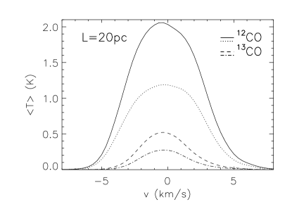
Figure 3:

Figure 4:

Figure 5:

Figure 6:

Figure 7:

Figure 8:

Figure 9:

Figure 10:

Figure 11:

Figure 12: