BLR sizes and the X-ray spectrum in AGN

Abstract

Recent ROSAT studies of narrow-line Seyfert 1 galaxies revealed these objects (with FWHM $H_{\beta}\leq 2000\ km\ s^{-1}$) generally show steeper soft X-ray spectra than broad line Seyfert 1’s and that there are no AGN with broad lines and steep X-ray spectra. We derive a simple theoretical model which explains this observed correlation between the line width and the spectral index for Seyfert 1 galaxies. Assuming the line width is due to gravitational velocity dispersion, it is determined by the radius of the broad line region. Sources with steep X-ray spectra (for a given luminosity) have a stronger ionizing power than flat-spectrum sources with comparable luminosity, which implies that the BLR is formed at relatively larger distances from the central source, and hence has a smaller velocity dispersion and a smaller observed FWHM. We test the model over a hetrogeneous (normal and narrow-line) sample of some 50 AGN finding a good agreement with the data.

1 Introduction

Boller, Brand & Fink 1996 (hereafter BBF96) report the observation with ROSAT of a sample of 49 Narrow-Line Seyfert 1 galaxies (NLS1), finding that NLS1 have generally steeper soft X-ray continua than normal Seyfert 1s. (However, not all NLS1 are remarkably steep). As a result, looking in the FWHM-$\alpha$ plane, there are no AGN with broad lines and steep X-ray spectra.

BBF96 tested NLS1 models assuming they are Seyfert 1 galaxies with pole-on orientation, warm absorption, thick BLR and smaller black hole mass and/or higher accretion rates. The latter showed some promise, but have drawbacks as well, as some NLS1s do not have steep spectra, and on the other hand a smaller black hole mass does not necessarily produce narrower lines (see Sect. 2).

We suggest a simple physical explanation to the observed correlation between the soft X-ray spectral index and the H$\beta$ line width. Assuming the narrower permitted lines reflects a lower Keplerian velocity, we explain the observed correlation by showing that a steeper spectrum has a stronger ionizing power, and hence the BLR form at a relatively larger distance from the central source. (Indeed, the characteristic distance of the BLR estimated by this method, agrees well with the BLR sizes determined by reverberation mapping (Wandel 1996;1997)).

Below we formulate this scanario by combining the assumptions of (1) Keplerian velocity Doppler width for the broad lines, (2) a power-law spectrum of the ionizing continuum luminosity, and (3) characteristic values for the ionization parameter and physical conditions in the BLR.

2 The analytic approach

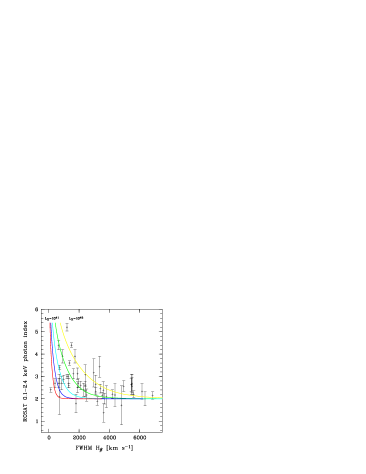
Figure 1: X-ray continuum slope, obtained from a power-law fit, versus FWHM of H$\beta$ for Seyfert 1 galaxies (taken from Walter & Fink 1993) and NLS1 (BBF96). Lines of constant X-ray luminosity are overplotted for the relation given by Eq. 7.

We derive a simple analytic relation between the width of broad emission lines and the continuum slope of the central engine. The observed velocity dispersion is determined by the mass of the black hole and the Broad line region radius. (Note however that the BH mass does not solely determine the BLR velocity; for example, in Bondi accretion we have $\dot{M}\sim R_{a}^{2}$ where $R_{a}\sim GM/kT$ is the accretion radius, so that $\dot{M}\sim M^{2}$. If the efficiency is constant, $L\sim M^{2}$ than $R\sim L^{\frac{1}{2}}\sim M$ so $v\propto M/R\sim const$). Our basic idea is as follows: Sources with steep X-ray spectra (for a given luminosity) have a stronger ionizing power than sources with flat spectra. Since the ionization parameter at the BLR has a characteristic value, a larger ionizing power implies that the BLR is formed at a relatively larger distance from the central source, and hence has a smaller velocity dispersion and a smaller observed FWHM.

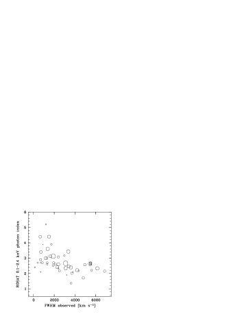
Figure 2: X-ray continuum slope, obtained from a power-law fit, versus FWHM of H$\beta$ for Seyfert 1 galaxies (taken from Walter & Fink 1993) and NLS1 (BBF96).The size of the circles corresponds to the ROSAT luminosity.

We make the following assumptions (rather standard in the literature) :

a. The width of the broad lines is induced by Keplerian motion in the gravitational potential of the central mass. The full width at half maximum is given by:

$$FWHM\approx\left(\frac{GM}{R}\right)^{\frac{1}{2}}$$

where M is the mass of the central black hole and R the radius of the broad line region.

b. The physical conditions in the ionized gas emitting the broad lines are characterized by the ionization parameter U, the ratio of ionizing photons to electrons (cf. Netzer 1990) defined by

$U=Q_{ion}/{4\pi R^{2}}cn_{e}$ where $Q_{ion}=\int_{E_{0}}^{\infty}l(E)\frac{dE}{E}$ is the ionizing photon flux (number of ionizing photons per unit time) l(E) is the monochromatic luminosity of the central source, per unit energy, and $n_{e}$ is the electron density.

The radius of the BLR may be written as

$$R=\left(\frac{L_{ion}}{4\pi c\bar{E}_{ion}Un_{e}}\right)^{1/2}$$

where $L_{ion}=\int_{E_{0}}^{\infty}l(E)dE$ is the ionizing luminosity, and $\bar{E}_{ion}\equiv L_{ion}/Q_{ion}$, is the mean energy of the ionizing photons.

Analyses of the broad emission lines in various AGN indicates that typical values of U for high ionization lines such as H$\beta$ in AGN clouds are 0.1-1 and $n_{e}\sim 10^{10}-10^{11}cm^{-3}$ in the high excitation lines (cf. Rees, Netzer & Ferland 1989) so that $Un\sim 10^{9-11}cm^{-3}$.

$$R\simeq 0.037(n_{10}U\bar{E}_{ion})^{-1/2}L_{i45}^{1/2}pc$$

where $L_{i45}=L_{ion}/10^{45}$erg/s, $n_{10}=n_{e}/10^{10}cm^{-3}$ and $\bar{E}_{ion}$ is in Rydbergs.

This value (cf. Alexander & Netzer 1994), is in agreement with the results from recent reverberation mapping observations (e.g. Clavel et al. 1991, Peterson et al. 1991)

c. Assuming the energy spectrum of the luminosity emerging from the central energy source can be approximated by a power law $l(E)\propto E^{-\alpha}$ we find

$$\bar{E}_{ion}=\frac{\alpha}{\alpha-1}E_{0}.\ \ \ \alpha>1\$$

(Since we are interested only in the ionizing spectrum, between $E_{0}=$1 Rydberg and a few keV, the power law assumption may be a reasonable approximation. Equation 4 holds only for $\alpha>1$, as otherwise $L_{ion}$ and E diverge. This divergence is not physical, as actually the hard X-ray spectrum cuts off at at 50-100 keV).

Combining Eqs. (1), (3) and (4) we have

$$FWHM\approx(1100km/s)\left(\frac{n_{10}U\alpha}{\alpha-1}\right)^{1/4}L_{i45}^{-1/4}M_{7}^{1/2}$$

where $M_{7}=M/10^{7}M_{\odot}$. Since we do not know the ionizing luminosity, we try to express it in terms of the X-ray luminosity and the spectral slope. The observed X-ray luminosity $L_{x}$ is in the ROSAT 0.1-2.4 keV band, while the ionizing luminosity extends to 1Ryd=13.6eV. Assuming the power law spectrum in the ROSAT band may be extrapolated to a lower energy $E_{0}$ we have for the ratio

$${L_{ion}\over L_{x}}=\frac{E_{0}(keV)^{1-\alpha}}{0.1^{1-\alpha}-2.4^{1-\alpha}}\approx(0.14E_{0})^{1-\alpha}$$

where here and below $E_{0}$ without units indicates $E_{0}$ in Rydbergs. Substituting this in Eq. (5) we have

$$FWHM\approx(1100km/s)\left(\frac{n_{10}U\alpha}{\alpha-1}\right)^{1/4}L_{x45}^{-1/4}$$

$$(0.14E_{0})^{(\alpha-1)/4}M_{7}^{1/2}$$

where $L_{x45}=L_{x}/10^{45}$erg/s.

d. We do not know the BH mass of individual objects, but we can use a mass-luminosity relation in a statistical sense, over a large enough sample of AGN, as we did with the ionization parameter above. We assume that the mass is roughly proportional to the luminosity, that is, that the Eddington ratio has a relatively narrow distribution, compared to the range of the luminosity distribution over the sample (e.g. Wandel and Yahil 1985). Defining , $\eta_{x}=L_{x}/L_{Edd}$ where $L_{Edd}=(1.3\ 10^{45}erg/s)M_{7}$, we can then express the central mass in terms of the continuum X-ray luminosity, $M_{7}\approx L_{x45}/\eta_{x}$. Substitutinging this relation in Eq. (6) we have

$$FWHM\approx(1100km/s)\eta_{x}^{-1/2}\left(\frac{n_{10}U\alpha}{\alpha-1}\right)^{1/4}L_{x45}^{1/4}$$

$$(0.14E_{0})^{(\alpha-1)/4}$$

Detemining $E_{0}$ and $\eta_{x}$ will give us a relation between the line width, the spectral index and the X-ray luminosity.

The ratio $L_{x}/L_{Edd}$ is not known, but may be estimated from theoretical and observational arguments. The bolometic $L/L_{Edd}$ is often estimated to be in the range 0.1-1. Observational estimates of $L_{opt}/L_{Edd}$ and $L_{x}/L_{Edd}$ are in the range 0.01-0.1 (e.g. Wandel and Yahil 1985, Wandel & Mushotzky 1986), which may justify a choice of $\eta_{x}=0.1$.

Combining the parameters in Eq. (8) as $P=(n_{10}U)^{1/4}(\eta_{x}/0.1)^{-1/2}$ gives

$$FWHM\approx(5600km/s)1.6^{-\alpha}\left(\frac{E_{0}^{\alpha-1}\alpha}{\alpha-1}\right)^{1/4}L_{x45}^{1/4}P$$

Note that choosing $E_{0}=1$ is equivalent to extrapolating the power law spectrum to 1Ryd, which may overestimate the ionizing luminosity, (especially for large values of $\alpha$) if the spectrum actually flattens at a higher energy. However, because of the weak dependence on $E_{0}$, this effect is small: for example, if $L_{x}=10^{44}erg/s$, $p=1$ and $\alpha=2$ $E_{0}=1Ryd$ gives $FWHM\simeq 1500km/s$, while for $E_{0}=3Ryd$ we get 1800 km/s.

In Fig. 1 we overlay the analytic relation between the FWHM and $\alpha$ with the observed data from Fig. (8) of BBF96 for different values of $L_{x}$. The general shape of the observed distribution and the analytic relation of Eq. (9) are in good agreement. (Note that the convergence of the theoretical curves at a photon index of 2 (corresponding to $\alpha=1$) for large FWHM is not physical; if a high energy cutoff would have been introduced, the curves would extend also to lower values).

3 Predictions and tests of the model

3.1 Line width

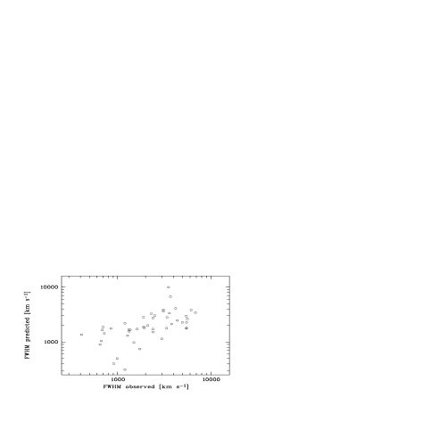
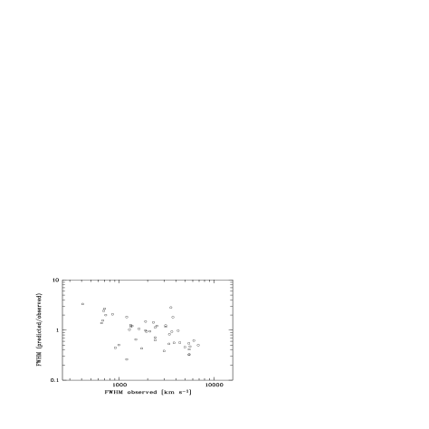
Figure 3: Line width prediction from the model. Left panel (3a): Predicted (from Eq. 9) versus observed FWHM of $H\beta$ for Seyfert 1 galaxies (taken from Walter & Fink 1993) and NLS1 (BBF96). Right panel (3b): Ratio of predicted and observed FWHM versus observed FWHM of $H\beta$.

Using Eq. (8) or (9) we may predict the line width from the observed luminosity and the X-ray continuum slope. Figure 3a shows the predicted line width (model) versus the actually observed one FWHM(observed). Ideally, one would expect all the points to be on the diagonal. However, the scatter in the parameters $\eta_{x}$ and $nU$ (which, in the analytic model we have assumed to have a single value for all objects) and eventualy in the spectral shape of the EUV, can easily explain the scatter in the plot; infact, it is surprising the scatter is not larger than a modest factor of  3.

The ratio between the observed FWHM and the calculated velocity is scattered about unity, and shows no significant dependence on the other observables ($L_{x}$ or $\alpha$), as is expected if the model gives the correct dependence on these observables. The ratio appears to be weakly anticorrelated with the observed FWHM (Fig. 3b), in the sense that very narrow line objects give larger values for the predicted/observed FWHM ratio, and vice verca. However, the correlation coeffient is $\rho=-0.2$ which is insignificant, certainly compared with the $\rho=0.7$ correlation coefficient of the predicted vs. observed FWHM. This indicates that the model probably takes the main effects into account, but there is a systematic residual dependence on the line width.

3.2 Luminosity-dependent $L_{x}/M$

What does this residual dependence tell us? If the basic assumptions made above are correct, the bias has to be sought in the parameters. If, for example, $L_{x}/M$ depended on FWHM, so that it decreased with increasing FWHM, this would reduce the effect, since for objects with larger FWHM Eq. (8) would give larger calculated values and vice versa. One explanation for such a dependence is that objects with narrow lines tend to have a smaller L/M ratio, that is, narrow line objects tend to have relatively smaller mass black holes.

We now present a different, explanation, by showing that such a dependence does indeed follow from the well known phenomenological relation between the optical-UV luminosity ($L_{o}$) and X-ray luminosity in AGN. In transforming the black-hole mass to luminosity we have assumed that the Eddington ratio ($\sim L/M$) is approximately the same for all objects. Since we use the X-ray luminosity, we should actually take into account the ratio $L_{x}/M$, or, $L_{x}/L$. It has been shown that in large samples of AGN $L_{x}\propto L_{o}^{0.75\pm 0.05}$ (Kriss 1988, Mushotzky and Wandel 1989; note however that there is a considerable scatter around this relation). If so, assuming $L_{o}/M\sim$ const. implies (on average)

$$\eta_{x}\propto L_{x}/M\propto L_{o}^{-0.25}\sim L_{x}^{-0.33}.$$

We can plug this into the theoretical relation (Eq. (8) or (9)) to get a phenomenological relation, which gives a modified dependence on $L_{x}$:

$$FWHM\propto L_{x}^{0.25}\eta_{x}^{-1/2}\propto L_{x}^{0.4}.$$

In order to see whether this explains the residual dependence on FWHM (Fig. 3b), we should express the FWHM calculated/observed ratio in terms of FWHM instead of $L_{x}$. Expressing $L_{x}$ in terms of FWHM in Eq. (8) and using Eq. (10) gives $\eta_{x}\propto FWHM^{-0.8}$. Since the values of FWHM calculated in Fig. 3b assume a fixed value for $L_{x}/M$, the calculated/observed FWHM ratio will have a bias of $1/\eta_{x}^{-1/2}\sim FWHM^{-0.4}$ which agrees with the dependence seen in Fig. 3b.

3.3 Luminosities

Figure 4: Luminosity prediction from the model. Upper limit of the predicted ROSAT luminosity vs. observed ROSAT luminosity. We assume an Eddington ratio of $\eta=1$ and a relation between ionizing and ROSAT luminosity of $L_{ion}=7^{\alpha-1}L_{x}$.

Eq. (8) predicts that the X-ray luminosity of individual objects should increase in the direction normal to curves of constant $L_{x}$ in the FWHM-$\alpha$ plane (see Fig. 1). Fig. 2 gives the actual observed ROSAT luminosities (the size of the symbols corresponds to L) indicating a general increase of the observed luminosities as predicted by the analytical relation. Reversing Eq. (9) and using the observed FWHM we have

$$L_{x45}(pred)=7^{\alpha}\left({\alpha-1\over\alpha}\right)E_{0}^{1-\alpha}$$

$$\left({FWHM\over 5600km/s}\right)^{4}(n_{10}U)^{-1}(\eta_{x}/0.1)^{2},$$

so we may calculate a predicted value for the X-ray (ROSAT band) luminosity, assuming e.g. $\eta_{x}=0.1$ (Fig. 4). Comparing this with the observed ROSAT luminosity may be an alternative test of the model. Theoretically, if there were no scatter in the parameters, all objects should lie on the diagonal. The scatter in Fig. 4 appears larger than in Fig. 3a, since the parameters are in the fourth power. We also note that the slope of the best linear regression appears larger than unity, which reflects the residual dependence seen in Fig. 3b. If we assume $\eta_{x}$ does not depend on $L_{x}$, Eqs. (11) and (12) give $L_{x}(pred)=L_{x}(obs)^{1.6}$, approximately the right slope for the regression in Fig. 4.

4 Determination of M from variability analyses

In Sect. 2 (Eq. 8) we have assumed all objects have the same mass-luminosity ratio to derive an estimate for the black hole mass. In order to test this assumption we make below an alternative derivation with an independent estimate of the mass.

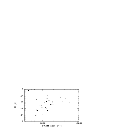
Figure 5: Parameters determined from variability analyses. Doubling time versus FWHM of $H\beta$ for NLS1 (filled circles) and normal Seyfert 1s (open circles).

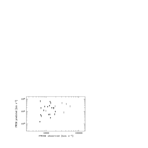
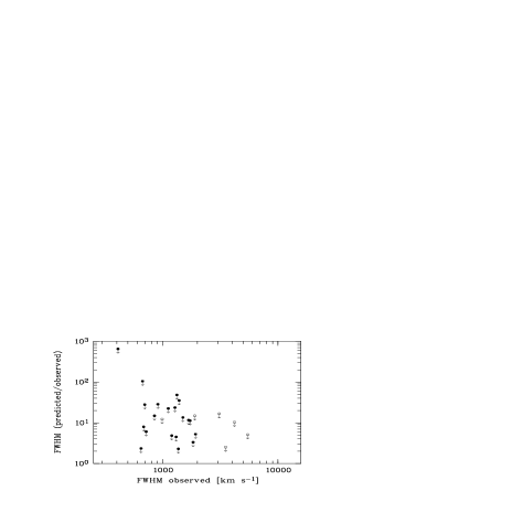
Figure 6: FWHM predicted from the model using X-ray variability analyses to set an upper limit on the black hole mass (Eq. (9)). Left Panel (6a): Prediced vs. observed FWHM. Right pannel (6b): FWHM(observed)/FWHM(predicted) vs. FWHM(observed) for the objects with doubling times (Eq. 14)

An upper limit for the black hole mass is given by (e.g. Wandel & Mushotzky 1986)

$$M(\Delta t)<(c^{3}/10G)\Delta t\simeq 10^{4}\Delta t\ M_{\hbox{$\odot$}},$$

where $\Delta t$ is in seconds. This relation assumes that the bulk of the X-ray continuum is emitted within 5 Schwarzschild radii, and that the variability is not affected by beaming or relativistic motions (cf. Boller et al. 1997 for an example of relativistic boosting effects in a radio-quiet, ultrasoft NLS1).

Using the doubling time as the characteristic time for variability we determine upper limits for the black hole mass for those objects of BBF96 and Wandel & Mushotzky (1986) whose continuum luminosities have been observed to vary significantly. Fig. 5 gives the doubling time (we have extrapolated amplitude variations linearely to a factor of 2 to determine $\Delta t$) versus the observed FWHM. Although there is some scatter, there is a strong indication for an increase of the doubling time with observed FWHM. This may indicate that NLS1 tend to have lower-mass black holes than ordinary Seyfert 1 galaxies.

Finally, for the objects with an established doubling time and mass upper limit, we may calculate the model velocity without having to assume any $L/M$ relation. Combining Eqs. (7) and (12) we have

$$FWHM<(3500km/s)\left(\frac{\Delta t}{10^{4}s}\right)^{1/2}\left(\frac{\alpha}{\alpha-1}\right)^{1/4}L_{x45}^{-1/4}.$$

Fig. 6a shows the predicted FWHM upper limits, and 6b - the ratio FWHM(observed)/FWHM(predicted), vs. FWHM(observed) for the objects with doubling times. We see that the predicted FWHM is larger than the observed one by an average factor of 10, which is not surprising, considering that the variability method gives only an upper limit for the mass. Similarly to the photoionization method, also here the ratio shows a slight anticorrelation with the observed FWHM.

5 Summary and Discussion

5.1 Basic Model

We derive a simple theoretical model which explains the observed distribution of line width and spectral index for Seyfert 1 galaxies. The observed velocity dispersion is determined by the mass of the black hole and the broad line region radius. Sources with steep X-ray spectra (for a given luminosity) have a stronger ionizing power than flat-spectrum sources, which implies that the BLR is formed at relatively larger distances from the central source, and hence has a smaller velocity dispersion and a smaller observed FWHM.

5.2 Model Parameters

The model predicts a particular distribution of the luminosities in the three dimensional FWHM-$L_{x}-\alpha$ space, which is essentially confirmed by the data. The FWHM also depends on the parameters $U,n,E_{0}$ (and perhaps other parameters we are not aware of), as shown in Eqs. (8) and (9). All those parameters, however, cannot be observed directly or are not available for the individual objects, so we develop and test the explicit teoretical relation for the observables that are available for the individual objects in our sample, and show that the data is consistent with the theoretical relation we derive. The dependence on the other parameters is kept in the equations, but because of our observational ignorance we assume that all objects have the same values for those parameters. This choise leads to an implicit error, which contributes to the scatter in Fig. 3. Because of the weak dependence on the parameters, the expected error is relatively small, of the order of 3 for the expected parameter range.

In addition to the scatter in the parameters, there may be also a systematic dependence on some of the observables, which would lead to a dependence of the predicted/observed FWHM ratio. This is shown to be the case for the parameter $\eta_{x}=L_{x}/L_{Edd}$, and is treated in Sect. 3.2. In principle, also the other parameters may systematically depend on some variable, but the data required to check this (e.g. separate determinations of $Un_{e}$) for individual objects are not yet available.

5.3 Observational Bias

BBF96 searched the literature for reports of NLS1 and found 46 in total. 32 of these NLS1 were located in in the fields of view of ROSAT pointings in the public archive. Only one of these 32 objects was not found above a 5 $\sigma$ detection limit. Walter & Fink 1993 selected all Seyfert 1 type AGN with more than 300 counts in the ROSAT All-Sky Survey data which were observed at least once in the ultraviolet with IUE. Although the selection of broad and narrow-lined AGN is based on these special selection criteria, there are no obviousg selection effects that can account for the absence of broad line AGN with steep soft X-ray spectra. The measurements in the photon index and the H_β values are totally independent so that there is no obvious way a spurious correlation could be induced.

5.4 Independent determination of the Mass

Estimating an upper limit for the central mass directly from X-ray variability data we find that AGN with narrow optical emission lines may have lower black hole masses than broad line AGNs (Fig. 5). In a separate work we will consider physical parameters leading to soft X-ray spectra to further improve our model. In order to test this mass estimate, it is possible to compare the BLR radius calculated from the ionizing luminosity (e.g. Eq. 2) or from reverberation mapping to the radius inferred from the observed FWHM and the mass estimated from the variability. Doing this indicates that the variability mass tends to be larger than the real mass for low narrow-line AGN (Wandel and Boller 1997).

5.5 What causes steep X-ray spectra in NLS1s?

We have shown that sources with a steep soft X-ray spectrum will have narrower broad lines than objects with flat spectra. A question we have not touched in this work is the cause for the observed steep X-ray spectra in many NLS1s. In principle, smaller central masses could produce steep soft X-ray spectra as follows. For a given accretion rate, lower mass black holes could yield a hotter accretion disk,which would radiate more energy in the soft X-ray band. X-ray reprocessing by the accretion disk would produce a soft X-ray spectrum (Matsuoka et al. 1990, Pounds et al. 1990) that extends to higher energies. This would make them appear to have steeper ROSAT spectra since there would be more flux in the soft X-ray band. This scenario will be considered in a separate work.

References

- [] Alexander, T., Netzer, H., 1994, MNRAS, 270, 781
- [] Boller, Th., Brandt, W.N., Fink, H. 1996, A&A, 305, 53 (BBF96)
- [] Boller, Th., Brandt, W.N., Fabian, A.C., Fink, H., MNRAS submitted; astro-ph/9703126.
- [] Clavel J. et al. 1991, ApJ, 366, 64.
- [] Kriss, G.A. 1988, Apj , 324, 809.
- [] Matsuoka et al. 1990, ApJ, 361, 440.
- [] Mushotzky, R.F. and Wandel, A. 1989, Apj , 339, 674.
- [] Netzer, H. 1990 in ”Active Galactic Nuclei”, Saas-Fee Advanced Course 20, eds. T.J.-L. Courvoisier and M. Major, Springer Verlag, Berlin, p. 57.
- [] Peterson, B.M. in ”Reverberation Mapping of AGN” eds. P.M. Gondhalekar, K.Horne, B.M.Peterson, SFASP 1995.
- [] Rees, M., Netzer H., Ferland, G.J. 1989. ApJ , 347, 640.
- [] Pounds, K. et al., 1990, Nature, 344, 132.
- [] Walter, R. and Fink, H.H. 1993, A&A , 274, 105.
- [] Wandel, A. 1996, in ”X-ray Imaging and Spectroscopy of Cosmic Hot Plasmas”, p. 307, ed. F.Makino, K. Mitsuda, Universal Academy Press, Tokyo .
- [] Wandel, A. 1997, ApJ Letters, 490, in press.
- [] Wandel, A. and Mushotzky, R.F. 1986, ApJ , 306, L61.
- [] Wandel, A. and Yahil, A. 1985, ApJ , 295, L1.
- [] Wandel, A. and Boller, Th. 1997, in ”Astronomical Time Series”, eds. D. Maoz et.al., Dordrecht: Kluwer, p. 255; astro-ph/9703198.