Linking Cluster Formation to Large Scale Structure

Abstract

We use two high resolution CDM simulations to show that (i) when clusters of galaxies form the infall pattern of matter is not random but shows clear features which are correlated in time; (ii) in addition, the infall patterns are correlated with the cluster’s surrounding Large Scale Structure; (iii) Large Scale Structure shows a mix of both filaments and sheets; (iv) the amount of mass in filaments is slightly larger for a low $\Omega$ model.

1 Introduction

Clusters of galaxies are well–studied despite their rarity because they are easy to find and are the largest known objects in approximate dynamical equilibrium. Furthermore, their current dynamics and their evolution appear to be dominated by the gravity of the unseen dark component.

The assumption that the formation of a galaxy cluster is dominated by gravity allows one to study clusters with collisionless N–body simulations. The dynamics is then well understood, and it is possible to simulate different cosmologies to investigate how cluster formation is affected by cosmological parameters. Only recently has it become possible to run simulations with high enough resolution to study details of cluster formation with high accuracy. Currently, two techniques are used. The first runs a cosmological N–body simulation with poor resolution, extracts a cluster from it and re–simulates the cluster with a multi–mass technique which gives high resolution on the cluster itself (for recent results see the comprehensive paper by Huss et al. 1997). Simulations like these can be done on high–end workstations. Their main disadvantage is that each simulation yields only one cluster. The second approach is somewhat simpler and runs a cosmological N–body simulation with high resolution throughout a large volume. This is only really practical on the latest generation of parallel supercomputers. In this case, however, one gets a large number of clusters in each simulation.

Simulations of the second type are particularly useful if one wants to investigate how the formation of a cluster is influenced by Large Scale Structure (LSS). This is the topic of this paper. We will study links between the formation of clusters within large high resolution N–body simulations and their surrounding LSS. In addition, we will address several aspects of the LSS itself, e.g., we will show that in these Cold Dark Matter (CDM) universes, both filaments and sheets can be found, and that it is possible to display these directly despite the large difference in their density. This is interesting because of the ongoing debate about how best to describe LSS. Sheets or walls (Geller & Huchra 1989, de Lapparent et al. 1986), filaments (Giovanelli et al. 1986), and mixes of these to produce a cell–like geometry (Jôeveer & Einasto 1987) have all been suggested. Bond et al. (1995) have shown that this mix already shows up in the overdensity pattern of the initial density field.

The outline of this paper is as follows. In section 2 we will introduce the simulations we use. The formation of clusters will be investigated in section 3. After selecting the clusters (sec. 3.1), their formation history will be constructed (sec. 3.2). This will then be studied in detail (sec. 3.3) using Aitoff projection maps and correlation functions. We link the formation process to LSS in section 3.4. Finally, mass fractions of the matter in the filaments are computed (sec. 3.5). Section 4 summarizes our results.

2 The Simulations

Our simulations were carried out using HYDRA, a parallel adaptive particle–particle particle–mesh (AP³M) code, developed within the VIRGO supercomputing consortium (For details on the code c.f. Couchman et al. 1995 and Pearce & Couchman 1997). The simulations were started on the CRAY T3D at the Computer Center of the Max Planck Society in Garching using 128 processors. Once the clustering strength required an even larger amount of total memory, they were finished on the T3D at the Edinburgh Parallel Computing Centre using 256 processors.

A set of four 256³ particle simulations with different cosmological parameters was run. These were designed primarily for another purpose and will be described in more detail in Kauffmann et al. 1997. From these two are taken, namely an $\Omega=1$ model, $\tau$CDM, with $h=0.5$, $\Gamma=0.21$ and a box size of 85 $h^{-1}$ Mpc, and an open $\Omega=0.3$ one, OCDM with $h=0.7$, $\Gamma=0.21$ and a box size of 141 $h^{-1}$ Mpc (As usual, the Hubble constant is expressed as $H_{0}=100h$ km sec^-1 Mpc^-1, and $\Gamma$ is the shape parameter of the CDM spectrum (c.f. Bond et al. 1984)). The models are normalized such that they yield the observed abundance of rich clusters by mass, i.e., $\sigma_{8}=0.6$ and $\sigma_{8}=0.85$ for $\tau$CDM and OCDM, respectively. All the models were run with the same phases so that objects are directly comparable.

These simulations are particularly useful for the purposes of this paper because they resolve clusters and their surrounding LSS very well. From the 50 output times which were stored we use the ones later than $z=1$. They are $z=$0.93, 0.82, 0.72, 0.62, 0.52, 0.43, 0.35, 0.27, 0.20, 0.13, 0.06, and 0.0.

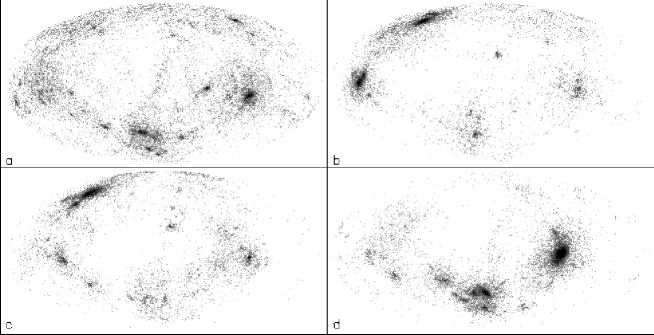
Figure 1: The infall pattern of matter onto a cluster in the $\tau$CDM model viewed from an hypothetical observer in the barycenter of the system. Shown are different time intervals: (a) $z=0.$ to $z=0.13$, (b) $z=0.13$ to $z=0.27$, (c) $z=0.27$ to $z=0.43$, and (d) $z=0.43$ to $z=0.62$.

3 The Formation of Clusters

3.1 The Selection of Clusters

The definition of a cluster adopted here is analogous to Abell’s criteria for the selection of clusters from galaxy catalogs. Of course, in a simulation clusters can be found using full 3D information. At $z=0$, high density regions are found using a standard friends–of–friends group finder with a linking length of 0.05 times the mean interparticle separation. Spheres with a radius of $r_{\rm A}\equiv 1.5\,h^{-1}$ Mpc (comoving) are put around the barycenters of those regions and all particles inside them are taken as members of the cluster. If two cluster centers are closer than $r_{A}$ the more massive one is taken and the other one deleted from the list. No recentering is done after such a step. From both models the ten most massive clusters are taken. The mass range of these clusters is from 2.7$\times 10^{14}h^{-1}M_{\odot}$ (3.5$\times 10^{14}h^{-1}M_{\odot}$) to 7.3$\times 10^{14}h^{-1}M_{\odot}$ (8.4$\times 10^{14}h^{-1}M_{\odot}$) for the $\tau$CDM (OCDM) model.

3.2 Construction of the Formation History

After having found the clusters the particles in each of them are marked in a list. Using this information they are extracted from the whole set of particles at all redshifts. After that two additional pieces of information are obtained for each particle: The time when it falls into the cluster and its position at that time. This is done in the following manner. With the above selection criteria a cluster is a spherical object with a radius $r_{\rm A}$ at any time. Let the current time be $z_{i}$. Going back to $z_{i-1}$, some of the particles which will be inside $r_{\rm A}$ at $z_{i}$ are still outside. Hence, these particles will fall into the cluster between $z_{i-1}$ and $z_{i}$. So for these particles $z_{i-1}$ as well as the position at this time are saved. As the center of the cluster we take the barycenter at $z_{i-1}$ of the biggest lump.

3.3 Investigating the Formation of the Clusters

Often the formation of a cluster is modeled by the spherical collapse of some high peak in the initial density field. However, previous studies, e.g. Tormen et al. [1997], have already shown that the actual formation process in hierarchical models is rather irregular. Instead of a steady accretion of matter, lumps fall onto a pre–existing object, a process well known in and typical of CDM models.

Here we study the build–up of clusters in more detail. A hypothetical observer is placed at the barycenter of each cluster. This observer watches the matter as it falls into the cluster. For spherical infall he would see matter coming in more or less randomly from all directions. For each observer, maps of the infall pattern are produced by plotting the positions of the particles at infall on an Aitoff projection. Figure 1 shows typical examples of such maps for a cluster in the $\tau$CDM simulation. From this some points can be made. (i) It is obvious that matter is not falling in uniformly over the sky as one would expect in a spherical infall model. Rather infall occurs from distinct directions. (ii) There is a tight correlation between the infall directions at different times. That is, the cluster forms by accretion from a few preferred directions.

In order to quantify this process we have computed the autocorrelation function of the infalling matter

$$1+\omega(\vartheta)=\frac{4\pi}{A(\vartheta)}\frac{N_{\rm PP}(\vartheta)}{N(N-1)}\,,$$ (1)

where $N_{\rm PP}(\vartheta)$ denotes the number of particle pairs separated by an angle $\vartheta+\delta\vartheta$, $A(\vartheta)=2\pi\sin\vartheta{\rm d}\vartheta$ is the size of the annulus, and $N$ is the total number of particles in the sample. Obviously, $\omega(\vartheta)$ is the excess probability of finding a particle pair with separation $\vartheta+\delta\vartheta$ in the simulations compared with spherical infall.

Figure 2: The auto correlation functions of the matter shown in fig. 1 for the same time intervals used in the four panels of fig. 1. Also shown is the prediction for spherical infall.

Figure 2 shows the autocorrelation functions for the infalling matter of the cluster in fig. 1 and for random spherical infall. For small angles all the curves have a peak. This just reflects the particle clumps seen in fig. 1. The strength of the peak directly reflects the amount of matter in these clumps. For some of the curves, peaks also appear at larger angles. For example, curve (b) has a second peak around 60^∘. This reflects the angle between the two most massive objects in fig. 1(b).

These curves can be compared directly to the correlations of matter between different maps, as quantified by the cross–correlation function

$$1+\tilde{\omega}(\vartheta)=\frac{4\pi}{A(\vartheta)}\frac{N_{\rm P_{1}P_{2}}(\vartheta)}{N_{1}\cdot N_{2}},$$ (2)

where $N_{\rm P_{1}P_{2}}$ denotes the number of pairs of a particle from map 1 and one from map 2 separated by an angle $\vartheta+\delta\vartheta$, where $A(\vartheta)=2\pi\sin\vartheta{\rm d}\vartheta$ is the size of the annulus again, and $N_{1}$ and $N_{2}$ are the number of particles in the maps 1 and 2, respectively.

Figure 3: The cross correlation between pairs of maps from fig. 1. Also shown is the result expected for uncorrelated maps (dotted).

Figure 3 shows cross–correlations between pairs of maps from fig. 1. These have similar scale but are generally weaker than the autocorrelations. This can be seen by comparing the maps directly, too. The behaviour for this particular cluster is typical for both the auto– and cross–correlations in the infall patterns of all clusters in both the $\tau$CDM and OCDM model. Not a single case was found which deviates qualitatively from it.

From the above, it is apparent that correlations between the infall patterns at different times are strong. The question now is whether one should expect to find such a correlation? From previous studies, e.g. Tormen et al. 1997, it is clear that clusters form by the accretion of haloes. This is already reflected by the discussion above. The question left is: Why is the infall pattern of matter between so many and so different redshift intervals correlated? This may be rephrased as: Is there a connection between the infall pattern and LSS itself? This will be discussed in the next sections.

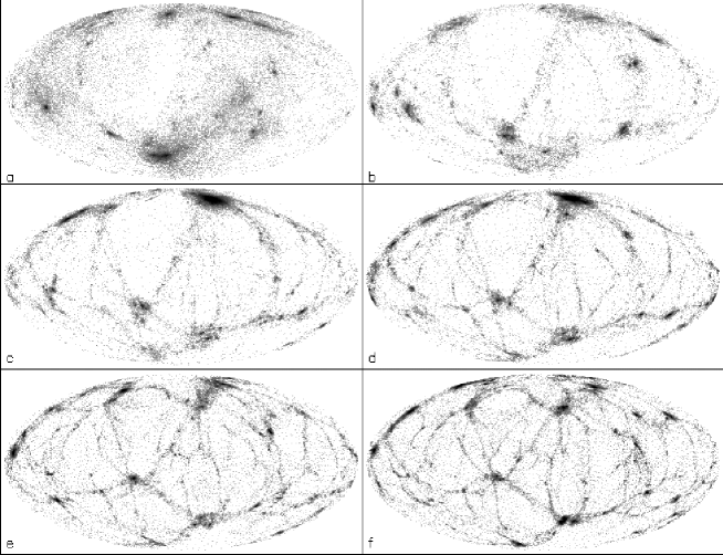
Figure 4: The LSS around the cluster shown in fig. 1 viewed from an hypothetical observer at the barycenter of the cluster at $z=0$. Shown are shells at 1.5 to 3.0 (a), 3.0 to 4.5 (b), 4.5 to 6.0 (c), 6.0 to 7.5 (d), 7.5 to 9.0 (e), and 9.0 to 10.5 $h^{-1}$ Mpc (f) from the cluster center.

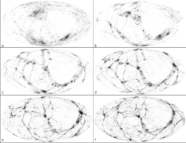
Figure 5: The LSS around another cluster from the $\tau$CDM simulation shown using the same representation as in fig. 4.

3.4 Connecting Cluster Formation and Large Scale Structure

From the above it is obvious that the during formation of a cluster matter falls in from well–defined directions. What is the connection between these dierections and Large Scale Structure? In order to investigate this the distribution of matter surrounding the clusters at $z=0$ is obtained as follows. Around the clusters we put onion–like shells of thickness $1.5\,h^{-1}$ Mpc are put. All particles in a shell are extracted. The hypothetical observer at the cluster center draws maps of these particles, i.e., LSS is viewed from the center of each cluster.

Figure 6: The combined cross correlation between the infall patterns of the clusters in the $\tau$CDM and OCDM simulations and their surrounding LSS.

Figure 4 shows maps for shells surrounding the $\tau$CDM cluster which we analyzed in figures 1 to 3. Again, these maps are typical of those found for all the clusters. From the maps some points can be made. (i) There exist density enhancements in the distribution of the particles which only marginally change their locations from map to map. Most of them are more or less circular. These must clearly be filaments extending outwards from the cluster. In addition, fig. 4 shows another interesting feature. There are enhancements which connect the filaments and also extend outwards from map to map, but are less dense. Figure 5 shows the LSS around a different $\tau$CDM cluster where these connections between the filaments are very strong. There is a U–shaped broad band in the right part of five of the six maps. This object is obviously a sheet. One has to note that filaments can be found in all of the cluster maps. There are connections between them in all maps, too. However, impressive examples of sheets like the one in figure 5 are rare. (ii) When comparing the maps in figure 4 with the one in fig. 1 one can see that the big clumps fall in along the filaments. This is not only true for the lowest redshift range but for the earlier ones, too. Even at a redshift of 0.6 infall onto clusters is tightly coupled to LSS at $z=0$.

In order to quantify this connection a little bit further, the angular cross correlation functions between the combined infall maps of the cluster and the LSS maps are computed for each cluster in each cosmology.

Figure 6 shows cross correlations between the infall patterns and surrounding LSS for the ten $\tau$CDM and OCDM clusters. These are averaged over the redshift ranges and radii shown in fig.s 1, 4, and 5. Very similar cross correlations are found for other time and radius intervals. This mean cross correlation behaves in a similar manner for the cross correlations between the different maps in fig. 3. There is indeed a well defined correlation between the infall onto clusters and their surrounding LSS. This correlation does not depend on $\Omega$.

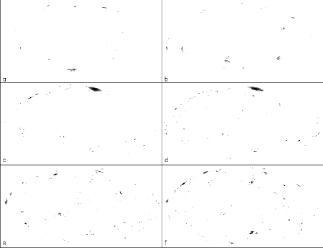
Figure 7: A different representation of fig. 4 where only the lumps (filaments) show up.

3.5 Fraction of Mass in the Peaks

What is the amount of mass which can be seen in the various structures in the above maps? In order to answer this question we have computed the amount of mass inside the dark spots. This is done by using a standard friends–of–friends group finder on the sets of points on the unit sphere from which the above maps were drawn. As linking parameter a value of $b=0.2$ times the mean interparticle separation is taken. All objects with 20 or more particles are considered as big groups.

Table 1: Fractions of mass in the dark spots for the maps in fig. 4 and 5. Given are the total mass fractions ($f_{\rm all}$) as well as the mass fractions of the two biggest spots ($f_{1}$ and $f_{2}$) for the different radii.

Radius	Fig. 4			Fig. 5
$[$Mpc/h$]$	$f_{\rm all}$	$f_{1}$	$f_{2}$	$f_{\rm all}$	$f_{1}$	$f_{2}$
1.5 – 3.0	11%	5%	2%	13%	9%	2%
3.0 – 4.5	22%	3%	3%	24%	4%	4%
4.5 – 6.0	52%	42%	2%	28%	10%	3%
6.0 – 7.5	45%	32%	1%	34%	5%	4%
7.5 – 9.0	32%	7%	4%	43%	17%	3%
9.0 – 10.5	39%	8%	5%	32%	6%	2%

Table 1 gives the fraction of mass inside such big dark spots for the figures 4 and 5 ($f_{\rm all}$). Also shown is the fraction of mass in the two most massive spots in each map ($f_{1}$ and $f_{2}$). Typically, about a third of the mass lies in filaments at the overdensity of $\sim$20 picked out by our choice of linking length.

Fig. 7 shows a representation of the maps in fig. 4 where only the particles in these dark spots, i.e., the filaments are plotted. From this it is apparent that filaments are clumpy structures rather than homogeneous cylinders.

Performing a similar analysis for the infall patterns onto clusters gives results which vary more strongly between clusters and time intervals. E.g., for the cluster shown in fig. 1 the fractions of mass in the dark spots are 5%, 15%, 30%, and 51% for the maps (a) to (d), respectively. This scatter between 5% and around 55% was quite typical for clusters in both the $\tau$CDM and the OCDM sample.

For the whole $\tau$CDM (OCDM) cluster sample the averaged mass fractions in the filaments are 14% (14%) , 29% (35%), and 42% (46%) for shells beginning at radii 1.5, 3.0, and 4.5 $h^{-1}$ Mpc. These stay constant at around 40% (48%) for larger radii. There is a slightly larger mass fraction in the filaments in the low $\Omega$ model.

4 Conclusions

Our study of the formation process of clusters and its connection with LSS has yielded several conclusions. (i) In CDM universes, clusters form by the accretion of collapsed haloes onto other pre–existing haloes. This occurs from preferred directions. These directions do not change much with time. (ii) There is a correlation between the formation process of a cluster and its surrounding LSS. Qualitatively speaking, matter falls in mainly from filaments and sheets. The filaments show up as clear density enhancements in our 2D projections. They extend outwards from the cluster center and are connected by less dense sheets of matter. Because of their considerably lower density contrast these sheets are nearly impossible to find in 3D representations of N–body simulations. Our representation clearly shows that both filaments and sheets do exist in simulations. Quantitatively speaking, the amount of mass in the filaments is around 40% and 48% of the total mass for radii from 4.5 to 10.5 $h^{-1}$ Mpc in the $\tau$CDM and OCDM model, respectively. At smaller radii, it is around 30%. However, the mass distribution is dominated by lumps inside the filaments. (iii) The only difference we could find between the $\tau$CDM and the OCDM model is in the amount of mass in the filaments, it is slightly larger for the OCDM model.

The formation process of each cluster is governed by its surrounding LSS. The internal properties of the cluster may change during its formation, as shown by Tormen et al. [1997], but this is no completely chaotic process but is linked to the LSS. LSS itself appears to be a mix of both filaments and sheets in CDM universes at least in the representation we have emphasized in this paper. These simulation results clearly reinforce the Cosmic Web picture of structure formation proposed by Bond et al. (1995)

References

- [1984] Bond J.R., Efstathiou G., ApJ, 285, L45 (1984)
- [1995] Bond J.R., Kofman L., Pogosyan D., astro-ph/9512141
- [1995] Couchman H.M.P., Thomas P.A., Pearce F.R., ApJ, 452, 797 (1995)
- [1986] de Lapparant V., Geller M.J., Huchra J.P., ApJ, 302, L1 (1986)
- [1989] Geller M.J., Huchra J.P., Science, 246, 897 (1989)
- [1986] Giovanelli R., Haynes M., Myers S.T., Roth J., AJ, 92, 250 (1986)
- [1997] Huss A., Jain B., Steinmetz M., submitted to MNRAS
- [1978] Jôeveer M., Einasto J., in IAU Symp. 79, The Large–Scale Structure of the Universe, eds. Longair M.S., Einasto J. (Dordrecht: Reidel), 241 (1978)
- [1997] Kauffmann G.A.M., Colberg J.M., Diaferio A., White S.D.M., in preparation
- [1997] Pearce F.R., Couchman H.M.P., Hydra: A parallel adaptive grid code, submitted to New Astronomy (1997)
- [1997] Tormen G., Bouchet F.R., White S.D.M., MNRAS, 286, 865 (1997)