Search and analysis of small scale structures in two X–ray clusters of galaxies

Abstract

We present a refinement of the wavelet analysis technique for the detection and characterisation of small scale features embedded in a strongly varying background. This technique handles with particular care the side effects of non-orthogonality in the wavelet space which can cause spurious detections and lead to a biased estimate of source parameters. This novel technique is applied to two ROSAT PSPC pointed observations of nearby clusters of galaxies, A1367 and A194. We find evidence that the case of A1367 is not unique and that galaxy-scale X–ray emission could be a quite common property of clusters of galaxies. We detect 28 sources in the field of A1367 and 26 in the field of A194. Since these numbers are significantly larger than those expected from the $\log N-\log S$ relation in the field, most of the sources are expected to be associated with the cluster itself and indeed several identifications with galaxies are possible. In addition, CCD observations have revealed that two X–ray sources in the field of A194, classified as extended by the multi-scale analysis, are very likely associated with two background galaxy clusters at intermediate redshift.

1 Introduction

The study of the X–ray emission from clusters of galaxies plays a central role in understanding the origin of the intra-cluster medium (ICM), its interaction with the cluster galaxies and the physics related to the merging processes in the ICM. A first detection of X–ray emission from the single galaxies in a cluster, beyond Virgo, was made in A1367 by Bechtold et al. (1983, hereafter BAL) using the High Resolution Imager (HRI) and Imaging Proportional Counter (IPC) instruments on board Einstein. Following this work, optical observations have shown that in such X–ray emitting galaxies high temperature coronal gas coexists with cold HI gas, although the latter is found to be significantly underabundant when compared to X–ray quiet cluster galaxies (Chincarini et al. 1983).

The detection of individual galaxies in clusters has been limited so far by the angular resolution of the X–ray instruments. Although the next generation of X–ray telescopes (e.g. AXAF, JET–X, XMM) will facilitate these studies, the use of a flexible detection algorithm is the main ingredient to generate reliable catalogs of X–ray emitting galaxies in clusters, by separating the small scale features from the strong diffuse cluster emission, and provide accurate measurements of characteristic sizes and fluxes.

A previous attempt to apply a wavelet transform-based algorithm to a new pointed ROSAT observation of A1367 was carried out by Grebenev et al. (1995, hereafter GAL). They generated a catalog of point sources and discuss possible identifications of optical counterparts in the cluster field. In this work we extend the GAL analysis and present an improvement of the wavelet detection technique which is designed to minimise the side effects of the transform and to deal with the a strongly-varying background and source confusion. The method is then applied to the search for small-scale X–ray emission in two clusters of galaxies, A1367 and A194.

Our work is organised as follows: in section 2 we briefly outline the wavelet algorithm while in section 3 we detail our analysis. Results of individual clusters are given in section 4; section 5 contains a brief summary.

2 The Method

The method we present is based on the wavelet transform, a mathematical tool which has been recently used for multi-scale data analysis in different astronomical applications. For the complete theory of wavelet operators, we refer to some of the extensive reviews published in the literature, e.g. GAL and Slezak et al. (1995). The wavelet transform (hereafter WT) of a real function $f$ is defined as the convolution product (more precisely as the scalar product) between the function and a class of analysing wavelets $\{\psi_{a,b}\}$, all derived by translation and dilation from a single function, generally complex (but in our case real), called mother wavelet, which has to fulfill the condition (in the discrete approximation):

Figure 1: Example of non-orthogonality in scale: the six panels show an elliptical King profile [panel (a)] and its WT at five increasing scales [panels (b)-(f)]. It can be seen that the coefficients of the small scale transforms [panel (b)-(d)] are not equal to zero, as discussed in the text. The vertical axes of panels (b)-(f) have the same dimensions.

$$\sum_{i,j}\psi_{i,j}=0$$ (1)

for a two-dimensional transform.

The discrete approximation of the WT can hence be written as a convolution in $l^{2}$:

$$w_{i,j,a_{n}}={1\over{a_{n}^{2}}}\sum_{k,l}f_{k,l}\;\psi_{{{i-k}\over{a_{n}}},{{j-l}\over{a_{n}}}}$$ (2)

where, for a proper sampling, the scales $a_{n}$ must be chosen according to:

$$a_{n}=(2^{m})^{n}\qquad\qquad\qquad m\in{\bf Z}$$ (3)

with $m$ fixed.

As pointed out by many authors, the most appealing property of the WT resides in its capability of decomposing $f$ in a certain number of functions, each representing the features of $f$ at a given scale, leaving unaffected the positional information.

The WT has another great advantage, it gives an exact estimate of the significance of correlated multi-pixel enhancements, regardless of the amplitude of the enhancement, even in the presence of non-flat background components. Moreover, this process does not require an estimate of the local background since the variance in the transform pixel by pixel can be calculated without assuming a background model.

The formula for the background variance is given in GAL:

$$\sigma^{2}_{i,j,a_{n}}={1\over{a_{n}^{4}}}\sum_{k,l}{\sigma_{f}^{2}}_{k,l}\;\psi^{2}_{{{i-k}\over{a_{n}}},{{j-l}\over{a_{n}}}}$$ (4)

where we have used the symbol $\sigma$, typical of the Gaussian distribution, because it can be shown that the single WT coefficients are distributed according to a Gaussian statistics with standard deviation given by Equation 4 (Lazzati 1996). This result is exact if $f_{i,j}$ have a Gaussian distribution and is a very good approximation for a Poisson distribution if the mean number of counts is sufficiently large ($\lower 2.15277pt\hbox{$\;\buildrel>\over{\sim}\;$}20$) or the scale $a_{n}$ is sufficiently large.

Despite all these properties, the WT has a major disadvantage which usually tends to be neglected (e.g. GAL) or overemphasised (e.g. Pando & Fang 1996): the wavelet bases commonly adopted for astronomical purposes are not orthogonal, neither for rescaling nor under translations.

Figure 2: Sources detected in the field of A1367: crosses and diamonds represent detections before and after the King profile subtraction, respectively. The center of the cluster is at (0,0). See the text for the relevance of crosses without diamonds and diamonds without crosses.

2.1 Non-orthogonality in space

In the analysis of astronomical images, the non-orthogonality under translations has the effect of producing a correlation between the uncertainties on WT-space coefficients. In the mere identification of sources this is not a major problem, since the statistical significance of detections comes from the value of a single coefficient. However, it is mandatory to take into account this effect if standard fitting procedures have to be used.

Problems arise for near sources since the tail of the first source can affect the significance of the second. This is not an easy problem, but it has been shown (Rosati 1995; Rosati et al. 1995) that WT based detection algorithms deal the confusion problem better than other techniques commonly used in X–ray astronomy, such as the sliding box technique.

Given the fact that the number of independent points in a single-scale transform is not known, it is not possible to derive analytically the expected number of spurious sources in the detected sample, despite the Gaussian character of the statistic. Simulations must be performed to assess the significance of the detection as in GAL. These simulations however are rather difficult, due to the lack of a consistent model for the background component (we call background also the large-scale emission from the ICM). In this work we prefer to give the significance of each single source, i.e. we quote for each source the probability (in units of $\sigma$) of spurious detection.

2.2 Non-orthogonality in scale

A more serious problem is the non-orthogonality among different scales which causes large scale features to affect the coefficients of the small scale transforms. This effect is particularly important when we try to detect small and faint scale features embedded in a strong, large scale component.

As an example, we can consider the WT of a King profile modeling the cluster diffuse X–ray emission. It can be noticed that the transform has a maximum at its natural scale, but all the other scales have non-zero coefficients (see Figure 1). Since the operator is linear (see Equation 2), the transform of the superposition of a small scale feature (e.g. a galaxy) on the King profile in Figure 1 will be the sum of the transforms of the King profile and that of the small feature. The way how the significance of a small-scale feature is altered by the presence of the King profile depends on the position, since the transform of the profile is positive in the center and negative in an annulus around it. As a result, we overestimate the significance of small scale structures near the center of the cluster and underestimate that of sources in the outskirts.

3 The Analysis

We consider here the ROSAT Position Sensitive Proportional Counter (PSPC) observations of two clusters of galaxies (A194 and A1367), characterised by relatively small distances and long exposure times. In Table 1 we report the properties of these clusters and of their ROSAT observations.

Table 1: Properties of clusters and of ROSAT observations.

Name $R^{a}$ Redshift $BM\,^{b}$ Obs. ID Exp. (s) A194 0 0.0178 II rp800316 16317 A1367 2 0.0215 II-III rp800153 18224

^a Richness class

^b Bautz–Morgan type

3.1 Data reduction

The reduction of the ROSAT PSPC data has been performed with the method described by Snowden et al. (1992; 1993; 1994) and Plucinsky et al. (1993). The complete treatment takes into account the long and short term enhancements of background, the solar afterpulse and particle contamination, and the energy-dependent correction for vignetting and exposure time.

In order to oversample the PSPC Point Spread Function (PSF), the standard ESAS software (Snowden 1995) has been generalised to produce images with smaller pixel size (Lazzati 1996). In the following we analyse images in the hard band ($0.4-2.0$ keV) with a pixel size of 8 arcsec.

Figure 3: FWHM of detected sources compared to the PSPC PSF FWHM depending on the off-axis angle. The model for the PSF (solid line) is accurate up to $\theta\leq 18^{\prime}$. Dashed lines represent $3\,\sigma$ confidence level for the PSF model. A1367 field is the upper panel, A194 the lower.

Our source detection technique utilises the discrete WT based on the multi-resolution theory (Farge 1992) and the “à trous” algorithm (Bijaoui & Giudicelli 1992). The latter uses the ‘mother’ developed by Slezak et al. (1995), which can be analytically approximated with the difference of Gaussians:

$$\psi_{j,a,b} = 2\pi\Big{[}A\,\sigma_{A}^{2}\,G(x,y,a,b,2^{j}\sigma_{A})-$$ (5)

$$- B\,\sigma_{B}^{2}\,G(x,y,a,b,2^{j}\sigma_{B})\Big{]}$$

where

$$G(x,y,x^{\prime},y^{\prime},\sigma)=\frac{1}{2\pi\,\sigma^{2}}\,e^{\frac{(x-x^{\prime})^{2}+(y-y^{\prime})^{2}}{2\sigma^{2}}}$$ (6)

$A$ and $B$ are the normalisation factors and $\sigma_{a}$ e $\sigma_{b}$ the widths of the two Gaussians.

Figure 4: Color–color diagrams for the most luminous sources in the field of A1367 (upper panel) and A194 (lower panel). The softness ratio is defined as the ratio between the flux in the bands $(0.11-0.28)$ keV and $(0.28-1.2)$ keV, while the hardness ratio as the ratio between bands $(1.2-2.04)$ keV and $(0.28-1.2)$ keV. We expect sources associated with cluster objects to be hard due to the low energy absorption of the galactic interstellar medium ($N_{H}\sim 5\times 10^{20}$ cm^-2). Sources associated with cluster galaxies are marked with an asterisk.

3.2 Large scale emission

In order to correct for effects of the WT non-orthogonality (see section 2.2) and remove the cross-talk between the largest dominant scale and the small scale features, we fit and subtract an elliptical two-dimensional King profile from the original data. The fitting procedure is performed after masking regions flagged as compact sources or substructures by a first run of the detection algorithm. The best fit model is then subtracted and the residual image used for further analysis.

A great amount of study has been devoted to test the reliability of the two-dimensional fitting. Two possible solutions were explored in order to overcome the poor statistics in the external regions of the cluster. A first simple approach is to fit the image assuming Poissonian errors. This has the disadvantage of introducing a bias in the fitting procedure since negative deviations are weighted more than positive ones, thus producing an annulus with an excess of counts in the residual image.

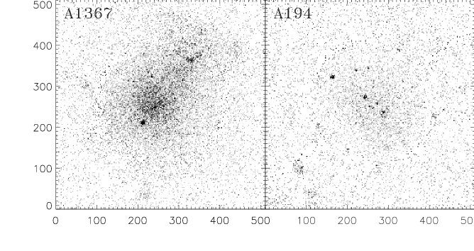
Figure 5: X–ray images of the two clusters analysed in the text. The fields are $68^{\prime}$ across, the pixel size is $8^{\prime\prime}$.

In order to obtain a better statistics without compromising the resolution, we have preferred to fit the King model to the original image smoothed with a bidimensional Gaussian (see also BAL). The reliability of this non standard procedure has been confirmed through a large set of simulations from which we have verified that the fitted and the true parameters are in good agreement as long as the size of the smoothing function is comparable to the detector PSF.

The outlined procedure, when compared to a cluster profile subtraction and detection in real space, has the following advantages:
a) the WT space is less affected by residuals from the large scale subtraction;
b) the WT algorithm is efficient also in cases where the standard deviation is not constant over the analysed field;
c) the WT algorithm proves to be very powerful for multi-scale source detection.

The importance of the cluster profile subtraction, i.e. the fact that we have to properly take into account the background signal to assess correctly the significance of detections, is illustrated in Figure 2. We show the sources detected at a $4\,\sigma$ level in one of the most studied clusters of galaxies, A1367 (BAL; GAL). Crosses and diamonds represent the sources detected before and after the subtraction of the fitted King profile, respectively. We note that the majority of the sources are detected in both cases, however in the central region (where the cluster emission is higher) differences can be found. The three central detections marked with a simple cross have a significance lower then $4\,\sigma$ but were enhanced above this threshold because of the coincidence with the peak of the cluster emission. The two sources marked with open diamonds are significant ($>4\,\sigma$) features suppressed by the negative wings of the cluster emission transform (see Figure 1). This example elucidates the importance of taking into account the diffuse cluster emission which can seriously affect the significance of source detections in the central regions.

Figure 6: Ratio between the surface density of detected sources with and without the King profile subtraction described in the text. Data are obtained from a set of 100 simulations of an A1367-like image with 150 compact sources superimposed.

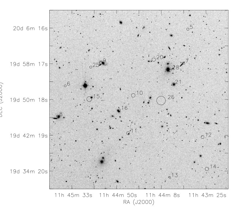
Figure 7: X–ray sources detected in the central $40^{\prime}\times 40^{\prime}$ of A1367 field overlaid on the relevant Digital Sky Survey (hereafter DSS) plate. The radii of circles represent the $3\,\sigma$ confidence radius on the central position of the X–ray source. The image has been corrected for boresight errors ($\sim 14^{\prime\prime}$; see text).

To test the influence of this effect, we have simulated a set of 100 images of an A1367-like cluster with the superposition of 150 compact sources distributed along a power-law $\log N-\log S$ with index $\alpha=-2.5$. We have performed the source detection with and without the King profile subtraction. In Figure 6 the ratio of the radial surface density profiles of detected sources in the two realisations is shown. in the central region of the image the number of sources detected without the King profile subtraction is up to three times greater than that of sources detected with our method. In the outskirt of the cluster, without a careful handling of the negative wings, up to $20\%$ of the sources are missed.

This problem has been faced in a recent paper by Damiani et al. (1997a, b) who calculate background maps at each scale by smoothing the image with different widths of the window. With this method, large features are seen as background at the lower scales, whereas small scale features are averaged in the upper scales. However the influence of the cross talks between different scales cannot be solved.

In a completely different approach, Bijaoui et al. (1995), Rue & Bijaoui (1996), Pislar et al. (1997) have discussed a restoration algorithm based on WT coefficients which does not need any parametrisation of the source shape. Similarly, Vikhlinin et al. (1997) subtract the small scale features from the WT before the computation of the larger scale coefficients.

3.3 Characterisation of detected sources

To characterise the detected sources, we developed a multi-scale fitting method (Lazzati et al. 1997; Campana et al. 1997). The basic formula of this method is the WT of a Gaussian source that, following equation 6 and given the mother of equation 5 can be written:

$$\tilde{f}(a,b) = 2\pi\,I_{0}\,\bigg{[}A\,\sigma_{A}^{2}\,G\Big{(}a,b,x^{\prime},y^{\prime},\sqrt{\sigma_{2}+2^{2j}\sigma_{A}^{2}}\Big{)}-$$ (7)

$$- B\,\sigma_{B}^{2}\,G\Big{(}a,b,x^{\prime},y^{\prime},\sqrt{\sigma^{2}+2^{2j}\sigma_{B}^{2}}\Big{)}\bigg{]}$$

where $I_{0}$ is the total number of source counts and $\sigma$ its width.

In this approach the WT of a Gaussian source is fit to the image transform at all scales simultaneously. This allows us to characterise in a single operation the multi-scale and two-dimensional behaviour of the detected sources, using all the available information. Thus we obtain the most accurate determination of the interesting parameters: position, size and count-rate. Unfortunately, due to the high spatial correlation of WT parameters, especially at the largest scales, a simultaneous fit of all coefficients would be time-expensive and redundant. Moreover, uncertainties of adjacent pixels are correlated and standard fitting techniques should not be used.

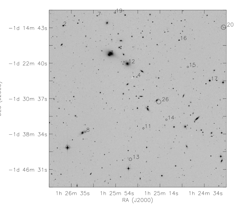
Figure 8: X–ray sources detected in the central $40^{\prime}\times 40^{\prime}$ of A194 field overlaid on the relevant DSS plate. The radii of circles represent the $3\,\sigma$ confidence radius on the central position of the X–ray source. The image has been corrected for boresight errors ($\sim 8^{\prime\prime}$; see text).

These problems are simultaneously solved with a decimation process which leads to a subset of coefficients with properties analogous to monodimensional orthogonal wavelets. Named $\tilde{a}$ the most significant scale for a detected source, we consider only coefficients taken at the scales $\{\tilde{a}/2,\tilde{a},2\tilde{a}\}$. We do not extend the analysis to additional scales since smaller scales ($<\tilde{a}/2$) are dominated by noise, while larger ones ($>2\tilde{a}$) are affected by source confusion. From the WT at these three scales we then extract a subset of coefficients with a spacing roughly equal to the correlation length of the WT at a particular scale and a spatial support matching the one of the mother at the most significant scale. In addition the denser sampling at lower scales allows any aliasing problem to be avoided.

This new technique presents different advantages with respect to the ones already used in X–ray analysis, i.e. maximum fitting (see GAL) or scale by scale $\chi^{2}$ minimisation (see Rosati 1995). First the 4-dimensional fit provides us with a fast, consistent and unique determination of all parameters without the loss of information involved in the maximum fitting technique or the a posteriori weighted sum of different scale coefficients needed in the scale by scale characterisation. Second, the measurement of the positions can be refined during the fitting procedure (unlike in the GAL technique) and the presence of nearby detections is easily treated with a simultaneous multi-source fitting. Finally, the errors in the estimated parameters are automatically obtained from the covariance matrix without referring to $\chi^{2}$ space. This fundamental result is due to the fact that the subset of the WT coefficients obtained after the decimation is almost orthogonal and Gaussian distributed.

A large set of simulations has been carried out in order to test the reliability of the source parameters and related errors (Lazzati et al. 1997). These simulations have revealed that as long as the WT coefficients are sufficiently Gaussian distributed, the procedure works very well. With background values below $\sim 5\times 10^{-2}$ counts pixel^-1 the distribution in the lowest scales of WT space becomes increasingly Poissonian and the covariance matrix gives underestimated errors, even if parameter determination remains reliable.

A rough distinction between point-like and extended sources can be made by comparing the source width (FWHM), as derived by the fitting procedure, and the PSPC PSF at a given off-axis angle (see Figure 3). The solid line is a model of the behaviour of the PSPC PSF FWHM taken from Rosati (1995). Sources with a FWHM larger that the local PSF FWHM at a $>3\,\sigma$ level are classified as extended in Tables 2 and 3. It is important to stress that, since this model is valid only inside the PSPC support ring (vertical dashed line in Figure 3), classification of sources at larger angles is questionable. In Tables 2 and 3 these classifications are marked with a $.

A spectral analysis has also been performed in order to better characterise the physical properties of the X–ray sources. Due to the low signal-to-noise of these objects only colour–colour diagrams have been constructed rather than X–ray spectra (see Figure 4). In this Figure, sources associated with cluster members (i.e. positionally coincident with galaxies, see below) are marked with an asterisk. Even though the colour information is not sufficient to fully discriminate between different spectral properties, we note that the softness–ratio of marked sources is lower than the mean value of the sample and is consistent with the value from a source with a bremsstrahlung spectrum with $T\lower 2.15277pt\hbox{$\;\buildrel<\over{\sim}\;$}2$ keV, absorbed with the galactic column density in the direction of the target.

4 Individual clusters

4.1 A1367

Table 2: Parameters of the small-scale features detected in A1367 field.

Name	Sign.	R.A.	DEC.	Error boxa	FWHM	Count rateb	Class.c	Other work	Optical
	$(\sigma)$	(J2000)	(J2000)	(arcsec)	(arcsec)	(c ks-1)		sourcesd	identificationse
1	32.6	11h 45m 05.0s	19∘36′ 22′′	0.8	$38\pm 2$	$256\pm 8$	P	P8 G24	54
2	8.3	11h 45m 01.0s	19∘12′ 49′′	3.2	$160\pm 5$	$47\pm 2$	P$
3	7.1	11h 46m 24.0s	19∘48′ 28′′	4.0	$114\pm 7$	$18\pm 2$	P$
4	7.1	11h 42m 55.9s	20∘00′ 38′′	5.1	$201\pm 10$	$41\pm 3$	E$
5	6.1	11h 43m 43.7s	20∘05′ 54′′	5.6	$150\pm 10$	$30\pm 3$	E$	E10
6	6.0	11h 45m 40.0s	19∘53′ 14′′	4.8	$84\pm 10$	$9\pm 1$	P	G28
7	5.8	11h 43m 47.7s	19∘58′ 20′′	5.6	$130\pm 11$	$33\pm 4$	E$	G4	$24^{\prime\prime}$ from 8
8	5.3	11h 45m 47.2s	19∘46′ 26′′	5.2	$61\pm 11$	$7\pm 1$	P	G30	${\dagger}$
9	4.8	11h 45m 06.4s	19∘58′ 23′′	6.4	$67\pm 14$	$5\pm 1$	P	G23	46
10	4.7	11h 44m 35.4s	19∘51′ 08′′	8.4	$63\pm 16$	$7\pm 2$	E	E6 G12
11	4.7	11h 44m 40.3s	19∘42′ 43′′	7.2	$71\pm 9$	$17\pm 3$	E	G14-15-17
12	4.6	11h 43m 29.7s	19∘41′ 51′′	6.7	$71\pm 14$	$5\pm 1$	P	G2
13	4.6	11h 44m 01.0s	19∘32′ 52′′	4.2	$54\pm 10$	$6\pm 1$	P	G7
14	4.6	11h 43m 25.6s	19∘34′ 43′′	8.0	$111\pm 14$	$9\pm 2$	E$	G1
15	4.5	11h 45m 17.4s	19∘50′ 19′′	11.0	$64\pm 29$	$3\pm 2$	P	G26	$45^{\prime\prime}$ from 50
16	4.5	11h 44m 49.0s	19∘47′ 50′′	5.7	$62\pm 20$	$8\pm 3$	E	E8 G18	35
17	4.4	11h 45m 30.6s	19∘16′ 41′′	4.9	$94\pm 10$	$6\pm 2$	P$
18	4.4	11h 44m 40.5s	19∘18′ 32′′	8.2	$104\pm 18$	$7\pm 3$	P$
19	4.3	11h 42m 52.6s	19∘40′ 18′′	4.8	$80\pm 10$	$6\pm 1$	P$
20	4.2	11h 44m 16.0s	19∘59′ 07′′	8.0	$66\pm 15$	$7\pm 2$	P
21	4.2	11h 43m 57.7s	19∘53′ 39′′	5.6	$41\pm 15$	$6\pm 2$	P	G5	10
22	4.1	11h 46m 20.5s	19∘19′ 02′′	8.4	$124\pm 14$	$6\pm 1$	P$
23	4.1	11h 44m 59.7s	20∘10′ 55′′	8.0	$113\pm 14$	$7\pm 1$	P$
24	4.1	11h 42m 44.2s	19∘37′ 49′′	5.4	$86\pm 10$	$6\pm 1$	P$
25	4.0	11h 45m 15.9s	19∘57′ 26′′	5.4	$16\pm 30$	$3\pm 1$	P	G25
26	4.0	11h 44m 09.2s	19∘49′ 59′′	19.6	$73\pm 33$	$4\pm 3$	P	E2 G10
27	4.0	11h 45m 59.6s	19∘39′ 52′′	12.4	$86\pm 26$	$4\pm 3$	P$
28∗	15.5	11h 43m 59.3s	19∘56′ 56′′	2.8	$125\pm 5$	$84\pm 5$	-	P1 G6-8

$a$) Positional accuracy at a $1\,\sigma$ level.

$b$) Errors are computed adding quadratically the Poisson errors and the error resulting from the fitting procedure (note that the source significance quoted in the second column is based only on the signal-to-noise ratio in the WT space).

$c$) P=point-like, E=extended. The presence of a $\$$ indicates that the source is outside the PSPC rib, so that the classification cannot established firmly.

$d$) G = Grebenev et al. (1995); P = Bechtold et al. (1983) point sources; E = Bechtold et al. (1983) extended sources. The identification has been carried out by combining the $3\,\sigma$ positional errors of the relevant catalogs.

$e$) Numbers refer to galaxies reported in Table 5 of BAL. Identifications are at a $3\,\sigma$ level.

^∗ This source is problematic: for GAL is double, while in our analysis appears as a highly asymmetric feature. For this reason the characterisation is uncertain and the source has not been included in the sample.

^† Even if this source appears correlated with a galaxy (see Figure 7), this galaxy has not been included in the BAL sample.

A1367 is a nearby cluster ($z=0.022$) well known for its very irregular morphology. Already twelve years ago Einstein images were used to search for X–ray emission from cluster galaxies (BAL). The more recent analysis of GAL has confirmed some of the Einstein sources and discovered new ones. Our analysis of the 18224 s PSPC observation reveals the presence of 28 sources within three times the major and minor axis core-radii of the King profile, with a significance of $4\,\sigma$. It is relevant for our study to compare these surface densities with the those typical of the field. Using the Hasinger et al. (1993) $\log N-\log S$ relation, we would expect only three to nine sources within the same solid angle and down to the flux limit of $\sim 5\times 10^{-14}$ erg cm^-2 s^-1. In Table 2 we report the sources detected in the field, along with statistical significance, position, size, count rate (and relative errors) as well as extent classification and coincidences with the detections of GAL and BAL. Only a small number of BAL’s sources (6/21) has been re-discovered despite the fact that the Einstein field of view is completely contained in the ROSAT PSPC image. GAL, who used the same data of this work, found 13 out of 21 BAL sources. We suspect that a sizeable number of the small-scale features detected by BAL are a result of their technique which has difficulties in assessing the significance of the detections. A larger number of sources detected in this work coincide with those of GAL (16 out of 28, even if they adopted a significance level of $3\,\sigma$ and perform the search in a smaller area). However, many of the sources classified as extended by GAL, have been found to be point-like in the present work. This difference is due to the extended emission of the cluster which has not been accounted for by GAL (see subsection 3.2) and could explain the lack of identifications of extended sources with galaxies.

Table 3: Parameters of the small-scale features detected in A194 field.

Name Sign. R.A. Dec. Error Box^a FWHM Count rate^b Class^c Optical $(\sigma)$ (J2000) (J2000) (arcsec) (arcsec) (c ks^-1) identifications^d 1 14.1 1^h 27^m 24.9^s –1^∘44^′ 07^′′ 2.7 $163\pm 5$ $112\pm 4$ P^$ 2 12.9 1^h 26^m 42.0^s –1^∘14^′ 15^′′ 1.0 $58\pm 2$ $115\pm 4$ P 3 12.3 1^h 26^m 00.0^s –1^∘20^′ 48^′′ 1.2 $43\pm 3$ $94\pm 4$ P NGC547 4 10.0 1^h 25^m 35.7^s –1^∘25^′ 54^′′ 1.8 $64\pm 4$ $62\pm 4$ E 5 9.4 1^h 27^m 09.1^s –1^∘52^′ 35^′′ 4.8 $202\pm 9$ $80\pm 5$ P^$ 6 7.8 1^h 27^m 00.8^s –1^∘30^′ 09^′′ 2.4 $86\pm 5$ $36\pm 2$ P^$ 7 7.2 1^h 26^m 11.3^s –1^∘12^′ 05^′′ 1.7 $40\pm 4$ $28\pm 2$ P 8 7.1 1^h 26^m 22.3^s –1^∘38^′ 13^′′ 3.2 $82\pm 6$ $23\pm 2$ P 9 7.0 1^h 25^m 15.4^s –1^∘05^′ 13^′′ 3.2 $91\pm 6$ $29\pm 2$ P^$ 10 6.7 1^h 23^m 52.7^s –1^∘17^′ 50^′′ 6.2 $133\pm 12$ $22\pm 3$ P^$ 11 6.7 1^h 25^m 30.0^s –1^∘37^′ 28^′′ 3.6 $87\pm 7$ $20\pm 2$ E 12 6.6 1^h 25^m 44.1^s –1^∘22^′ 49^′′ 2.4 $49\pm 6$ $31\pm 3$ P NGC541 13 6.5 1^h 25^m 41.7^s –1^∘44^′ 25^′′ 6.4 $152\pm 10$ $32\pm 3$ E^$ Cluster 14 6.3 1^h 25^m 09.2^s –1^∘35^′ 33^′′ 3.6 $77\pm 7$ $17\pm 2$ P 15 6.0 1^h 24^m 49.8^s –1^∘23^′ 40^′′ 3.6 $71\pm 7$ $17\pm 2$ P 16 5.9 1^h 24^m 57.4^s –1^∘17^′ 37^′′ 2.4 $44\pm 6$ $13\pm 1$ P 17 5.8 1^h 24^m 30.0^s –1^∘26^′ 47^′′ 3.2 $81\pm 6$ $25\pm 2$ P^$ 18 5.4 1^h 27^m 45.7^s –1^∘52^′ 59^′′ 9.6 $158\pm 20$ $23\pm 5$ P^$ NGC564 19 5.1 1^h 25^m 55.4^s –1^∘11^′ 23^′′ 3.2 $37\pm 8$ $12\pm 2$ P 20 4.9 1^h 24^m 17.5^s –1^∘14^′ 46^′′ 10.4 $147\pm 23$ $15\pm 4$ E^$ Cluster 21 4.7 1^h 27^m 27.6^s –1^∘03^′ 57^′′ 10.4 $135\pm 15$ $13\pm 2$ P^$ 22 4.6 1^h 24^m 20.0^s –1^∘02^′ 27^′′ 11.6 $191\pm 21$ $23\pm 4$ E^$ 23 4.5 1^h 26^m 30.2^s –1^∘53^′ 44^′′ 11.6 $158\pm 24$ $15\pm 4$ P^$ 24 4.4 1^h 24^m 44.3^s –0^∘52^′ 38^′′ 8.0 $94\pm 15$ $8\pm 2$ P^$ 25 4.2 1^h 25^m 08.2^s –0^∘52^′ 59^′′ 4.4 $54\pm 9$ $8\pm 1$ P^$ 26 4.2 1^h 25^m 16.0^s –1^∘31^′ 31^′′ 9.6 $126\pm 16$ $14\pm 3$ E NGC538

$a$) Positional accuracy at a $1\,\sigma$ level.

$b$) P=point-like, E=extended. The presence of a $\$$ indicates that the source is outside the PSPC rib, so that the classification cannot established firmly.

$c$) Errors are computed adding quadratically the Poisson errors and the error resulting from the fitting procedure (note that the source significancy quoted in the second column is based only on the signal-to-noise ratio in the WT space).

$d$) The identification has been carried out by using a $3\,\sigma$ positional error in the NGC galaxy catalog.

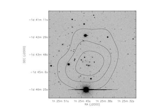
Figure 9: X–ray contours in the ROSAT hard band of source 13 in A194 field overlaid on a CCD R band image (15 min exposure at the CTIO 1.5 m).

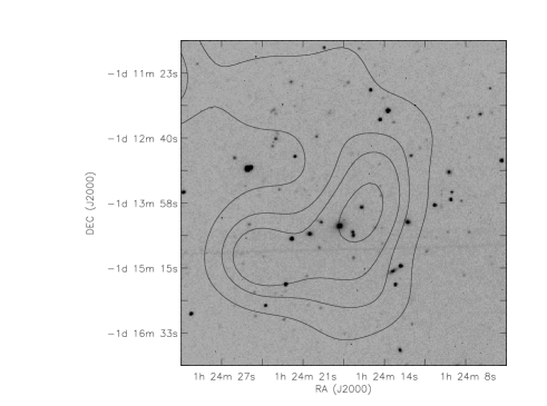
Figure 10: X–ray contours in the ROSAT hard band of source 20 in A194 field overlaid on a CCD I band image (15 min exposure at the CTIO 1.5 m).

For this purpose in Figure 7 the positions of the detected sources are overlaid on a $40^{\prime}\times 40^{\prime}$ DSS plate of the A1367 center: radii of circles are equal to the $3\,\sigma$ error boxes. No secure identifications with stars were found for the boresight correction so that we only used the bright elliptical galaxy displaced by $\sim 14^{\prime\prime}$ from the brightest X–ray source (1) (see Figure 7). This value has been adopted for the boresight correction and provides a good match also for the other sources (e.g. 8, 11, 13). Out of the 28 detected X–ray sources, 3 have galaxies members of the cluster within their error boxes (and possibly other 2, see Table 2) and 1 is a quasar (source 28). The identification of these galaxies with cluster members is further supported by the fact that their fluxes (calculated using a 2 keV bremsstrahlung spectrum and a $5\times 10^{20}$ cm^-2 column density) would convert into luminosities ranging from 0.6 to $6.6\times 10^{41}$ erg s^-1 at the cluster redshift. GAL presented several more identifications, but some appear to be inconsistent with the better positional accuracy obtained with our technique (see Table 2). We also find several extended sources (4, 5, 7, 10, 11, 14, 16 and 28, see Table 2). The extension of source 11 may be still contaminated by the cluster emission, being at its center, while source 28 is problematic (see note in Table 2). The classification of sources outside the PSPC rib however is less reliable.

4.2 A194

Abell 194 is a nearby ($z=0.018$) poor ($R=0$) cluster with little extended emission. The 16317 s ROSAT observation had not been previously analysed. The results are reported in Table 3. In Figure 8 the X–ray sources are overlaid on a $40^{\prime}\times 40^{\prime}$ DSS plate of the A194 center. In this case a boresight correction of $8^{\prime\prime}$ was applied, taking as a reference three Guide Star Catalog objects (source 2, 12 and 17 in Table 3). We detected 26 sources 4 of which are known galaxies of the cluster. In this case the expected number of background object is even lower (given the higher flux limit) than in the case of A1367.

The comparison of the source extension (FWHM) with the PSPC PSF allows us to detected 6 extended sources, namely 4, 11, 13, 20, 22 and 26 (see Table 3 and Figure 3). Two of these sources (12 and 26) are likely associated with galaxies members of the cluster. Follow-up CCD observations obtained at the CTIO 1.5 m telescope reveal a significant overdensity of galaxies around sources 13 and 20 (Figures 9 and 10). Thus, we believe that these sources are two newly discovered intermediate redshift galaxy clusters.

5 Summary

We have presented a new technique for a multi-scale analysis of astronomical X–ray images particularly suited for the detection and the characterisation of small and intermediate scale features embedded in a strongly varying background, such as the emission from clusters of galaxies. We have showed that even a rough subtraction of the extended component is needed in order to avoid positional biases in the detection thresholds. Our technique makes use of a 4-dimensional fit in the small and intermediate scale wavelet space which is first “decimated” to avoid redundancy and strong correlations. This approach leads to a better characterisation of the detected sources when compared with a 2-dimensional fit over the entire range of scales (e.g. GAL).

The application of this technique to two nearby cluster of galaxies has revealed a sizeable number of small-scale features which are thus believed to be a common property of nearby clusters. We detected 28 sources in the central part of A1367 (up to about $30^{\prime}$ from its center) and 26 in A194 ($28^{\prime}$ from its center). Since this surface density of sources significantly exceeds the value expected from the number counts in the field, we conclude that most of these sources are indeed physically bound to the cluster.

We provide a catalog of sources indicating (when possible) their likely optical identifications and those classified as extended. Two of the extended sources in A194 field are found to be associated with serendipitous background galaxy clusters expected to lie at intermediate redshifts.

- [1] Bechtold J., Forman W., Giacconi R., Jones C., Schwarz J., Tucker W., Van Speybroeck L., 1983, ApJ 265 26 (BAL)
- [2] Bijaoui A., Giudicelli M., 1992, Exp. Astr. 1 347
- [3] Bijaoui A. et al., 1995, Signal Processing 46 345
- [4] Campana S., Lazzati D., Tagliaferri G. et al., 1997, in preparation
- [5] Chincarini G., Giovannelli R., Haynes M., Fontanelli P., 1983, ApJ 267 511
- [6] Damiani F., Maggio A., Micela G., Sciortino S., 1997a, ApJ 483 350
- [7] Damiani F., Maggio A., Micela G., Sciortino S., 1997b, ApJ 483 370
- [8] Grebenev S.A., Forman W., Jones C., Murray S., 1995, ApJ 445 607 (GAL)
- [9] Farge M., 1992, Ann. Rev. Fluid Mech. 24 395
- [10] Hasinger G., Burg R., Giacconi R., Hartner G., Schmidt M., Trümper J., Zamorani G., 1993, A&A 275 1
- [11] Lazzati D., 1996, Degree Thesis, Università degli studi di Milano-Como
- [12] Lazzati D., Campana S., 1997, in preparation
- [13] Pando J., Fang L., 1996, ApJ 459 1
- [14] Pislar V., Durret F., Gerbal D., Lima Neto G.B., Slezak E., 1997, A&A 322 53
- [15] Plucinsky P.P., Snowden S.L., Briel U., Hasinger G., Pfeffermann E., 1993, ApJ 418 519
- [16] Rosati P., 1995, Ph.D. Thesis, Università “La Sapienza” di Roma
- [17] Rosati P., Della Ceca R., Burg R., Norman C., Giacconi R., 1995, ApJ 445 L11
- [18] Rue F., Bijaoui A., 1996, Vistas in Astronomy 40 495
- [19] Slezak E., Gerbal D., Durret F., 1995, AJ 108 1996
- [20] Snowden S.L., 1995, Cookbook for analysis procedures for ROSAT XRT/PSPC observations of extended objects and the diffuse background (Greenbelt, MD: Goddard Space Flight Center).
- [21] Snowden S.L., Freyberg M.J., 1993, ApJ 404 403
- [22] Snowden S.L., McCammon D., Burrows D.N., Mendenhall J.A., 1994, ApJ 424 714
- [23] Snowden S.L., Plucinsky P.P., Briel U., Hasinger G., Pfeffermann E., 1992, ApJ 393 819
- [24] Vikhlinin A., Forman W., Jones C., 1997, ApJ 474 L7