A standard stellar library for evolutionary synthesis

Abstract

A standard library of theoretical stellar spectra intended for multiple synthetic photometry applications including spectral evolutionary synthesis is presented. The grid includes M dwarf model spectra, hence complementing the first library version established in Paper I (Lejeune, Cuisinier & Buser 1997). It covers wide ranges of fundamental parameters: $T_{\mathrm{eff}}$ : 50,000 K $\sim$ 2000 K, $\log g$ : 5.5 $\sim$ -1.02, and [M/H] : +1.0 $\sim$ -5.0. A correction procedure is also applied to the theoretical spectra in order to provide color-calibrated flux distributions over a large domain of effective temperatures. For this purpose, empirical $T_{\mathrm{eff}}$–color calibrations are constructed between 11500 K and 2000 K, and semi-empirical calibrations for non-solar abundances ([M/H] = -3.5 to +1.0) are established. Model colors and bolometric corrections for both the original and the corrected spectra, synthesized in the $(UBV)_{J}(RI)_{C}JHKLL^{\prime}M$ system, are given for the full range of stellar parameters. We find that the corrected spectra provide a more realistic representation of empirical stellar colors, though the method employed is not completely adapted to the lowest temperature models. In particular the original differential colors of the grid implied by metallicity and/or luminosity changes are not preserved below 2500 K. Limitations of the correction method used are also discussed.

1 Introduction

Grids of theoretical stellar spectra providing models at low and high metallicities are indispensable for modelling the chemical evolution of the integrated light of stellar systems from theoretical isochrones used to describe the time-dependent stellar population. However, even the combined uses of available modern stellar libraries in evolutionary synthesis studies (e.g. Buzzoni 1989, Worthey 1994, Bressan et al. 1994) have been handicapped by intrinsic inhomogeneities and incompleteness. Furthermore, one of the most serious difficulties arises from the fact that the synthetic spectra and colors provided by most theoretical libraries still show large systematic discrepancies with calibrations based on spectroscopic and photometric observations. This is particularly true at low effective temperatures for which an accurate modelling of the stellar spectra requires important molecular opacity data which are not yet completely available. Ultimately, these limitations lead unavoidably to serious uncertainties in the interpretation of the population model.

In order to overcome these major shortcomings, we have undertaken the construction of a comprehensive combined library of realistic stellar flux distributions intended for population and evolutionary synthesis studies. A preliminary version of such a standard grid was presented in Lejeune et al. (1997, Paper I, referred to hereafter as LCB97), along with an algorithm developed for correction and calibration of the (theoretical) spectra. In this previous grid, M dwarf models, which are important for the determination of mass-to-light ratios in stellar populations, were missing. We present here a more comprehensive library which incorporates these dwarf spectra. The construction of this basic combined library is presented in the following section. The empirical $T_{\mathrm{eff}}$–color relations in UBVRIJHKL photometry, required to calibrate the spectra, are presented in section 3. Section 4 is dedicated to the correction of the theoretical spectra; in particular, we also examine the properties and the limitations of the method used when applied to the M dwarf models. Finally, we summarize the main properties of this new standard library in view of its synthetic photometry applications.

2 The model library

2.1 Construction of a combined library

Proceeding with the work undertaken in LCB97, we have built a more extensive library providing now almost complete coverage of the stellar parameter ranges in $T_{\mathrm{eff}}$, $\log g$, [M/H] which are required for population and evolutionary synthesis studies. This new grid is complementing the previous version by the addition of M dwarf model spectra. Different basic libraries have been assembled: the Kurucz (1995, [K95]) models provide wide coverage in $T_{\mathrm{eff}}$ (50,000 K $\sim$ 3500 K), $\log g$ (5.0 $\sim$ 0.0), and [M/H] (+1.0 $\sim$ -5.0), whereas in the temperature range 3500 K $\sim$ 2500 K the M giants spectra are represented by the hybrid “B+F” models constructed from spectra of Fluks et al. (1994) and Bessell et al. (1989, 1991 [BBSW]) (LCB97). For the M dwarf models, we introduced the synthetic spectra of cool stars originating from the Allard & Hauschildt (1995, [AH95]) grid. Thus, the previous library is extended by models within the following parameter ranges: 3500 K $>$ $T_{\mathrm{eff}}$ $\geq$ 2000 K, 5.5 $\geq$ $\log g$ $\geq$ 3.5 and +0.5 $\geq$ [M/H] $\geq$ -4.0. Fig. 1 gives a 3-D representation of the new combined library.

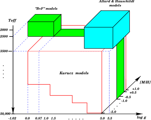
Figure 1: Coverage of the final combined library in the stellar parameter space. “B+F” models are those constructed for M giants from Fluks et al. and BBSW spectra (see LCB97).

The “base model grid” of AH95 atmosphere models (referred to hereafter as the “Extended” models) used here present several improvements compared to the previous generation models of Allard (1990). In particular, new molecular opacities have been incorporated and the opacity sampling technique has been introduced in order to improve the treatment of some of the atomic and molecular lines. For solar metallicity, we used an upgraded version (referred to as the “NextGen” models version) of the “base model grid”. In these new models a more extensive list of 12 million TiO lines (Jørgensen 1994) has also been included, with a more rigourous line-by-line treatment instead of the Just Overlapping Line Approximation (JOLA) previously used. The main effect is the reduction of the derived effective temperature by $\sim$ 150 K (Jones et al. 1996). We also found that these new models provide more realistic UBV colors than the previous generations (see Section 4.2). Because the “NextGen” model grid is still incomplete, only solar-abundance spectra can be included in order to cover the whole range of $T_{\mathrm{eff}}$ and $\log g$ provided by the hybrid library. For other metallicities, we still use the “Extended” models.

In the combined library, all the original spectra were rebinned on the same K95 wavelength grid, from 9.1 nm to 160 $\mu$m, with a mean resolution of $\sim$ 10 Å in the ultraviolet and $\sim$ 20 Å in the visible. Recall that the M giant model spectra “B+F” are metallicity-independent blueward of 4900 Å owing to the introduction of the Fluks et al. models in this spectral range, and that a black-body tail was attached for $\lambda\geq$ 4070 nm (see LCB97). The AH95 spectra stop at 20 $\mu$m, and for $\lambda$ $>$ 3 $\mu$m the resolution is not sufficient for an accurate description of the synthetic spectrum. In order to cover the whole K95 wavelength range, we then connected a black-body to the synthetic spectra beyond $\sim$ 5 $\mu$m (M band).

These model spectra – except for the updated NextGen models used in this work for solar metallicity – are available on a CD-ROM collecting various materials for galaxy evolution modelling (Leitherer et al. 1996), or by request on anonymous ftp, and have been used for single stellar populations models (Bruzual 1996, Bruzual et al. 1997, Lejeune 1997).

2.2 Model colors and bolometric corrections

Synthetic UBVRIJHKLL’M colors and bolometric corrections have also been computed from the theoretical stellar energy distributions (SEDs) over the whole range of parameters available in the grid, using the filter transmission functions given by Buser (1978) for $UBV$, Bessell (1979) for $(RI)_{C}$, and Bessell & Brett (1988) for $JHKLL^{\prime}M$. The zero-points were defined from the Vega model spectra of Kurucz (1991) by fitting to the observed values from Johnson (1966) (U-B = B-V = 0.0), Bessell & Brett (1988) (J-H = H-K = K-L = K-L’ = K-M = 0.0), and Bessell (1983) (V-I = 0.005, R-I = -0.004). For the bolometric corrections, we followed the zero-pointing procedure described in Buser & Kurucz (1978). We first (arbitrarily) set the smallest bolometric correction for the ($T_{\mathrm{eff}}$ = 7000 K, $\log g$ = 1.0) model to zero. This produces $BC^{\prime}_{\mathrm{V}}$ = -0.190 for the solar model, $T_{\mathrm{eff}}$ = 5777 K, $\log g$ = 4.44 (LCB97). The zero-point is then defined,

$$BC_{\mathrm{V}}=BC^{\prime}_{\mathrm{V}}+0.082\,,$$ (1)

in order for the present theoretical calculations to provide the best fit of the empirical bolometric-correction scale of Flower (1996). Adopting these definitions and the standard value of the solar radius (Allen 1973) we find $L=3.84510^{33}$ erg/s, $M_{\mathrm{V}}$ = 4.854 and $BC_{V}=-0.108$ for the solar model. Tables of theoretical colors and bolometric corrections for the whole range of stellar parameters in the grid are available in electronic form.

3 Temperature–color calibrations

3.1 Empirical calibrations at solar metallicity

In the correction procedure defined in LCB97, the empirical temperature–color calibrations are the basic links between the model colors and the observations. First, they provide a crucial point of comparison, and secondly, they are used to define the empirical and theoretical pseudo-continua from which the correction functions will be defined in the following. Over a large range of temperatures, we used the empirical $T_{\mathrm{eff}}$–$(UBV)_{J}(RI)_{C}JHKL$ relations discussed in detail in Paper I, but the inclusion of the M dwarf models in the library now leads us to extend the previous calibrations to the bottom of the main sequence. Observations of very low-mass stars being still rather fragmentary, the construction of these temperature–color relations require indirect empirical methods which are now described.

3.1.1 Dwarfs

Over the temperature range 11500 K $\geq$ $T_{\mathrm{eff}}$ $\geq$ 4250 K, the empirical temperature–color sequences are based upon the temperature scale of Schmidt-Kaler (1982) for U–B and Flower (1996) for B–V, and the two-color relations compiled in the literature (FitzGerald 1970, Bessell 1979, and Bessell & Brett 1988).

For $T_{\mathrm{eff}}$ $\leq$ 4000 K, the temperature scale is very controversial, in particular because of the difficulty to accurately model the complex featured M dwarf spectra. Due to the lack of very reliable model-atmospheres, indirect methods such as blackbody or gray-body fitting techniques have been used to estimate effective temperatures of the intrinsically faintest stars (Veeder 1974, Berriman & Reid 1987, Bessell 1991, Berriman, Reid & Leggett 1992, Tinney, Mould & Reid 1993). In practice, the temperatures derived from fitting to model spectra (e.g. Kirkpatrick et al. 1993, Jones et al. 1994) are systematically $\sim$ 300 K warmer than those estimated by empirical methods. Recently, a redetermination of the effective temperatures using the NextGen version of the AH95 model spectra has been proposed. Leggett et al. (1996) used observed infrared low-resolution spectra and photometry to compare with models. They found radii and effective temperatures which are consistent with estimates based only on photometric data. Their study shows that these updated models should provide, for the first time, a realistic temperature scale for M dwarfs. On the other hand, Jones et al. (1996), using a specific spectral region (1.16–1.22 $\mu$m) which is very sensitive to parameter changes of M dwarfs (Jones et al. 1994), have derived stellar parameters by fitting synthetic spectra for a limited sample of well-known low-mass stars. They found that the new models provide reasonable representations of the overall spectral features, with realistic relative strength variations induced by changes in stellar parameters.

Based on these promising – although preliminary – results of Leggett et al., providing closer agreement between theoretical and observational temperature scales, we adopted a mean relation constructed from a compilation of the results of Bessell (1991), Berriman et al. (1992), and Leggett et al. (1996). Fig. 2 shows the different effective temperature scales adopted by these authors, as a function of I–K and V–K. All the IR photometric data have been transformed to the homogeneous JHKL system of Bessell & Brett. The solid line is a polynomial fit derived from these data. For comparison, we have also added in the figure the $T_{\mathrm{eff}}$–values estimated by Jones et al. (1996) for 6 stars (large open symbols) having VIK photometry data given in Jones et al. (1994). Due to the limited spectral range used, the temperatures estimated by Jones et al. (1996) are still uncertain, and hence have not been used to define the mean relation given in Fig. 2. For stars cooler than 3000 K, the discrepancies between the different temperature scales appear slightly more pronounced in I–K than in V–K. For this reason, V–K was preferred to I–K for establishing the mean temperature scale of M dwarfs. We found:

$$V-K=1.18\>10^{-6}*(T_{\mathrm{eff}})^{2}-0.01*T_{\mathrm{eff}}+28.49\,.$$ (2)

For practical purposes, a good approximation of the inverse relation is given by:

$$T_{\mathrm{eff}}=18.27*(V-K)^{2}-504.88*(V-K)+5415\,.$$ (3)

Notice that this (V–K)–$T_{\mathrm{eff}}$ scale perfectly matches the Bessell (1991) calibration above 3000 K, and that the temperatures estimated by Leggett et al. are also in general agreement with this relation. The mean (V–K)–$T_{\mathrm{eff}}$ relation defined above was thus adopted as the basic scale for M dwarfs over the range 4000 K $\sim$ 2000 K.

For $T_{\mathrm{eff}}$ between 4000 K and 2600 K, we then used the $(BV)_{J}(RI)_{C}JHK$ photometric data given in Bessell (1991) and for stars hotter than $\sim$ 3000 K the U–B colors from FitzGerald (1970) in order to relate V–K to the other colors at a given temperature, via color–color transformations.

In order to establish the calibrations down to 2000 K, we used the two objects LHS2924 and GD165B with effective temperatures estimated by Jones et al. 1996 (2350 K and 2050 K, respectively), for which $VIJHKL$ photometry is given in Jones et al. (1994). The $T_{\mathrm{eff}}$ of LHS2924 was found to be in very good agreement with our temperature scale (Fig. 2) whereas GD165B is the coolest object with available infrared photometry. Therefore, the cool tails of our empirical calibrations for the J–H, J–K, H–K and K–L colors were required to match these two extreme points. Nevertheless, since these two objects are good brown dwarf candidates, with potentially non-solar abundances ([Fe/H] $\sim$ -0.5 for LHS2924 and +0.5 for GD165B, Jones et al. 1996), the empirical infrared stellar colors below 2300 K should be considered with caution. Furthermore, reliably accurate UBVRI photometry data for M dwarfs cooler than 3000 K (B-V $\sim$ 1.8) are also difficult to obtain – and are sparse indeed. Some relevant data can be found in the Gliese & Jahreiss (1991) catalog of nearby stars. Consequently, we extrapolated down to 2000 K the $T_{\mathrm{eff}}$–UBVRI calibrations defined above for hotter stars. Compared to the calibrations of Johnson (1966) and FitzGerald (1970), our (U–B)-(B–V) relation yields a better match of the extreme red points found in the Gliese & Jahreiss catalog (Fig. 3).

As before, the surface gravities along the dwarf sequence were defined at each $T_{\mathrm{eff}}$ from a ZAMS computed by the Bruzual & Charlot (1996, private communication) isochrone synthesis program.

Figure 2: A comparison of different temperature scales of M dwarfs adopted by several authors. The solid line is a polynomial fit performed on all the data, except those of Jones et al. 1996 (large open symbols). See text for explanations.

Figure 3: U–B/B–V empirical sequences compared to the Gliese & Jahreiss (1991, CSN3) catalog of nearby stars.

3.1.2 Giants

For cool giants, the Ridgway et al. (1980) (V–K)–$T_{\mathrm{eff}}$ relation was used as the basic temperature scale. As in Paper I, the different $T_{\mathrm{eff}}$–color sequences were constructed by compiling the photometric calibrations from Johnson (1966), Bessell (1979), Bessell & Brett (1988), and recent observations of M giants given by Fluks et al. (1994). A 1 $M_{\odot}$ evolutionary track (Schaller et al. 1992) was used to define the $\log g$ of the red giants with $T_{\mathrm{eff}}$ in the interval 4500 K $\sim$ 2500 K.

3.2 Semi-empirical calibrations for non-solar abundances

In LCB97, one of the basic assumptions made to define the correction process of the spectra is that the original model grids provide realistic color differences with respect to metal-content variations. These properties, established in particular for the K95 grid from Washington photometry by Lejeune & Buser (1996), can be naturally applied to define semi-empirical $T_{\mathrm{eff}}$–color calibrations at different metallicities. This is achieved by calculating at a given effective temperature the theoretical color differences due uniquely to a change in the chemical composition (hereafter called differential colors). These differences are then added to the colors provided by the empirical $T_{\mathrm{eff}}$–color calibrations for solar metallicity in order to fix the semi-empirical colors, $\stackrel{{\scriptstyle\sim}}{{c_{ij}}}^{emp}$, at a given metallicity:

$$\stackrel{{\scriptstyle\sim}}{{c_{ij}}}^{emp}\!\!\!\!(T,\log g_{\mathrm{seq}},[M/H])=c_{ij}^{emp}(T,\log g_{\mathrm{seq}},[M/H]\!=\!0)$$ (4)

$$+\Delta c_{ij}(T,\log g_{\mathrm{seq}},\Delta[M/H])\,,$$

where $\log g_{\mathrm{seq}}$ designates the surface gravity along the giant or the dwarf sequences, as defined by the empirical calibrations. The resulting empirical and semi-empirical $T_{\mathrm{eff}}$–color calibrations for the dwarfs and giants are given in Tables 1 to 10. Empirical colors for M dwarfs (2000 K $\sim$ 3500 K) are given in the range –3.5 $<$ [M/H] $<$ +0.5, while for M giants between 2500 K and 3500 K the calibrations are defined for –1.0 $<$ [M/H] $<$ +0.5. Theoretical bolometric corrections, $BC_{V}$ (see Eq. 1), are given as derived from the final grid of corrected spectra (see Section 4 and LCB97). While for completeness the semi-empirical calibrations are given for the largest possible ranges of colors and effective temperatures in Tables 1 to 10, we should emphasize here that the UBV magnitudes for the coolest M dwarf models – and hence the corresponding differential colors – are still rather uncertain, as will be shown in Section 4.2.

4 Calibration of theoretical spectra

4.1 Correction procedure and conservation of the original differential properties

The need to re-calibrate the theoretical SEDs was clearly demonstrated in the previous work, by comparing (i) the model colors obtained from the original synthetic spectra with the empirical temperature–color calibrations, and (ii) the model colors originating from the different basic libraries between themselves. In Fig. 6 of LCB97, discrepancies as large as $\sim$ 0.5 mag can be found for instance in U–B and B–V for $T_{\mathrm{eff}}$ $<$ 3500 K. A correction procedure was developed in order to provide color-calibrated theoretical fluxes over a large wavelength range, (typically from U to L), while preserving the color differences due to gravity and metallicity variations given by the different original grids. This method was based on the definition of correction functions at a given effective temperature, $\Phi_{\lambda}(T)$, obtained from the ratio of the corresponding empirical and theoretical pseudo-continua at each wavelength. The pseudo-continua in turn were calculated from the colors and, hence, the monochromatic fluxes within each wavelength band as black-bodies with smoothed color temperatures varying with wavelength, $T_{c}(\lambda)$:

$$pc_{\lambda}(T_{\mathrm{e}ff})\propto B_{\lambda}(T_{c}(\lambda)).$$ (5)

A corrected spectrum can therefore be simply computed by multiplying the original spectrum for a given set of stellar parameters ($T_{\mathrm{eff}}$, $\log g$, [M/H]) with the corresponding correction function at the same effective temperature. A scaling factor, $\xi(T,\log g,\chi)$, is finally applied to the corrected spectrum in order to conserve the bolometric flux (Eq. 9). As the correction function is, by definition, a factor which depends on the effective temperature only, this simple algorithm also preserves, to first order, the original differential grid properties implied by metallicity and/or surface gravity changes, and thus satisfies the basic requirement imposed on the correction procedure.

While this is true for the monochromatic magnitude differences – the correction function becomes an additive constant on a logarithmic scale –, this condition cannot be fully achieved for the (broad-band) colors, which represent heterochromatic measures of the flux. Yet, if we consider an original spectrum for a given set of stellar parameters, $S^{o}_{\lambda}(T,\log g_{1},\chi_{1})$, the magnitude $m_{i}$ in filter i is:

$$m_{i}^{o}(T,\log g_{1},\chi_{1})=$$ (6)

$$-2.5\log\int_{\lambda_{m_{i}}}^{\lambda_{M_{i}}}S^{o}_{\lambda}(T,\log g_{1},\chi_{1})P^{i}_{\lambda}\,d\lambda+K_{i}\,,$$

where $P^{i}_{\lambda}$ is the normalized transmission function of the filter $i$ defined between $\lambda_{m_{i}}$ and $\lambda_{M_{i}}$. For different values of the gravity and the chemical composition at the same $T_{\mathrm{eff}}$, we have

$$m_{i}^{o}(T,\log g_{2},\chi_{2})=$$ (7)

$$-2.5\log\int_{\lambda_{m_{i}}}^{\lambda_{M_{i}}}S^{o}_{\lambda}(T,\log g_{2},\chi_{2})P^{i}_{\lambda}\,d\lambda+K_{i}\,.$$

The color difference $\Delta c_{ij}^{o}$ due to the variations in $\log g$ and $\chi$ are then given by

$$\Delta c_{ij}^{o} =-2.5\log \left(\frac{\displaystyle\int_{\lambda_{m_{i}}}^{\lambda_{M_{i}}}S^{o}_{\lambda}(T,\log g_{1},\chi_{1})P^{i}_{\lambda}d\lambda}{\displaystyle\int_{\lambda_{m_{j}}}^{\lambda_{M_{j}}}S^{o}_{\lambda}(T,\log g_{1},\chi_{1})P^{j}_{\lambda}d\lambda}\right.$$ (8)

$$\times\left.\frac{\displaystyle\int_{\lambda_{m_{j}}}^{\lambda_{M_{j}}}S^{o}_{\lambda}(T,\log g_{2},\chi_{2})P^{j}_{\lambda}d\lambda}{\displaystyle\int_{\lambda_{m_{i}}}^{\lambda_{M_{i}}}S^{o}_{\lambda}(T,\log g_{2},\chi_{2})P^{i}_{\lambda}d\lambda}\right).$$

Since for the corrected spectra (LCB97),

$$S^{c}_{\lambda}(T,\log g,\chi)=\Phi_{\lambda}(T)\cdot\xi(T,\log g,\chi)\cdot S^{o}_{\lambda}(T,\log g,\chi),$$ (9)

we have, after elimination of $\xi$ in the color term:

$$\Delta c_{ij}^{c} =-2.5\log \left(\frac{\displaystyle\int_{\lambda_{m_{i}}}^{\lambda_{M_{i}}}\Phi_{\lambda}(T)\,S^{o}_{\lambda}(T,\log g_{1},\chi_{1})P^{i}_{\lambda}d\lambda}{\displaystyle\int_{\lambda_{m_{j}}}^{\lambda_{M_{j}}}\Phi_{\lambda}(T)\,S^{o}_{\lambda}(T,\log g_{1},\chi_{1})P^{j}_{\lambda}d\lambda}\right.$$ (10)

$$\!\!\times\left.\frac{\displaystyle\int_{\lambda_{m_{j}}}^{\lambda_{M_{j}}}\!\!\!\!\Phi_{\lambda}(T)\,S^{o}_{\lambda}(T,\log g_{2},\chi_{2})P^{j}_{\lambda}d\lambda}{\displaystyle\int_{\lambda_{m_{i}}}^{\lambda_{M_{i}}}\!\!\!\!\Phi_{\lambda}(T)\,S^{o}_{\lambda}(T,\log g_{2},\chi_{2})P^{i}_{\lambda}d\lambda}\right)\!\!.$$

Thus the differential colors are rigorously preserved by the correction procedure (i.e. $\Delta c_{ij}^{o}=\Delta c_{ij}^{c}$) if $\Phi_{\lambda}(T)$ is constant between $\lambda_{m}$ and $\lambda_{M}$. In practice, these rather severe constraints are well matched – and the corresponding $\delta(\Delta c_{ij})$ are small – if $\Phi_{\lambda}(T)$ varies slowly across the passbands or, equivalently, as long as the filters are not too wide.

Figs. 18 and 19 of LCB97 show, in fact, that the color residuals are negligible over the whole ranges of UBVRIJHKL colors and model parameters. Significant residuals ($\sim$ 0.05 mag) are found in R–I at the lowest temperatures because of the more significant variations of the correction functions inside the long-tailed R filter.

4.2 Correction of M dwarf model spectra

In Fig. 4, we compare a sequence of theoretical colors computed from the dwarf model SEDs to the empirical colors. While the hottest models (K95) match quite well the observed sequences – except for $T_{\mathrm{eff}}$ $<$ 4000 $\sim$ 3750 K – the coolest ones (AH95) exhibit more serious discrepancies, in particular in the blue-optical colors. The Extended models (open squares) provide unrealistic U–B and B–V colors, differing by as much as 2 $\sim$ 3 mag relative to the NextGen version models (crosses). At longer wavelengths, both these new and old M dwarf model generations seem more realistic, although the infrared colors appear systematically too blue probably due to an incomplete $H_{2}O$ opacity list at solar-metallicity used in the calculations (Allard, private communication).

Figure 4: Colors of original models of dwarfs compared to our empirical $T_{\mathrm{eff}}$–color relations (solid lines). The “Extended” models (open squares) exhibit larger deviations (except in H–K) and unrealistic U–B and B–V colors compared to the “NextGen” (labelled “NG”) models (crosses).

In order to provide more realistic (broad-band) colors for M dwarfs, we have applied the correction method described in Section 4.1, using the pseudo-continua calculated from the updated empirical temperature–color relationships between 2000 K and 11500 K. However, in the range 2000 K $\sim$ 4500 K we have to distinguish between the “dwarf” and the “giant” correction functions derived from model spectra originating from different grids (AH95 and “B+F”, respectively). This was done by fixing the lower limit of $\log g$ for a “dwarf” model to 3.0 dex. Thus, all the spectra with $\log g$ lower than 3.0 and $T_{\mathrm{eff}}$ less than 4500 K are corrected according to the giant empirical color sequences, while the others are calibrated from the dwarf sequences. For [M/H] = 0, we also defined corrections functions to be applied uniquely to the NextGen models, independently of those computed for the Extended models used at other metallicities. In Fig. 5 we compare the corrected model colors to the $T_{\mathrm{eff}}$–color calibrations: most of the theoretical colors now match very well the empirical relations. For the largest original deviations found in U–B and B–V below 3000 K, important discrepancies still remain (more than 1 mag for the Extended models), but the corrected colors should nevertheless provide more reliable values, in particular those predicted by the NextGen models.

As for the original model spectra, UBVRIJHKLM corrected model colors and bolometric corrections have been synthetised for the whole range of parameters provided by the complete library. Color grids are given in electronic tables accompanying this paper.

Figure 5: Same as Fig. 4 but for the corrected models. The corrections provide a perfect match of the empirical colors over the whole range of $T_{\mathrm{eff}}$, except in U–B and B–V below 2500 K, where significant discrepancies persist.

Because the corrections are so substantial, the question which naturally arises is how well preserved are the original differential colors for the coolest M dwarfs. We have computed, for these models, the residual color differences between corrected and original model colors, $\delta(\Delta c_{ij})=(\Delta c_{ij}^{c}-\Delta c_{ij}^{o})$. For metal-content variations the results are presented in Fig. 6, where $\delta(\Delta c_{ij})$ is plotted as a function of [M/H]. At low temperatures ($<$ 2200 K) and low metallicities ($<$ -2.0), differences as large as $\sim$ 2 mag are reached for U–B and B–V ! For the other colors the residuals are smaller, but typical values of order $\sim$ 0.2 mag still remain for the coolest and the most metal-deficient models. Clearly, the original grid properties are not conserved for these models.

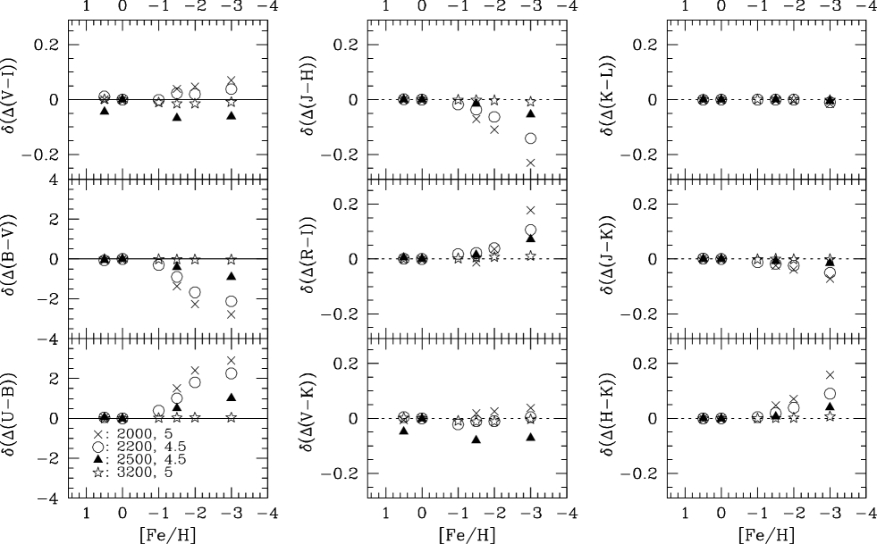
Figure 6: Color–difference residuals between corrected and original models as functions of [Fe/H] for some of the M dwarf models. The symbols indicate the difference between the color excess of a corrected model at a given metallicity and the color excess of the corresponding original model, having the same $T_{\mathrm{eff}}$ and $\log g$ (as indicated on the bottom–left panel). The color excesses are calculated as: $\Delta c_{ij}=c_{ij}(\chi)-c_{ij}(\chi_{\odot})$

The main reason behind these deviations is the strong variation of the correction factors within the spectral range covered by broad-band filters, as discussed in Section 4.1. Fig. 7 shows the correction functions computed for some of the coolest models, compared to the respective positions of the different passbands, and their effect on a cool dwarf model spectrum (bottom panel). As previously, the functions are all normalized at 817 nm in the I band (LCB97) and plotted on a logarithmic scale in order to emphasize the relative differences. As we can see for 2000 K (solid line) and 2500 K (short-dashed line), the correction functions vary considerably across the UBV filters; e.g., the 2000 K–function changes by a factor $\sim$ 1000 between 400 and 600 nm ! These steep gradients inevitably degrade the resulting differential colors. Significant fluctuations of correction factors are also present in the JHK bands, accounting for the significant residuals seen in these differential colors. For the giants at 2500 K (thick line), the largest fluctuations appear in R and I, leading to the deviations found in LCB97 ($\sim$ 0.05) at this temperature.

Figure 7: Top panel. The correction functions applied to the M star models: for dwarf spectrum at 2000 K (thin solid line), 2500 K (long-dashed line), 3500 K (short-dashed line), and for giant spectrum at 2500 K (thick solid line). The different filters are also shown. Note the strong variations of these functions in the UBV bands for the coolest dwarf models (2000 K and 2500 K) which affect the differential colors.
Bottom panel. A corrected M dwarf spectrum (solid line) compared to the original one (dotted-line). An arbitrary shift has been applied for clarity.

4.3 Shortcomings of the correction algorithm

In order to investigate correction methods which better preserve the differential properties, we developed a procedure which avoids the use of functions applied to the spectra as multiplicative factors. This was done by introducing directly, as an input to the correction algorithm, the color differences, $\Delta c_{ij}(T,\Delta\log g,\Delta\chi)$, that we want to preserve from the original models. Generalizing the definitions of the non-solar $T_{\mathrm{eff}}$–color calibrations (Eq. 4), we define the semi-empirical colors of each model in the grid, $\stackrel{{\scriptstyle\sim}}{{c_{ij}}}(T,\log g,\chi)$, by adding to the empirical colors given in Table 1 the theoretical color differences due to changes in metallicity,$\Delta\chi$, and surface gravity, $\Delta\log g$:

$$\stackrel{{\scriptstyle\sim}}{{c_{ij}}}(T,\log g,\chi) = c_{ij}^{emp}(T,\log g_{\mathrm{seq}},\chi_{\odot})$$ (11)

$$+ \Delta c_{ij}(T,\Delta\log g,\Delta\chi)\,.$$

These semi-empirical colors then define the semi-empirical pseudo-continuum, $\stackrel{{\scriptstyle\sim}}{{pc}}_{\lambda}(T,\log g,\chi)$, at a given parameter set in the grid, following the method described in Paper I. In order to preserve the detailed information at the resolution of the synthetic spectra, a “spectral function”, $\Gamma_{\lambda}(T,\log g,\chi)$, obtained by the ratio of the original model spectrum to the theoretical pseudo-continuum, is then multiplied with the semi-empirical pseudo continuum, in order to define the corrected spectra (see Appendix):

$$S^{c}_{\lambda}(T,\log g,\chi)=\stackrel{{\scriptstyle\sim}}{{pc}}_{\lambda}(T,\log g,\chi)*\Gamma_{\lambda}(T,\log g,\chi)\,.$$ (12)

This “differential correction” method should naturally preserve the original spectral features and the color differences of the models.

Identical tests as those performed in Section 4.2 for measuring the differential corrected colors indicate that, unfortunately, this “differential correction” algorithm fails to provide significant improvements over the conservation of differential colors attempted via the previous method. For models hotter than 3000 K, the residuals are still negligible ($<$ 0.02 mag) and the two methods are really equivalent, but in the coolest dwarf regime, the new algorithm gives even worse results for UBV colors.

Thus, none of the two correction methods are able to preserve the differential color properties for the coolest star models to within the desired accuracy. Clearly, the definition and use of a pseudo-continuum is inadequate for such stars. Indeed, at these low temperatures, the presence of large and strong molecular absorption bands complicates the stellar spectra and hence also affects significantly the (broad-band) colors. Therefore, a pseudo-continuum defined from these colors as a smoothed (black-body) function cannot trace the flux distribution accurately enough. As an illustration, the theoretical spectra and their derived pseudo-continua are compared in Fig. 8 for two low values of the effective temperature: for $T_{\mathrm{eff}}$ = 3500 K (left panel), the pseudo-continuum (normalized in the K band) follows the flux variations quite accurately, whereas for 2200 K (right panel), the spectrum is too complex to be described by a continuous function such as a pseudo-continuum. Therefore, for temperatures less than $\sim$ 2500 K, a correction function defined from smoothed energy distributions is not suitable for color-calibrating theoretical spectra. In the future, a more reliable calibration and correction method for these complicated spectra of the coolest stars must obviously be based on the higher–resolution, more detailed observed flux distributions provided by eight–color narrow-band photometry (White & Wing 1978) or by spectrophotometric data (e.g. Kirkpatrick et al. 1991; 1993).

Figure 8: Comparison of theoretical spectra and their derived pseudo-continua for two values of $T_{\mathrm{eff}}$. The points indicate the monochromatic fluxes given by the theoretical colors.

5 Conclusion

We have constructed a comprehensive library of theoretical stellar energy distributions from a combination of different basic grids of blanketed model atmosphere spectra. This new grid complements the preliminary version described in LCB97 by extending it to the M dwarfs models of Allard & Hauschildt (1995). It provides synthetic stellar spectra with useful resolution on a homogeneous wavelength grid, from 9.1 nm to 160 $\mu$m, over large ranges of fundamental parameters. This standard library should therefore be particularly suitable for spectral evolutionary synthesis studies of stellar systems and other synthetic photometry applications.

Comparison of synthetic photometry with empirical $T_{\mathrm{eff}}$–color sequences, established for the first time down to 2000 K, have shown important discrepancies for the coolest dwarf models. The correction procedure designed in the previous paper to provide color-calibrated fluxes has been extended and applied to the original dwarf spectra in the range 4500 K to 2000 K. Although this seems to result in more realistic colors, the method induces significant changes in the original differential color properties. This stems from too strongly variable correction functions at low temperatures, resulting from the fact that the pseudo-continuum cannot be adequately defined for these stars. The empirical colors for dwarfs below 2500 K remain uncertain due to the lack of reliable observations. At the lowest temperatures, the corrected models should therefore be used with caution.

Despite these limitations, we expect that the corrected spectra provide at present a valuable option for deriving realistic stellar colors over extensive ranges of temperatures, luminosities, and metallicities which are required for reliable population synthesis modelling. Grids of model spectra and (UBVRIJHKLM) colors for both the original and the corrected versions of the present stellar library, as well as the semi-empirical calibrations presented in Tables 1 to 10, are fully available by electronic form at the Strasbourg data center (CDS).

Appendix

We give here a more detailed description of the differential correction algorithm discussed in Section 4.3.

For each model spectrum and given parameter values $(T,\log g,\chi)$ in the grid, we proceed along the following steps:

1. we compute the synthetic colors, $c_{ij}^{o}(T,\log g,\chi)$, from the original theoretical energy distribution, $S^{o}_{\lambda}(T,\log g,\chi)$, and the normalized response functions of the filters, $P^{i}_{\lambda}$, (Eq. 6) by

   $$c_{ij}^{o}(T,\log g,\chi)=$$ (13)

   $$-2.5\log\left(\frac{\displaystyle\int_{\lambda_{m_{i}}}^{\lambda_{M_{i}}}S^{o}_{\lambda}(T,\log g,\chi)P^{i}_{\lambda}d\lambda}{\displaystyle\int_{\lambda_{m_{j}}}^{\lambda_{M_{j}}}S^{o}_{\lambda}(T,\log g,\chi)P^{j}_{\lambda}d\lambda}\right)\,;$$

2. as described in detail in LCB97, these theoretical colors, and hence the monochromatic fluxes within each wavelength band, are then used to calculate the theoretical pseudo-continuum, ${pc}^{o}_{\lambda}(T,\log g,\chi)$, as a black-body with smoothed color temperatures, $T_{c}(\lambda)$, varying with wavelength:

   $${pc}^{o}_{\lambda}(T,\log g,\chi)\propto B_{\lambda}(T_{c}(\lambda))\,;$$ (14)

3. from the theoretical colors, $c_{ij}^{o}(T,\log g,\chi)$, we compute the theoretical color differences,

   $$\Delta c_{ij}(T,\Delta\log g,\Delta\chi)=$$ (15)

   $$c_{ij}^{o}(T,\log g,\chi)-c_{ij}^{o}(T,\log g_{\mathrm{seq}},\chi_{\odot})\,,$$

   where $\Delta\log g$ and $\Delta\chi$ are respectively the surface gravity and the metallicity variations relative to the empirical sequences – for dwarfs and giants at solar metallicity – given in Table 1:

   $$\Delta\log g=\log g-\log g_{\mathrm{seq}}\,,$$ (16)

   with

   $$\log g_{\mathrm{seq}}=\left\{\begin{array}[]{ll}\log g_{\,\mathrm{giant}}&\mbox{if $\log g<$ 3.0 and $T\leq$ 4500 K}\\ \log g_{\,\mathrm{dwarf}}&\mbox{otherwise}\,,\end{array}\right.$$

   and

   $$\Delta\chi=\chi-\chi_{\odot}\,;$$

4. by adding these color differences to the empirical colors, $c_{ij}^{emp}(T,\log g_{\mathrm{seq}},\chi_{\odot})$ given in Table 1, we then define the semi-empirical colors, $\stackrel{{\scriptstyle\sim}}{{c_{ij}}}(T,\log g,\chi)$:

   $$\stackrel{{\scriptstyle\sim}}{{c_{ij}}}(T,\log g,\chi) = c_{ij}^{emp}(T,\log g_{\mathrm{seq}},\chi_{\odot})$$ (17)

   $$+ \Delta c_{ij}(T,\Delta\log g,\Delta\chi)\,;$$

5. from Eq. (14), these semi-empirical colors allow us to calculate the semi-empirical pseudo-continuum, $\stackrel{{\scriptstyle\sim}}{{pc}}_{\lambda}(T,\log g,\chi)$;

6. a “spectral function”, $\Gamma_{\lambda}(T,\log g,\chi)$, which contains the high–resolution information of the theoretical spectrum, is defined by the ratio of the original spectrum and the theoretical pseudo-continuum,

   $$\Gamma_{\lambda}(T,\log g,\chi)=S^{o}_{\lambda}(T,\log g,\chi)\>/\>pc_{\lambda}(T,\log g,\chi)\,;$$ (18)

7. the corrected spectrum is finally computed by multiplying the spectral function with the semi-empirical pseudo–continuum:

   $$S^{c}_{\lambda}(T,\log g,\chi)=\stackrel{{\scriptstyle\sim}}{{pc}}_{\lambda}(T,\log g,\chi)*\Gamma_{\lambda}(T,\log g,\chi)\,.$$ (19)

Table 1: Adopted $T_{\mathrm{eff}}$–color relations and $\log g$ values for dwarfs and cool giants with [M/H] = 0.0

$T_{\mathrm{eff}}$	U-B	B-V	V-I	V-K	R-I	J-H	H-K	J-K	K-L	$BC_{\mathrm{V}}$	$\log g$
Dwarfs
2000.	3.119	2.664	6.148	11.090	2.921	1.192	0.682	1.874	0.891	-7.623	5.490
2200.	2.772	2.498	5.504	9.871	2.691	0.881	0.592	1.473	0.652	-6.496	5.417
2500.	2.253	2.249	4.558	8.214	2.365	0.711	0.431	1.142	0.403	-5.072	5.307
2800.	1.732	2.001	3.748	6.768	2.056	0.638	0.358	0.996	0.329	-3.836	5.199
3000.	1.418	1.820	3.242	5.918	1.842	0.616	0.315	0.931	0.273	-3.112	5.137
3200.	1.203	1.639	2.788	5.163	1.590	0.621	0.262	0.882	0.224	-2.468	5.052
3350.	1.067	1.550	2.481	4.668	1.377	0.639	0.231	0.870	0.201	-2.042	4.992
3500.	1.090	1.520	2.160	4.110	1.160	0.660	0.200	0.860	0.160	-1.632	4.900
3750.	1.209	1.448	1.854	3.714	0.947	0.664	0.171	0.835	0.142	-1.300	4.764
4000.	1.266	1.375	1.643	3.253	0.800	0.666	0.138	0.804	0.115	-0.975	4.672
4250.	1.200	1.294	1.371	2.953	0.656	0.626	0.116	0.742	0.103	-0.755	4.668
4500.	1.092	1.190	1.188	2.721	0.551	0.590	0.107	0.697	0.095	-0.595	4.653
4750.	0.907	1.049	0.998	2.412	0.458	0.536	0.098	0.634	0.079	-0.413	4.621
5000.	0.662	0.922	0.902	2.138	0.420	0.486	0.085	0.571	0.067	-0.292	4.598
5250.	0.442	0.812	0.846	1.960	0.397	0.455	0.075	0.530	0.060	-0.231	4.577
5500.	0.268	0.720	0.787	1.754	0.374	0.400	0.066	0.466	0.057	-0.174	4.549
5750.	0.115	0.640	0.707	1.550	0.342	0.347	0.053	0.400	0.053	-0.124	4.509
6000.	0.041	0.571	0.633	1.420	0.307	0.311	0.051	0.362	0.050	-0.094	4.462
6250.	0.008	0.508	0.565	1.239	0.274	0.266	0.045	0.311	0.045	-0.056	4.411
6500.	-0.016	0.449	0.501	1.058	0.244	0.219	0.039	0.258	0.039	-0.027	4.361
6750.	-0.010	0.394	0.448	0.896	0.221	0.175	0.036	0.211	0.037	-0.005	4.319
7000.	-0.013	0.343	0.384	0.771	0.193	0.144	0.033	0.177	0.036	0.005	4.295
7250.	0.049	0.293	0.320	0.684	0.163	0.127	0.029	0.156	0.035	0.023	4.287
7500.	0.097	0.247	0.289	0.607	0.150	0.110	0.027	0.137	0.032	0.029	4.288
7750.	0.094	0.203	0.267	0.532	0.140	0.092	0.026	0.118	0.031	0.015	4.292
8000.	0.097	0.162	0.211	0.449	0.113	0.076	0.021	0.097	0.026	0.003	4.295
8250.	0.090	0.126	0.144	0.364	0.078	0.062	0.014	0.076	0.019	-0.017	4.296
8500.	0.089	0.094	0.113	0.286	0.061	0.046	0.010	0.056	0.015	-0.041	4.296
8750.	0.076	0.067	0.097	0.208	0.053	0.028	0.008	0.036	0.013	-0.071	4.296
9000.	0.048	0.042	0.066	0.132	0.037	0.013	0.005	0.018	0.009	-0.108	4.297
9250.	0.019	0.021	0.011	0.069	0.006	0.007	0.003	0.010	0.005	-0.149	4.302
9500.	0.001	0.002	-0.018	0.005	-0.011	0.001	0.000	0.001	0.000	-0.185	4.307
9750.	-0.020	-0.014	-0.034	-0.047	-0.020	-0.006	-0.003	-0.009	-0.003	-0.222	4.300
10000.	-0.064	-0.029	-0.044	-0.085	-0.026	-0.013	-0.006	-0.019	-0.006	-0.279	4.275
10500.	-0.157	-0.055	-0.055	-0.144	-0.032	-0.023	-0.014	-0.037	-0.012	-0.406	4.208
11000.	-0.239	-0.076	-0.065	-0.210	-0.038	-0.034	-0.022	-0.056	-0.018	-0.534	4.182
11500.	-0.340	-0.094	-0.076	-0.286	-0.044	-0.046	-0.029	-0.075	-0.025	-0.723	4.190
Giants
2500.	-0.328	1.510	4.593	9.560	2.567	1.030	0.450	1.480	0.280	-6.246	-1.020
2800.	-0.005	1.509	4.320	8.995	2.535	1.015	0.424	1.446	0.276	-5.756	-0.774
3000.	0.285	1.510	4.060	8.458	2.495	1.001	0.391	1.399	0.257	-5.343	-0.320
3200.	0.876	1.508	3.468	7.232	2.264	0.984	0.359	1.340	0.230	-4.241	0.102
3350.	1.266	1.572	3.014	6.292	2.005	0.961	0.314	1.270	0.210	-3.368	0.415
3500.	1.557	1.593	2.625	5.487	1.755	0.942	0.258	1.195	0.188	-2.688	0.712
3750.	1.817	1.545	2.008	4.228	1.028	0.864	0.212	1.071	0.144	-1.586	1.174
4000.	1.668	1.417	1.574	3.475	0.735	0.768	0.157	0.923	0.118	-1.037	1.630
4250.	1.393	1.278	1.355	2.992	0.600	0.679	0.140	0.818	0.100	-0.731	2.127
4500.	1.118	1.140	1.127	2.613	0.510	0.609	0.107	0.714	0.086	-0.544	2.638

Table 2: Same as Table 1 for [M/H] = +1.0

$T_{\mathrm{eff}}$	U-B	B-V	V-I	V-K	R-I	J-H	H-K	J-K	K-L	$BC_{\mathrm{V}}$	$\log g$
Dwarfs
3500.	0.845	1.190	2.272	4.774	1.363	0.716	0.150	0.865	0.121	-2.157	4.900
3750.	1.142	1.178	1.906	4.323	1.135	0.724	0.115	0.839	0.087	-1.746	4.760
4000.	1.360	1.277	1.636	3.536	0.901	0.647	0.115	0.762	0.094	-1.161	4.670
4250.	1.419	1.331	1.392	3.070	0.709	0.568	0.114	0.682	0.107	-0.840	4.670
4500.	1.456	1.311	1.252	2.790	0.578	0.528	0.111	0.639	0.106	-0.655	4.650
4750.	1.359	1.201	1.081	2.463	0.470	0.476	0.102	0.578	0.088	-0.460	4.620
5000.	1.120	1.077	0.982	2.172	0.422	0.424	0.088	0.512	0.074	-0.322	4.600
5250.	0.887	0.964	0.915	1.976	0.392	0.391	0.077	0.469	0.064	-0.241	4.580
5500.	0.699	0.870	0.846	1.753	0.364	0.337	0.067	0.404	0.058	-0.164	4.550
5750.	0.523	0.784	0.759	1.534	0.329	0.287	0.052	0.340	0.049	-0.095	4.510
6000.	0.416	0.708	0.678	1.392	0.294	0.256	0.051	0.306	0.042	-0.050	4.460
6250.	0.343	0.637	0.602	1.201	0.260	0.216	0.045	0.261	0.033	0.001	4.410
6500.	0.274	0.571	0.528	1.012	0.227	0.173	0.040	0.213	0.025	0.043	4.360
6750.	0.231	0.505	0.467	0.844	0.203	0.133	0.038	0.171	0.024	0.071	4.320
7000.	0.183	0.442	0.396	0.716	0.175	0.107	0.035	0.142	0.024	0.086	4.300
7250.	0.208	0.379	0.327	0.629	0.144	0.095	0.030	0.125	0.025	0.102	4.290
7500.	0.231	0.319	0.290	0.551	0.129	0.083	0.027	0.109	0.022	0.104	4.290
7750.	0.208	0.264	0.264	0.476	0.119	0.067	0.025	0.093	0.023	0.089	4.290
8000.	0.196	0.212	0.204	0.393	0.091	0.055	0.020	0.073	0.019	0.078	4.300
8250.	0.168	0.167	0.140	0.314	0.059	0.045	0.012	0.057	0.014	0.057	4.300
8500.	0.142	0.129	0.111	0.242	0.045	0.032	0.007	0.039	0.008	0.030	4.300
8750.	0.109	0.096	0.097	0.168	0.038	0.016	0.004	0.021	0.004	0.000	4.300
9000.	0.069	0.062	0.064	0.091	0.023	0.003	0.000	0.003	0.000	-0.036	4.300
9250.	0.029	0.033	0.007	0.028	-0.008	-0.002	-0.003	-0.005	-0.004	-0.073	4.300
9500.	0.002	0.005	-0.024	-0.037	-0.025	-0.007	-0.006	-0.013	-0.008	-0.108	4.310
9750.	-0.026	-0.018	-0.042	-0.090	-0.034	-0.014	-0.009	-0.023	-0.010	-0.146	4.300
10000.	-0.074	-0.037	-0.052	-0.128	-0.039	-0.020	-0.012	-0.033	-0.013	-0.201	4.280
10500.	-0.169	-0.070	-0.065	-0.190	-0.046	-0.031	-0.020	-0.051	-0.019	-0.321	4.210
11000.	-0.253	-0.096	-0.076	-0.257	-0.052	-0.042	-0.029	-0.071	-0.026	-0.442	4.180
11500.	-0.357	-0.116	-0.088	-0.335	-0.058	-0.055	-0.036	-0.093	-0.034	-0.612	4.190
Giants
3500.	1.484	1.492	2.723	5.848	1.938	0.679	0.338	1.012	0.216	-3.061	0.710
3750.	1.999	1.591	2.049	4.394	1.133	0.643	0.276	0.914	0.169	-1.760	1.170
4000.	2.124	1.560	1.633	3.569	0.792	0.595	0.206	0.799	0.138	-1.139	1.630
4250.	2.044	1.467	1.438	3.060	0.630	0.545	0.174	0.718	0.117	-0.808	2.130
4500.	1.796	1.338	1.215	2.665	0.524	0.501	0.128	0.627	0.100	-0.607	2.640

Table 3: Same as Table 1 for [M/H] = +0.5

$T_{\mathrm{eff}}$	U-B	B-V	V-I	V-K	R-I	J-H	H-K	J-K	K-L	$BC_{\mathrm{V}}$	$\log g$
Dwarfs
2000.	3.161	2.358	6.437	11.492	2.922	1.168	0.775	1.943	0.821	-7.720	5.490
2200.	2.898	2.653	5.348	9.643	2.580	0.851	0.660	1.512	0.631	-6.157	5.420
2500.	2.328	2.328	4.348	8.033	2.241	0.672	0.463	1.136	0.412	-4.897	5.310
2800.	1.721	1.926	3.621	6.798	1.972	0.593	0.364	0.958	0.332	-4.039	5.200
3000.	1.420	1.852	3.075	5.896	1.709	0.585	0.320	0.905	0.286	-3.136	5.140
3200.	1.164	1.617	2.715	5.313	1.517	0.622	0.246	0.867	0.219	-2.632	5.050
3350.	0.994	1.463	2.540	5.044	1.392	0.664	0.203	0.866	0.183	-2.391	4.990
3500.	0.973	1.354	2.198	4.373	1.260	0.672	0.180	0.853	0.146	-1.836	4.900
3750.	1.208	1.331	1.865	3.978	1.030	0.712	0.139	0.850	0.109	-1.482	4.760
4000.	1.360	1.332	1.641	3.405	0.845	0.685	0.119	0.804	0.095	-1.066	4.670
4250.	1.346	1.316	1.390	3.018	0.679	0.615	0.111	0.726	0.100	-0.798	4.670
4500.	1.290	1.249	1.224	2.759	0.562	0.572	0.106	0.678	0.097	-0.626	4.650
4750.	1.121	1.117	1.036	2.439	0.461	0.517	0.097	0.614	0.080	-0.434	4.620
5000.	0.871	0.989	0.935	2.155	0.418	0.465	0.085	0.550	0.068	-0.303	4.600
5250.	0.649	0.877	0.871	1.968	0.391	0.433	0.074	0.507	0.059	-0.231	4.580
5500.	0.470	0.785	0.807	1.753	0.366	0.379	0.065	0.444	0.055	-0.163	4.550
5750.	0.305	0.703	0.723	1.542	0.333	0.326	0.051	0.379	0.048	-0.104	4.510
6000.	0.213	0.631	0.644	1.405	0.297	0.292	0.050	0.341	0.043	-0.066	4.460
6250.	0.159	0.564	0.572	1.218	0.264	0.247	0.045	0.292	0.038	-0.022	4.410
6500.	0.110	0.503	0.505	1.033	0.233	0.201	0.039	0.241	0.032	0.013	4.360
6750.	0.093	0.442	0.449	0.868	0.210	0.158	0.037	0.195	0.031	0.038	4.320
7000.	0.070	0.385	0.383	0.741	0.183	0.128	0.034	0.162	0.031	0.050	4.300
7250.	0.117	0.328	0.317	0.654	0.153	0.114	0.029	0.143	0.031	0.065	4.290
7500.	0.156	0.275	0.284	0.577	0.139	0.098	0.026	0.125	0.027	0.069	4.290
7750.	0.142	0.226	0.261	0.503	0.129	0.081	0.025	0.107	0.028	0.054	4.290
8000.	0.144	0.179	0.201	0.416	0.101	0.067	0.019	0.085	0.022	0.043	4.300
8250.	0.127	0.140	0.136	0.334	0.067	0.054	0.012	0.066	0.017	0.024	4.300
8500.	0.114	0.106	0.106	0.258	0.052	0.039	0.007	0.047	0.013	-0.002	4.300
8750.	0.089	0.076	0.092	0.184	0.045	0.022	0.005	0.028	0.009	-0.032	4.300
9000.	0.054	0.047	0.061	0.107	0.030	0.008	0.001	0.010	0.006	-0.069	4.300
9250.	0.018	0.023	0.005	0.045	-0.001	0.003	-0.001	0.002	0.002	-0.109	4.300
9500.	-0.003	0.001	-0.023	-0.018	-0.017	-0.002	-0.004	-0.006	-0.003	-0.146	4.310
9750.	-0.026	-0.018	-0.040	-0.069	-0.027	-0.009	-0.007	-0.016	-0.006	-0.185	4.300
10000.	-0.071	-0.034	-0.049	-0.107	-0.032	-0.016	-0.010	-0.026	-0.009	-0.242	4.280
10500.	-0.163	-0.062	-0.062	-0.168	-0.038	-0.027	-0.018	-0.044	-0.015	-0.366	4.210
11000.	-0.245	-0.084	-0.072	-0.234	-0.045	-0.037	-0.026	-0.064	-0.021	-0.491	4.180
11500.	-0.348	-0.103	-0.084	-0.312	-0.051	-0.050	-0.033	-0.084	-0.029	-0.671	4.190
Giants
2500.	-0.328	1.509	4.584	9.946	2.572	1.115	0.542	1.657	0.294	-6.517	-1.020
2800.	-0.005	1.508	4.273	9.470	2.529	1.008	0.503	1.519	0.298	-6.144	-0.770
3000.	0.285	1.509	3.900	8.956	2.442	0.938	0.460	1.405	0.284	-5.787	-0.320
3200.	0.876	1.501	3.529	7.822	2.295	0.888	0.406	1.290	0.220	-4.806	0.100
3350.	1.265	1.578	3.437	6.899	2.208	0.861	0.354	1.210	0.212	-3.975	0.410
3500.	1.563	1.543	2.661	5.648	1.843	0.801	0.321	1.117	0.199	-2.846	0.710
3750.	1.968	1.573	2.021	4.298	1.070	0.755	0.259	1.009	0.153	-1.653	1.170
4000.	1.964	1.493	1.602	3.518	0.754	0.691	0.189	0.878	0.125	-1.077	1.630
4250.	1.747	1.371	1.391	3.025	0.606	0.624	0.160	0.783	0.105	-0.762	2.130
4500.	1.442	1.232	1.163	2.638	0.510	0.567	0.118	0.682	0.090	-0.568	2.640

Table 4: Same as Table 1 for [M/H] = -0.5

$T_{\mathrm{eff}}$	U-B	B-V	V-I	V-K	R-I	J-H	H-K	J-K	K-L	$BC_{\mathrm{V}}$	$\log g$
Dwarfs
2000.	2.886	2.667	6.646	11.187	3.103	1.110	0.496	1.606	1.161	-7.718	5.490
2200.	2.647	2.896	5.684	9.539	2.749	0.873	0.469	1.342	0.818	-6.213	5.420
2500.	2.341	2.818	4.353	7.427	2.248	0.748	0.360	1.109	0.461	-5.097	5.310
2800.	1.731	2.150	3.862	6.651	2.137	0.680	0.333	1.014	0.342	-3.947	5.200
3000.	1.456	1.985	3.278	5.752	1.883	0.658	0.309	0.968	0.279	-2.999	5.140
3200.	1.274	1.838	2.710	4.876	1.553	0.645	0.276	0.920	0.239	-2.247	5.050
3350.	1.128	1.757	2.318	4.274	1.265	0.636	0.254	0.890	0.223	-1.737	4.990
3500.	1.162	1.588	2.241	4.014	1.170	0.662	0.213	0.874	0.166	-1.579	4.900
3750.	1.174	1.463	1.890	3.614	0.947	0.631	0.193	0.824	0.159	-1.248	4.760
4000.	1.131	1.344	1.649	3.154	0.804	0.616	0.164	0.780	0.138	-0.928	4.670
4250.	1.016	1.238	1.358	2.892	0.666	0.600	0.132	0.733	0.116	-0.724	4.670
4500.	0.907	1.127	1.164	2.687	0.560	0.583	0.119	0.701	0.101	-0.574	4.650
4750.	0.728	0.991	0.976	2.388	0.468	0.536	0.107	0.643	0.083	-0.400	4.620
5000.	0.482	0.871	0.888	2.123	0.431	0.488	0.093	0.581	0.073	-0.290	4.600
5250.	0.264	0.762	0.838	1.954	0.409	0.459	0.082	0.540	0.067	-0.239	4.580
5500.	0.099	0.671	0.783	1.756	0.385	0.406	0.072	0.477	0.065	-0.192	4.550
5750.	-0.037	0.592	0.705	1.560	0.352	0.354	0.056	0.412	0.062	-0.153	4.510
6000.	-0.090	0.524	0.633	1.436	0.317	0.321	0.053	0.373	0.058	-0.130	4.460
6250.	-0.100	0.464	0.567	1.261	0.284	0.278	0.045	0.323	0.052	-0.096	4.410
6500.	-0.104	0.411	0.504	1.083	0.253	0.231	0.038	0.270	0.045	-0.069	4.360
6750.	-0.080	0.363	0.452	0.921	0.230	0.187	0.035	0.222	0.041	-0.046	4.320
7000.	-0.070	0.318	0.388	0.796	0.202	0.155	0.031	0.187	0.038	-0.034	4.300
7250.	0.001	0.272	0.325	0.708	0.172	0.138	0.027	0.165	0.037	-0.013	4.290
7500.	0.058	0.230	0.295	0.630	0.158	0.119	0.024	0.144	0.033	-0.003	4.290
7750.	0.058	0.189	0.275	0.555	0.148	0.099	0.024	0.124	0.033	-0.018	4.290
8000.	0.068	0.151	0.218	0.470	0.121	0.083	0.020	0.102	0.027	-0.029	4.300
8250.	0.065	0.117	0.153	0.385	0.087	0.068	0.012	0.080	0.021	-0.050	4.300
8500.	0.073	0.088	0.120	0.304	0.069	0.051	0.008	0.058	0.017	-0.073	4.300
8750.	0.068	0.063	0.103	0.225	0.060	0.032	0.007	0.038	0.015	-0.102	4.300
9000.	0.047	0.040	0.072	0.147	0.043	0.016	0.004	0.020	0.011	-0.139	4.300
9250.	0.021	0.021	0.016	0.083	0.012	0.010	0.001	0.011	0.007	-0.179	4.300
9500.	0.005	0.002	-0.013	0.018	-0.006	0.004	-0.001	0.002	0.002	-0.213	4.310
9750.	-0.016	-0.012	-0.029	-0.034	-0.016	-0.004	-0.004	-0.009	-0.001	-0.248	4.300
10000.	-0.060	-0.025	-0.038	-0.072	-0.021	-0.011	-0.006	-0.018	-0.004	-0.305	4.280
10500.	-0.155	-0.050	-0.048	-0.130	-0.027	-0.021	-0.014	-0.035	-0.009	-0.434	4.210
11000.	-0.236	-0.070	-0.057	-0.193	-0.032	-0.031	-0.022	-0.052	-0.015	-0.566	4.180
11500.	-0.333	-0.087	-0.069	-0.269	-0.039	-0.043	-0.028	-0.072	-0.021	-0.764	4.190
Giants
2500.	-0.328	1.523	4.918	9.307	2.616	0.991	0.375	1.366	0.281	-6.106	-1.020
2800.	-0.005	1.518	4.631	8.574	2.610	1.033	0.352	1.393	0.267	-5.438	-0.770
3000.	0.285	1.521	4.253	7.855	2.543	1.045	0.332	1.385	0.242	-4.820	-0.320
3200.	0.876	1.516	2.977	6.252	2.050	1.038	0.330	1.363	0.233	-3.316	0.100
3350.	1.266	1.551	2.413	5.501	1.728	1.018	0.290	1.303	0.208	-2.594	0.410
3500.	1.495	1.633	2.714	5.391	1.778	0.965	0.291	1.250	0.183	-2.601	0.710
3750.	1.596	1.504	2.030	4.186	1.033	0.877	0.233	1.106	0.141	-1.550	1.170
4000.	1.358	1.341	1.566	3.444	0.745	0.776	0.171	0.944	0.116	-1.010	1.630
4250.	1.100	1.198	1.340	2.964	0.613	0.686	0.150	0.836	0.099	-0.710	2.130
4500.	0.869	1.066	1.115	2.592	0.525	0.616	0.115	0.730	0.087	-0.531	2.640

Table 5: Same as Table 1 for [M/H] = -1.0

$T_{\mathrm{eff}}$	U-B	B-V	V-I	V-K	R-I	J-H	H-K	J-K	K-L	$BC_{\mathrm{V}}$	$\log g$
Dwarfs
2000.	2.832	3.348	6.809	9.978	3.068	0.836	0.344	1.180	1.493	-6.914	5.490
2200.	2.595	3.444	5.877	8.589	2.730	0.687	0.301	0.987	1.114	-5.640	5.420
2500.	2.146	2.918	4.857	7.405	2.445	0.679	0.226	0.907	0.656	-4.548	5.310
2800.	1.766	2.498	3.773	6.198	2.106	0.681	0.267	0.949	0.426	-3.573	5.200
3000.	1.509	2.302	3.141	5.359	1.819	0.678	0.272	0.950	0.326	-2.660	5.140
3200.	1.332	2.114	2.548	4.534	1.447	0.669	0.265	0.933	0.267	-1.940	5.050
3350.	1.158	1.969	2.199	4.014	1.168	0.647	0.257	0.904	0.248	-1.513	4.990
3500.	1.147	1.645	2.218	3.961	1.107	0.666	0.219	0.885	0.166	-1.533	4.900
3750.	1.109	1.469	1.869	3.564	0.918	0.615	0.204	0.819	0.166	-1.213	4.760
4000.	1.006	1.314	1.618	3.082	0.791	0.574	0.183	0.757	0.156	-0.886	4.670
4250.	0.853	1.197	1.326	2.826	0.662	0.561	0.151	0.712	0.134	-0.686	4.670
4500.	0.746	1.088	1.134	2.641	0.557	0.558	0.134	0.692	0.115	-0.549	4.650
4750.	0.574	0.958	0.952	2.360	0.466	0.520	0.120	0.640	0.094	-0.386	4.620
5000.	0.328	0.839	0.873	2.106	0.432	0.475	0.104	0.580	0.085	-0.288	4.600
5250.	0.115	0.729	0.830	1.948	0.411	0.450	0.091	0.542	0.078	-0.250	4.580
5500.	-0.034	0.635	0.781	1.760	0.390	0.402	0.079	0.481	0.077	-0.213	4.550
5750.	-0.150	0.555	0.706	1.572	0.358	0.355	0.061	0.417	0.071	-0.183	4.510
6000.	-0.181	0.489	0.636	1.455	0.323	0.327	0.055	0.381	0.065	-0.165	4.460
6250.	-0.172	0.434	0.570	1.282	0.290	0.286	0.046	0.332	0.056	-0.132	4.410
6500.	-0.162	0.388	0.507	1.105	0.259	0.240	0.038	0.279	0.048	-0.104	4.360
6750.	-0.127	0.345	0.455	0.943	0.235	0.196	0.035	0.230	0.043	-0.078	4.320
7000.	-0.110	0.303	0.392	0.816	0.207	0.163	0.031	0.194	0.039	-0.065	4.300
7250.	-0.032	0.260	0.329	0.727	0.177	0.145	0.026	0.171	0.038	-0.040	4.290
7500.	0.030	0.220	0.299	0.647	0.163	0.125	0.024	0.149	0.034	-0.027	4.290
7750.	0.035	0.181	0.279	0.572	0.153	0.104	0.024	0.129	0.034	-0.041	4.290
8000.	0.044	0.145	0.225	0.487	0.127	0.087	0.020	0.106	0.030	-0.051	4.300
8250.	0.047	0.114	0.160	0.402	0.093	0.072	0.013	0.084	0.022	-0.073	4.300
8500.	0.060	0.085	0.126	0.320	0.074	0.054	0.008	0.062	0.018	-0.096	4.300
8750.	0.062	0.061	0.108	0.239	0.064	0.034	0.007	0.041	0.016	-0.123	4.300
9000.	0.045	0.038	0.076	0.160	0.047	0.019	0.004	0.023	0.012	-0.161	4.300
9250.	0.021	0.021	0.020	0.095	0.015	0.011	0.002	0.013	0.007	-0.199	4.300
9500.	0.005	0.003	-0.009	0.028	-0.003	0.005	-0.001	0.004	0.003	-0.231	4.310
9750.	-0.015	-0.011	-0.025	-0.024	-0.013	-0.003	-0.004	-0.006	0.000	-0.265	4.300
10000.	-0.060	-0.023	-0.033	-0.061	-0.018	-0.009	-0.006	-0.016	-0.003	-0.323	4.280
10500.	-0.153	-0.047	-0.043	-0.117	-0.024	-0.019	-0.013	-0.032	-0.007	-0.454	4.210
11000.	-0.231	-0.067	-0.052	-0.180	-0.029	-0.029	-0.020	-0.049	-0.013	-0.590	4.180
11500.	-0.325	-0.084	-0.065	-0.256	-0.036	-0.041	-0.027	-0.069	-0.019	-0.795	4.190
Giants
2500.	-0.328	1.545	5.388	9.001	2.668	0.957	0.326	1.283	0.293	-5.914	-1.020
2800.	-0.005	1.547	4.809	7.971	2.629	1.046	0.297	1.350	0.266	-4.947	-0.770
3000.	0.285	1.537	3.825	6.795	2.360	1.061	0.285	1.353	0.235	-3.854	-0.320
3200.	0.876	1.484	2.044	4.949	1.650	1.058	0.311	1.365	0.156	-2.076	0.100
3350.	1.266	1.534	1.877	4.791	1.424	1.039	0.276	1.310	0.154	-1.921	0.410
3500.	1.425	1.684	2.661	5.339	1.672	0.997	0.287	1.278	0.184	-2.537	0.710
3750.	1.391	1.479	2.002	4.157	1.004	0.888	0.233	1.115	0.144	-1.522	1.170
4000.	1.128	1.293	1.532	3.413	0.732	0.776	0.174	0.948	0.119	-0.985	1.630
4250.	0.895	1.148	1.309	2.937	0.604	0.683	0.157	0.839	0.104	-0.690	2.130
4500.	0.683	1.019	1.090	2.571	0.519	0.611	0.124	0.733	0.093	-0.518	2.640

Table 6: Same as Table 1 for [M/H] = -1.5

$T_{\mathrm{eff}}$	U-B	B-V	V-I	V-K	R-I	J-H	H-K	J-K	K-L	$BC_{\mathrm{V}}$	$\log g$
Dwarfs
2000.	3.066	4.562	6.175	7.786	2.855	0.570	0.251	0.821	1.786	-5.202	5.490
2200.	2.822	4.486	5.252	6.627	2.535	0.396	0.187	0.583	1.417	-4.176	5.420
2500.	2.325	3.670	4.333	5.925	2.257	0.458	0.091	0.550	0.924	-3.459	5.310
2800.	1.844	2.927	3.479	5.363	1.947	0.573	0.156	0.729	0.608	-2.871	5.200
3000.	1.562	2.666	2.881	4.717	1.655	0.617	0.183	0.800	0.462	-2.189	5.140
3200.	1.333	2.360	2.384	4.150	1.319	0.647	0.211	0.857	0.351	-1.665	5.050
3350.	1.123	2.128	2.088	3.765	1.069	0.638	0.224	0.862	0.306	-1.340	4.990
3500.	1.041	1.670	2.210	3.931	1.090	0.670	0.223	0.893	0.164	-1.509	4.900
3750.	1.026	1.466	1.857	3.536	0.911	0.607	0.209	0.816	0.167	-1.194	4.760
4000.	0.890	1.284	1.594	3.033	0.789	0.546	0.197	0.743	0.166	-0.856	4.670
4250.	0.718	1.169	1.305	2.766	0.663	0.519	0.171	0.689	0.153	-0.657	4.670
4500.	0.602	1.067	1.120	2.593	0.563	0.521	0.151	0.673	0.134	-0.528	4.650
4750.	0.435	0.938	0.945	2.331	0.473	0.496	0.133	0.629	0.111	-0.378	4.620
5000.	0.196	0.815	0.873	2.092	0.439	0.460	0.115	0.574	0.097	-0.293	4.600
5250.	-0.003	0.700	0.833	1.947	0.419	0.442	0.098	0.541	0.088	-0.265	4.580
5500.	-0.133	0.603	0.786	1.768	0.397	0.400	0.083	0.483	0.085	-0.237	4.550
5750.	-0.227	0.524	0.711	1.586	0.365	0.358	0.064	0.422	0.077	-0.213	4.510
6000.	-0.240	0.464	0.640	1.471	0.329	0.331	0.057	0.387	0.069	-0.195	4.460
6250.	-0.219	0.416	0.574	1.300	0.295	0.292	0.047	0.339	0.059	-0.161	4.410
6500.	-0.201	0.374	0.510	1.122	0.263	0.247	0.039	0.285	0.049	-0.131	4.360
6750.	-0.160	0.335	0.459	0.959	0.240	0.201	0.035	0.236	0.044	-0.102	4.320
7000.	-0.137	0.295	0.396	0.831	0.212	0.169	0.031	0.199	0.040	-0.087	4.300
7250.	-0.055	0.254	0.333	0.741	0.181	0.150	0.026	0.175	0.038	-0.059	4.290
7500.	0.011	0.215	0.303	0.660	0.167	0.129	0.024	0.153	0.035	-0.044	4.290
7750.	0.018	0.178	0.284	0.584	0.158	0.107	0.024	0.132	0.034	-0.056	4.290
8000.	0.032	0.142	0.229	0.498	0.130	0.090	0.020	0.109	0.029	-0.067	4.300
8250.	0.035	0.111	0.164	0.413	0.096	0.074	0.013	0.087	0.022	-0.089	4.300
8500.	0.051	0.084	0.131	0.331	0.077	0.057	0.008	0.064	0.018	-0.111	4.300
8750.	0.057	0.060	0.112	0.248	0.067	0.036	0.007	0.042	0.016	-0.138	4.300
9000.	0.043	0.038	0.079	0.168	0.049	0.020	0.004	0.024	0.012	-0.174	4.300
9250.	0.019	0.021	0.023	0.102	0.017	0.013	0.002	0.015	0.008	-0.211	4.300
9500.	0.005	0.004	-0.005	0.036	-0.001	0.006	0.000	0.006	0.003	-0.243	4.310
9750.	-0.015	-0.010	-0.022	-0.016	-0.011	-0.002	-0.003	-0.005	0.001	-0.276	4.300
10000.	-0.059	-0.022	-0.030	-0.053	-0.016	-0.008	-0.005	-0.014	-0.002	-0.335	4.280
10500.	-0.149	-0.045	-0.040	-0.110	-0.022	-0.018	-0.012	-0.030	-0.006	-0.468	4.210
11000.	-0.225	-0.064	-0.049	-0.173	-0.028	-0.028	-0.020	-0.048	-0.012	-0.606	4.180
11500.	-0.318	-0.081	-0.062	-0.248	-0.034	-0.040	-0.026	-0.067	-0.018	-0.816	4.190
Giants
3500.	1.379	1.745	2.713	5.341	1.671	1.003	0.288	1.285	0.187	-2.545	0.710
3750.	1.261	1.480	2.010	4.146	1.010	0.880	0.236	1.111	0.147	-1.518	1.170
4000.	0.991	1.275	1.528	3.395	0.738	0.766	0.181	0.944	0.123	-0.975	1.630
4250.	0.757	1.124	1.304	2.918	0.610	0.670	0.165	0.835	0.109	-0.682	2.130
4500.	0.545	0.992	1.089	2.556	0.526	0.599	0.133	0.730	0.100	-0.514	2.640

Table 7: Same as Table 1 for [M/H] = -2.0

$T_{\mathrm{eff}}$	U-B	B-V	V-I	V-K	R-I	J-H	H-K	J-K	K-L	$BC_{\mathrm{V}}$	$\log g$
Dwarfs
2000.	3.453	5.601	5.126	5.341	2.497	0.436	0.141	0.577	2.102	-3.346	5.490
2200.	3.258	5.349	4.299	4.526	2.165	0.192	0.114	0.306	1.685	-2.601	5.420
2500.	2.594	4.221	3.651	4.323	1.930	0.170	0.011	0.182	1.177	-2.325	5.310
2800.	1.898	3.184	3.165	4.416	1.747	0.347	0.042	0.390	0.827	-2.178	5.200
3000.	1.555	2.791	2.738	4.305	1.553	0.522	0.127	0.649	0.561	-1.944	5.140
3200.	1.266	2.474	2.268	3.731	1.222	0.529	0.127	0.655	0.491	-1.451	5.050
3350.	1.031	2.194	2.016	3.494	1.006	0.559	0.159	0.718	0.414	-1.218	4.990
3500.	0.929	1.682	2.198	3.917	1.082	0.672	0.224	0.896	0.161	-1.495	4.900
3750.	0.885	1.429	1.826	3.490	0.908	0.593	0.216	0.809	0.170	-1.159	4.760
4000.	0.774	1.255	1.571	2.992	0.788	0.525	0.206	0.731	0.174	-0.832	4.670
4250.	0.604	1.151	1.289	2.716	0.666	0.479	0.188	0.667	0.171	-0.634	4.670
4500.	0.478	1.058	1.116	2.546	0.571	0.477	0.170	0.646	0.157	-0.512	4.650
4750.	0.311	0.926	0.951	2.302	0.483	0.461	0.148	0.609	0.131	-0.376	4.620
5000.	0.083	0.794	0.882	2.081	0.449	0.438	0.125	0.563	0.112	-0.303	4.600
5250.	-0.093	0.672	0.841	1.950	0.426	0.433	0.105	0.538	0.098	-0.283	4.580
5500.	-0.200	0.576	0.791	1.777	0.403	0.397	0.087	0.485	0.091	-0.259	4.550
5750.	-0.276	0.503	0.715	1.598	0.369	0.360	0.066	0.427	0.081	-0.236	4.510
6000.	-0.279	0.449	0.642	1.484	0.332	0.335	0.058	0.392	0.071	-0.217	4.460
6250.	-0.250	0.406	0.576	1.312	0.298	0.296	0.048	0.344	0.060	-0.180	4.410
6500.	-0.226	0.367	0.513	1.133	0.266	0.250	0.039	0.289	0.050	-0.148	4.360
6750.	-0.180	0.329	0.461	0.969	0.242	0.205	0.035	0.240	0.044	-0.118	4.320
7000.	-0.156	0.291	0.398	0.841	0.214	0.172	0.031	0.203	0.041	-0.102	4.300
7250.	-0.070	0.251	0.336	0.751	0.184	0.153	0.026	0.179	0.038	-0.073	4.290
7500.	-0.002	0.213	0.306	0.669	0.170	0.132	0.024	0.156	0.034	-0.055	4.290
7750.	0.008	0.176	0.287	0.592	0.160	0.109	0.024	0.134	0.034	-0.067	4.290
8000.	0.022	0.141	0.233	0.506	0.133	0.091	0.020	0.111	0.030	-0.077	4.300
8250.	0.027	0.111	0.168	0.421	0.099	0.076	0.013	0.089	0.022	-0.098	4.300
8500.	0.046	0.083	0.134	0.337	0.079	0.058	0.008	0.065	0.018	-0.120	4.300
8750.	0.054	0.060	0.115	0.254	0.069	0.037	0.007	0.043	0.016	-0.146	4.300
9000.	0.042	0.038	0.081	0.174	0.051	0.021	0.005	0.025	0.013	-0.182	4.300
9250.	0.019	0.021	0.025	0.107	0.018	0.013	0.002	0.016	0.008	-0.219	4.300
9500.	0.005	0.004	-0.004	0.040	0.001	0.007	0.000	0.007	0.004	-0.250	4.310
9750.	-0.014	-0.009	-0.020	-0.012	-0.009	-0.001	-0.003	-0.004	0.001	-0.283	4.300
10000.	-0.057	-0.021	-0.028	-0.049	-0.015	-0.008	-0.005	-0.013	-0.001	-0.342	4.280
10500.	-0.145	-0.043	-0.038	-0.105	-0.021	-0.018	-0.012	-0.029	-0.006	-0.477	4.210
11000.	-0.220	-0.063	-0.048	-0.168	-0.027	-0.027	-0.019	-0.047	-0.011	-0.616	4.180
11500.	-0.313	-0.080	-0.061	-0.243	-0.033	-0.039	-0.025	-0.065	-0.018	-0.829	4.190
Giants
3500.	1.342	1.809	2.779	5.364	1.691	0.974	0.297	1.266	0.194	-2.582	0.710
3750.	1.202	1.510	2.037	4.144	1.026	0.849	0.248	1.092	0.154	-1.528	1.170
4000.	0.920	1.289	1.542	3.380	0.750	0.735	0.194	0.927	0.132	-0.974	1.630
4250.	0.668	1.122	1.314	2.902	0.620	0.644	0.178	0.821	0.118	-0.679	2.130
4500.	0.442	0.980	1.099	2.542	0.535	0.575	0.146	0.719	0.108	-0.514	2.640

Table 8: Same as Table 1 for [M/H] = -2.5

$T_{\mathrm{eff}}$	U-B	B-V	V-I	V-K	R-I	J-H	H-K	J-K	K-L	$BC_{\mathrm{V}}$	$\log g$
Dwarfs
2000.	4.018	6.123	4.269	3.501	2.077	0.389	0.059	0.447	2.401	-2.135	5.490
2200.	3.596	5.693	3.630	2.897	1.807	0.071	0.050	0.121	1.965	-1.610	5.420
2500.	2.765	4.400	3.178	3.096	1.637	-0.035	-0.033	-0.066	1.398	-1.589	5.310
2800.	1.898	3.195	2.891	3.558	1.543	0.134	-0.042	0.093	1.013	-1.559	5.200
3000.	1.500	2.857	2.491	3.306	1.367	0.192	-0.044	0.147	0.869	-1.462	5.140
3200.	1.180	2.468	2.175	3.236	1.154	0.323	0.032	0.354	0.661	-1.253	5.050
3350.	0.935	2.193	1.962	3.153	0.966	0.395	0.096	0.491	0.539	-1.094	4.990
3500.	0.746	1.523	2.061	3.143	1.078	0.341	0.083	0.424	0.318	-1.096	4.900
3750.	0.836	1.400	1.789	3.244	0.895	0.493	0.167	0.660	0.211	-1.050	4.760
4000.	0.845	1.298	1.588	2.938	0.786	0.484	0.196	0.680	0.191	-0.813	4.670
4250.	0.726	1.222	1.338	2.737	0.674	0.447	0.200	0.647	0.189	-0.619	4.670
4500.	0.587	1.123	1.160	2.551	0.582	0.437	0.184	0.621	0.179	-0.504	4.650
4750.	0.396	0.980	0.985	2.309	0.493	0.433	0.159	0.592	0.148	-0.380	4.620
5000.	0.144	0.834	0.905	2.094	0.456	0.425	0.132	0.557	0.123	-0.314	4.600
5250.	-0.070	0.695	0.857	1.964	0.433	0.427	0.110	0.537	0.105	-0.300	4.580
5500.	-0.189	0.589	0.800	1.792	0.408	0.398	0.090	0.487	0.094	-0.276	4.550
5750.	-0.271	0.511	0.721	1.612	0.372	0.362	0.067	0.430	0.083	-0.252	4.510
6000.	-0.276	0.455	0.648	1.496	0.335	0.337	0.059	0.395	0.072	-0.230	4.460
6250.	-0.249	0.410	0.581	1.322	0.300	0.298	0.049	0.347	0.061	-0.192	4.410
6500.	-0.226	0.370	0.517	1.143	0.268	0.253	0.039	0.292	0.050	-0.159	4.360
6750.	-0.194	0.327	0.463	0.977	0.244	0.207	0.035	0.242	0.045	-0.128	4.320
7000.	-0.167	0.289	0.400	0.848	0.216	0.174	0.031	0.205	0.041	-0.112	4.300
7250.	-0.080	0.249	0.338	0.757	0.186	0.154	0.026	0.181	0.038	-0.081	4.290
7500.	-0.010	0.211	0.308	0.675	0.171	0.133	0.024	0.157	0.034	-0.063	4.290
7750.	0.001	0.175	0.289	0.598	0.162	0.111	0.024	0.136	0.034	-0.074	4.290
8000.	0.016	0.140	0.235	0.511	0.134	0.093	0.020	0.112	0.029	-0.084	4.300
8250.	0.024	0.110	0.170	0.425	0.100	0.077	0.012	0.090	0.022	-0.105	4.300
8500.	0.043	0.083	0.136	0.341	0.081	0.058	0.008	0.066	0.018	-0.126	4.300
8750.	0.052	0.060	0.116	0.257	0.070	0.037	0.007	0.044	0.016	-0.151	4.300
9000.	0.041	0.038	0.083	0.177	0.052	0.021	0.005	0.026	0.013	-0.187	4.300
9250.	0.018	0.021	0.026	0.110	0.019	0.014	0.002	0.016	0.009	-0.224	4.300
9500.	0.005	0.005	-0.002	0.043	0.001	0.007	0.000	0.007	0.004	-0.255	4.310
9750.	-0.013	-0.008	-0.019	-0.009	-0.009	-0.001	-0.002	-0.003	0.002	-0.288	4.300
10000.	-0.055	-0.020	-0.027	-0.046	-0.014	-0.007	-0.004	-0.013	-0.001	-0.347	4.280
10500.	-0.142	-0.043	-0.038	-0.103	-0.020	-0.017	-0.011	-0.029	-0.006	-0.482	4.210
11000.	-0.218	-0.062	-0.047	-0.166	-0.026	-0.027	-0.019	-0.046	-0.011	-0.622	4.180
11500.	-0.310	-0.079	-0.060	-0.241	-0.032	-0.039	-0.025	-0.065	-0.018	-0.836	4.190
Giants
3500.	1.445	1.976	2.924	5.498	1.749	0.912	0.310	1.217	0.221	-2.642	0.710
3750.	1.399	1.670	2.153	4.226	1.061	0.799	0.259	1.052	0.177	-1.557	1.170
4000.	1.143	1.422	1.629	3.431	0.773	0.694	0.203	0.895	0.152	-0.985	1.630
4250.	0.858	1.228	1.375	2.929	0.636	0.611	0.186	0.796	0.135	-0.684	2.130
4500.	0.569	1.056	1.139	2.559	0.547	0.551	0.153	0.702	0.123	-0.519	2.640

Table 9: Same as Table 1 for [M/H] = -3.0

$T_{\mathrm{eff}}$	U-B	B-V	V-I	V-K	R-I	J-H	H-K	J-K	K-L	$BC_{\mathrm{V}}$	$\log g$
Dwarfs
2000.	4.278	6.211	3.657	1.634	1.701	0.163	-0.215	-0.052	2.960	-1.365	5.490
2200.	3.766	5.724	3.154	1.433	1.495	-0.119	-0.110	-0.229	2.353	-1.026	5.420
2500.	2.824	4.355	2.848	1.998	1.396	-0.210	-0.148	-0.357	1.679	-1.123	5.310
2800.	1.865	3.147	2.733	2.719	1.426	-0.111	-0.169	-0.279	1.292	-1.331	5.200
3000.	1.440	2.770	2.344	2.592	1.254	-0.025	-0.153	-0.179	1.087	-1.181	5.140
3200.	1.108	2.391	2.071	2.642	1.076	0.107	-0.077	0.029	0.854	-1.040	5.050
3350.	0.879	2.152	1.899	2.676	0.923	0.188	0.005	0.193	0.703	-0.936	4.990
3500.	0.930	1.712	2.174	3.302	1.109	0.351	0.097	0.448	0.336	-1.115	4.900
3750.	0.921	1.581	1.943	3.835	0.950	0.726	0.208	0.934	0.142	-1.367	4.760
4000.	0.669	1.256	1.554	2.959	0.789	0.503	0.216	0.719	0.183	-0.813	4.670
4250.	0.445	1.143	1.278	2.650	0.673	0.421	0.210	0.631	0.199	-0.609	4.670
4500.	0.297	1.043	1.126	2.488	0.585	0.411	0.194	0.605	0.192	-0.503	4.650
4750.	0.143	0.894	0.969	2.277	0.497	0.417	0.166	0.583	0.157	-0.387	4.620
5000.	-0.044	0.754	0.896	2.079	0.459	0.418	0.136	0.554	0.129	-0.325	4.600
5250.	-0.187	0.631	0.851	1.960	0.435	0.427	0.111	0.538	0.107	-0.312	4.580
5500.	-0.266	0.547	0.797	1.791	0.410	0.398	0.091	0.489	0.096	-0.287	4.550
5750.	-0.325	0.486	0.718	1.612	0.374	0.363	0.068	0.431	0.084	-0.262	4.510
6000.	-0.317	0.440	0.645	1.497	0.336	0.339	0.059	0.397	0.073	-0.239	4.460
6250.	-0.281	0.399	0.579	1.324	0.301	0.300	0.049	0.348	0.061	-0.200	4.410
6500.	-0.252	0.362	0.516	1.145	0.269	0.254	0.039	0.294	0.050	-0.167	4.360
6750.	-0.202	0.325	0.464	0.981	0.245	0.209	0.035	0.244	0.045	-0.134	4.320
7000.	-0.174	0.288	0.402	0.852	0.217	0.175	0.031	0.206	0.041	-0.118	4.300
7250.	-0.086	0.248	0.339	0.761	0.187	0.156	0.026	0.182	0.038	-0.086	4.290
7500.	-0.015	0.211	0.310	0.678	0.172	0.135	0.024	0.158	0.034	-0.067	4.290
7750.	-0.003	0.175	0.291	0.601	0.163	0.112	0.024	0.137	0.034	-0.078	4.290
8000.	0.013	0.140	0.237	0.514	0.135	0.093	0.020	0.113	0.030	-0.087	4.300
8250.	0.021	0.111	0.171	0.428	0.101	0.078	0.013	0.090	0.022	-0.108	4.300
8500.	0.042	0.084	0.137	0.343	0.081	0.059	0.008	0.067	0.018	-0.129	4.300
8750.	0.051	0.060	0.117	0.259	0.070	0.038	0.007	0.044	0.016	-0.154	4.300
9000.	0.041	0.038	0.084	0.179	0.052	0.022	0.005	0.026	0.013	-0.189	4.300
9250.	0.019	0.021	0.027	0.112	0.020	0.014	0.003	0.017	0.009	-0.227	4.300
9500.	0.006	0.005	-0.002	0.045	0.002	0.007	0.000	0.008	0.004	-0.257	4.310
9750.	-0.012	-0.008	-0.018	-0.008	-0.008	-0.001	-0.002	-0.003	0.002	-0.291	4.300
10000.	-0.054	-0.020	-0.027	-0.045	-0.014	-0.007	-0.004	-0.013	-0.001	-0.350	4.280
10500.	-0.141	-0.042	-0.037	-0.101	-0.020	-0.017	-0.011	-0.029	-0.006	-0.485	4.210
11000.	-0.216	-0.062	-0.046	-0.164	-0.026	-0.027	-0.019	-0.046	-0.011	-0.625	4.180
11500.	-0.309	-0.079	-0.059	-0.239	-0.032	-0.039	-0.025	-0.065	-0.018	-0.840	4.190
Giants
3500.	1.232	1.917	2.951	5.445	1.770	0.850	0.335	1.179	0.221	-2.711	0.710
3750.	1.170	1.624	2.158	4.182	1.084	0.748	0.281	1.025	0.177	-1.602	1.170
4000.	0.870	1.360	1.622	3.383	0.789	0.654	0.223	0.875	0.152	-1.007	1.630
4250.	0.562	1.142	1.364	2.888	0.646	0.582	0.203	0.784	0.135	-0.694	2.130
4500.	0.302	0.956	1.127	2.529	0.552	0.535	0.163	0.696	0.124	-0.525	2.640

Table 10: Same as Table 1 for [M/H] = -3.5

$T_{\mathrm{eff}}$	U-B	B-V	V-I	V-K	R-I	J-H	H-K	J-K	K-L	$BC_{\mathrm{V}}$	$\log g$
Dwarfs
2000.	4.436	6.149	3.177	0.446	1.334	0.191	-0.423	-0.232	3.378	-0.929	5.490
2200.	3.889	5.671	2.787	0.548	1.199	-0.066	-0.270	-0.336	2.639	-0.695	5.420
2500.	2.875	4.276	2.610	1.053	1.197	-0.281	-0.271	-0.552	2.009	-0.809	5.310
2800.	0.937	2.889	2.512	1.841	1.287	-0.254	-0.272	-0.526	1.563	-0.990	5.200
3000.	0.452	2.500	2.147	1.784	1.144	-0.192	-0.257	-0.448	1.329	-0.867	5.140
3200.	0.972	2.281	1.956	2.028	0.986	-0.055	-0.178	-0.234	1.043	-0.826	5.050
3350.	0.816	2.066	1.807	2.142	0.854	0.024	-0.085	-0.061	0.866	-0.756	4.990
3500.	0.369	1.382	1.926	2.404	1.009	0.066	-0.019	0.047	0.502	-0.786	4.900
3750.	0.410	1.228	1.639	2.704	0.856	0.304	0.113	0.416	0.298	-0.813	4.760
4000.	0.465	1.186	1.501	2.747	0.776	0.425	0.197	0.621	0.216	-0.790	4.670
4250.	0.330	1.107	1.255	2.536	0.667	0.373	0.204	0.576	0.218	-0.607	4.670
4500.	0.239	1.028	1.132	2.480	0.589	0.398	0.199	0.597	0.199	-0.505	4.650
4750.	0.103	0.878	0.973	2.274	0.500	0.410	0.169	0.579	0.162	-0.392	4.620
5000.	-0.073	0.738	0.899	2.082	0.462	0.416	0.138	0.554	0.131	-0.333	4.600
5250.	-0.206	0.623	0.853	1.963	0.437	0.426	0.112	0.538	0.109	-0.319	4.580
5500.	-0.281	0.542	0.798	1.795	0.411	0.399	0.091	0.490	0.096	-0.293	4.550
5750.	-0.337	0.483	0.719	1.616	0.375	0.364	0.068	0.433	0.084	-0.267	4.510
6000.	-0.326	0.437	0.646	1.500	0.337	0.340	0.060	0.399	0.073	-0.245	4.460
6250.	-0.289	0.398	0.579	1.327	0.302	0.301	0.049	0.350	0.061	-0.205	4.410
6500.	-0.258	0.362	0.516	1.148	0.270	0.255	0.039	0.295	0.051	-0.171	4.360
6750.	-0.208	0.325	0.465	0.984	0.246	0.210	0.035	0.245	0.045	-0.138	4.320
7000.	-0.178	0.288	0.403	0.855	0.218	0.176	0.031	0.207	0.041	-0.122	4.300
7250.	-0.089	0.248	0.340	0.763	0.187	0.156	0.026	0.182	0.039	-0.089	4.290
7500.	-0.017	0.211	0.310	0.680	0.173	0.135	0.024	0.159	0.034	-0.070	4.290
7750.	-0.005	0.175	0.292	0.602	0.163	0.112	0.024	0.137	0.035	-0.079	4.290
8000.	0.011	0.141	0.238	0.515	0.136	0.093	0.021	0.113	0.030	-0.089	4.300
8250.	0.019	0.111	0.172	0.429	0.101	0.078	0.013	0.091	0.022	-0.110	4.300
8500.	0.040	0.084	0.138	0.345	0.082	0.059	0.008	0.067	0.018	-0.131	4.300
8750.	0.050	0.061	0.118	0.260	0.071	0.038	0.007	0.045	0.016	-0.156	4.300
9000.	0.041	0.038	0.084	0.180	0.052	0.022	0.005	0.027	0.013	-0.191	4.300
9250.	0.019	0.022	0.028	0.113	0.020	0.014	0.003	0.017	0.009	-0.228	4.300
9500.	0.006	0.005	-0.001	0.045	0.002	0.008	0.000	0.008	0.004	-0.259	4.310
9750.	-0.012	-0.008	-0.018	-0.007	-0.008	-0.001	-0.002	-0.003	0.002	-0.292	4.300
10000.	-0.053	-0.019	-0.026	-0.044	-0.014	-0.007	-0.004	-0.012	-0.001	-0.351	4.280
10500.	-0.140	-0.042	-0.037	-0.101	-0.020	-0.017	-0.011	-0.028	-0.005	-0.487	4.210
11000.	-0.215	-0.061	-0.046	-0.163	-0.026	-0.027	-0.019	-0.045	-0.011	-0.627	4.180
11500.	-0.307	-0.079	-0.059	-0.239	-0.032	-0.039	-0.025	-0.064	-0.018	-0.842	4.190
Giants
3500.	1.172	1.947	3.041	5.484	1.815	0.772	0.357	1.123	0.239	-2.781	0.710
3750.	1.148	1.670	2.231	4.209	1.118	0.692	0.298	0.985	0.190	-1.651	1.170
4000.	0.838	1.383	1.665	3.391	0.809	0.618	0.234	0.851	0.160	-1.030	1.630
4250.	0.510	1.135	1.382	2.888	0.655	0.564	0.209	0.772	0.141	-0.703	2.130
4500.	0.253	0.935	1.134	2.530	0.556	0.528	0.166	0.692	0.128	-0.532	2.640

References

- [1] Allard F., 1990, PhD thesis, Univ. Heidelberg
- [2] Allard F., Hauschildt P.H., 1995, Ap. J. 445, 433
- [3] Allen C. W., 1973, in Astrophysical quantities, The Athlone Press, University of London
- [4] Bessell M.S., 1979, PASP 91, 589
- [5] Bessell M.S., 1983, PASP 95, 480
- [6] Bessell M.S., 1991, AJ 101, 662
- [7] Bessell M.S., Brett J.M., 1988, PASP 100, 1134
- [8] Bessell M.S., Brett J.M., Scholz M., Wood P.R., 1989, A&A Suppl. 77, 1
- [9] Bessell M.S., Brett J.M., Scholz M., Wood P.R., 1991, A&A Suppl. 89, 335
- [10] Berriman G. B., Reid N., 1987, MNRAS 227, 315
- [11] Berriman G. B., Reid N., Leggett S. K., 1992, Ap. J. 392, L31
- [12] Bressan A., Chiosi, C., Fagotto, F., 1994, Ap. J. Suppl. 94, 63
- [13] Bruzual G. 1996, in From Stars to Galaxies: the Impact of Stellar Physics on Galaxy Evolution, eds. Leitherer C., Fritze-von Alvensleben U., Huchra J., ASP Conf. Series, Vol. 98, pp 14–25.
- [14] Bruzual G., Barbuy B., Ortolani S., Bica E., Cuisinier F., Lejeune T., Schiavon R. 1997, AJ 114, 1531
- [15] Buser R., 1978, A&A 62, 411
- [16] Buser R., Kurucz, R., 1978, A&A 70, 555
- [17] Buzzoni A. 1989, Ap. J. Suppl. 71, 817
- [18] FitzGerald M.P., 1970, A&A 4, 234
- [19] Flower P.J., 1996, Ap. J. 469, 355
- [20] Fluks M.A., Plez B., Thé P.S. De Winter D., Westerlund B. E., Steenman H. C., 1994, A&A Suppl. 105, 311
- [21] Gliese W., Jahreiss H. 1991, Preliminary Version of the Third Catalogue of Nearby Stars, Astron. Rechen-Institut, Heidelberg, CNS3
- [22] Johnson H.L., 1966, A&ARA 4, 193
- [23] Jones H. R. A., Longmore A. J., Jameson R. F., Mountain C. M., 1994, MNRAS 267, 413
- [24] Jones H. R. A., Longmore A. J., Allard F., Hauschildt P. H., 1996, MNRAS 280, 77
- [25] Jørgensen U., 1994, A&A 284, 179
- [26] Kirkpatrick, J. D., Henry, T. J., McCarthy, Donald, W. Jr., 1991, Ap. J. Suppl. 77, 417
- [27] Kirkpatrick J. D., Kelly D. M., Rieke G. H., Liebert J., Allard F., Wehrse R., 1993, Ap. J. 402, 643
- [28] Kurucz R., 1991, in Precision Photometry: Astrophysics of the Galaxy, eds. A. G. Davis Philip, A. R. Upgren & K. A. Janes. Schenectady, NY, L. Davis Press, Inc., 1991, pp. 27-44.
- [29] Kurucz R., 1995, private communication
- [30] Leggett S. K., Allard F., Berriman G., Dahn C. C., Hauschildt P. H., 1996, Ap. J. Suppl. 104, 117
- [31] Leitherer et al. 1996, PASP 108, 996
- [32] Lejeune T., 1997, PhD thesis, Univ. Louis Pasteur, Strasbourg, France
- [33] Lejeune T., Buser R., 1996, Baltic Astronomy, 5, 399
- [34] Lejeune T., Cuisinier F., Buser R., 1997, (LCB97, Paper I), A&A Suppl. 125, 229
- [35] Ridgway S.T., Joyce R.R., White N.M., Wing R.F., 1980, Ap. J. 235, 126
- [36] Schaller G., Schaerer D., Meynet G., Maeder A., 1992, A&A Suppl. 96, 269
- [37] Schmidt-Kaler, 1982, in: Landolt-Börnstein, Neue Serie, Gruppe VI, Bd. 2b, eds. K Schaifers, H.H. Voigt, Springer, Berlin Heidelberg New York, p. 14
- [38] Tinney C. G., Mould J. R., Reid I. N., 1993, AJ 105, 1045
- [39] Veeder G. J., 1974, AJ 79, 1056
- [40] White N.M., Wing R.F. 1978, Ap. J. 222, 209
- [41] Worthey G., 1994, Ap. J. Suppl. 95, 107