12(02.08.1; 02.09.1; 09.10.1; 08.05.1) \offprintsT. P. Downes 11institutetext: Dublin Institute for Advanced Studies, 5 Merrion Square, Dublin 2, Ireland
Numerical simulations of the Kelvin-Helmholtz instability in radiatively cooled jets
Abstract
We present the results of simulations of the development of the Kelvin-Helmholtz (KH) instability in a cooled, slab symmetric system. The parameters were chosen to approximate the physical conditions typically found in jets from young stellar objects (YSOs). The effect of different methods of maintaining the initial equilibrium were examined for varying density. In addition, the effect of adjusting the width of the shear layer between the jet and ambient material was studied and found not to have significant long-term effects on the development of the instability.
We find that, in general, cooling acts to
-
•
increase the level of mixing between jet and ambient material through the ‘breaking’ of KH induced waves on the surface of the jet
-
•
increase the amount of momentum transferred from jet material to ambient material
-
•
increase the time taken for shocks to develop in the flow
-
•
reduce the strength of these shocks
-
•
reduce the rate of decollimation of momentum flux
The first and second of these results appear to contradict the conclusions of Rossi et al. (1997) who carried out a similar study to ours but in cylindrical symmetry. It is found, however, that the differences between slab and cylindrical symmetry, while insignificant in the linear regime, explain the apparent discrepancy between our results and those of Rossi et al. (1997) in the non-linear regime.
keywords:
Hydrodynamics – Instabilities – ISM:jets and outflows – Stars: early-type1 Introduction
Of fundamental importance to the propagation of astrophysical jets is the question of their stability. Jet flows are known to vary over time and certainly in the case of both jets from active galactic nuclei (AGN), e.g., the M 87 jet (Harris et al. 1997), and from young stellar objects (YSOs), e.g. the L1551 IRS 5 jet (Neckel & Staude 1987), this variability can often be traced to the source itself. Moreover, the dynamical interaction between faster jet fluid catching up with slower jet material can explain many of the features that we see for example in YSO jets (Raga et al. 1990; Stone & Norman 1993). At the same time, a number of fluid dynamic instabilities can occur even when the jet flow is, at least initially, very steady. For example, in purely hydrodynamic flows, Rayleigh-Taylor and Vishniac instabilities may be important especially at the head of YSO jets (Blondin et al. 1990). An additional concern is whether or not Kelvin-Helmholtz (KH) instabilities are important. Certainly KH instabilities are a viable explanation for some morphological features observed in AGN jets: for example the well-known sinusoidal appearance of the 3C449 jets has been successfully modeled by the non-linear growth of the helical twisting mode (Hardee et al. 1994).
Until recently, most treatments of KH instabilities in jets, both of an analytical and numerical nature (e.g. Birkinshaw 1991; Bodo et al. 1994) have ignored the effects of radiative losses. In the case of AGN jets such an approach is justified since radiative losses can, to a first approximation be ignored. The same cannot be said of their smaller scale counterparts i.e. jets from YSOs (e.g. Edwards et al. 1993; Ray 1996) where such energy losses have major effects on the development of the flow (Blondin et al. 1990; Stone & Norman 1994 and references therein). Bührke et al. (1988) were the first to suggest that the knots seen in YSO jets might be due to the growth of KH pinching modes. Although it is now generally agreed, especially as a result of Hubble Space telescope imaging (e.g. Ray et al. 1997; Reipurth et al. 1997), that such knots are probably produced by episodic variations in the outflow from the source, it is nevertheless interesting to see what effects, if any, the growth of KH modes might have on the development of YSO jets. Effects caused by KH instabilities could be present in addition to those caused by “pulsing”. Another interesting question is whether the growth of KH modes might provide a mechanism through which momentum could be transferred to the jet’s surroundings and thus accelerate ambient gas. Such momentum transfer would be in addition to any acceleration provided by the so-called “prompt” entrainment of ambient material near the head of the jet (Padman et al. 1997).
Recently a number of researchers have investigated the growth of KH modes in radiatively cooled slab jets. Hardee & Stone (1997), in a linear stability analysis of such jets, solved the KH dispersion relationship numerically for a broad range of perturbation frequencies. They found that the wavelengths and growth rates of the most unstable KH modes differed considerably from the adiabatic case and that the nature of the cooling function, i.e. whether it is a steep or shallow function of temperature about its equilibrium value, along with the form of the heating function, is a crucial factor in determining initial growth rates. Their analysis was followed (Stone et al. 1997) by a time-dependent hydrodynamical simulation of a cooled jet that traced the growth of the KH instability in the non-linear regime. Stone et al. (1997) concentrated on the development of asymmetric modes. Such modes, and in particular the helical mode, might be responsible for the “wiggling” motion seen in a number of YSO jets, e.g. HH 30 (Lopéz et al. 1995) and may also transport momentum from the jet to its environment (Stone et al. 1997). Here we present the results of time-dependent hydrodynamical simulations of the growth of the KH instability in a radiatively cooled flow using parameters typical of YSO jets. Rossi et al. (1997) reported the results of simulations of these axisymmetric modes of the KH instability in cylindrical symmetry and found that cooling appears to dampen the growth of the instability. Theory suggests that the linear behaviour of these modes will be similar in both slab and cylindrical symmetry. Here we present the results of simulations in slab symmetry and we compare our results with the results of Rossi et al. (1997).
2 Numerical method
The code used is temporally and spatially second order accurate and takes account of cooling due to ionisation and radiative atomic transitions. It uses a MUSCL-type scheme (e.g. van Leer 1977) to integrate the hydrodynamic and ionisation equations. The advection terms are calculated in a straightforward upwind fashion, while all other differences are centered. The details and tests of this code are fully described in Downes (1996). The simulations are purely hydrodynamic and are performed in slab symmetry.
2.1 Equations
The equations solved are
| (1) | |||||
| (2) | |||||
| (3) | |||||
| (4) | |||||
| (5) |
where is the mass density, is the fluid velocity, is the pressure, is the artificial viscosity (following von Neumann & Richtmyer 1950), is the identity tensor, is the total energy density, is the energy loss, is the number density of hydrogen atoms, is the ionisation fraction of hydrogen, is the rate of ionisation of atomic hydrogen, and is a scalar introduced to track the jet material. Equations 1 to 3 are the conservation equations for mass, momentum and energy, respectively. Equation 4 describes the ionisation fraction of hydrogen, and Eq. 5 is an equation for which acts as a tracer for the jet material.
We assume the gas law to be
| (6) |
where is the total number density of the gas and is Boltzmann’s constant. The total energy density is then given by the equation
| (7) |
where is the heat capacity of the gas. The energy loss, , is given by
| (8) |
where is the energy loss due to radiative atomic transitions, is the ionisation potential of atomic hydrogen, and is the heating term used to maintain equilibrium at the initial temperature on the grid.
The rate of ionisation of atomic hydrogen is given by
| (9) |
Here and are the collisional ionisation and radiative recombination coefficients in cm3 s-1 respectively and are given by
| (10) | |||||
| (11) |
(Falle & Raga 1995).
2.2 Scheme
As an example of how we integrate Eqs. 1 to 5 let us consider a continuity equation for an arbitrary variable . The scheme we use is a two-step scheme which steps to time from using an upwind first order scheme. The values of the variables at time are then used to calculate fluxes which are second order accurate in space. These fluxes are used to integrate from time to time . This process leads to a scheme which is second order in time. Specifically, we define , the first order flux across the cell boundary at time , as
| (12) |
where
| (13) |
and is the advection velocity. To calculate the second order flux at time we make an estimate of the gradient, , of the variable within cell . We do this using the equation
| (14) |
where the function av is a non-linear averaging function given by (van Leer 1977)
| (15) |
We can now define the second order flux at and time as
| (16) |
Note that the advection velocity itself cannot easily be calculated in an upwind fashion and is approximated by
| (17) |
A temporally and spatially second order accurate scheme is then given by first solving
| (18) |
and then, using the values to calculate , we solve the equation
| (19) |
2.3 The cooling and heating functions
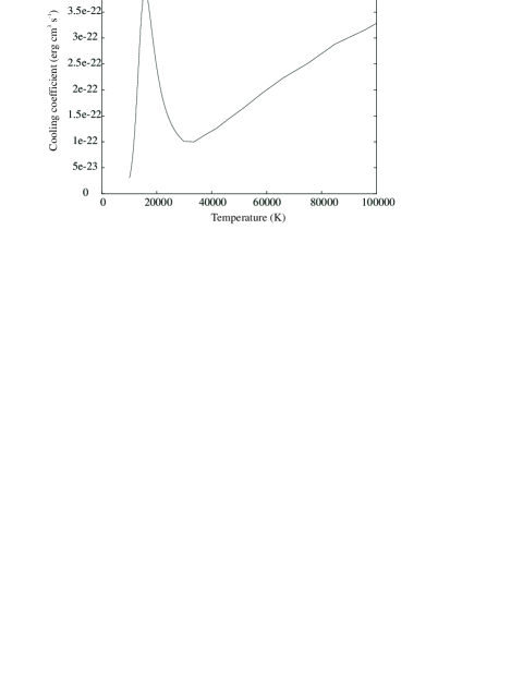
The cooling function used in this work is a combination of that used by Rossi et al. (1997) and that contained in Sutherland & Dopita (1993). At low temperatures () it is probable that the former is more accurate. However at higher temperatures this cooling function fails as it only calculates cooling due to at most singly ionised atomic species. The latter cooling function is calculated for a gas of cosmic abundances cooling from about K and it does not take account of non-equilibrium ionisation (unlike the Rossi et al. (1997) cooling function). The resulting function is plotted in Fig. 1. Tests of our implementation of the cooling have shown that it performs very well, predicting reasonably accurately the stability limit as well as the amplitude of oscillation of an overstable radiative shock wave (see Downes 1996). Note that this test is for rather strong shocks ( km s-1) and so only tests the Sutherland & Dopita (1993) cooling function.
Rossi et al. (1997) also used a constant volume heating function which cancels the cooling function at the equilibrium temperature, . Here we compare the results of simulations which use this heating term with those which simply assume that, below (K in this work) the cooling is insignificant and therefore can be set to zero. Rather than simply cutting off the cooling at we attenuate the cooling function shown in Fig. 1 as follows:
| (20) |
This effectively implies that the cooling is zero at K. Note that this means that the cooling function is a very shallow function of temperature around . The assumption of insignificant cooling below is often used in simulations of purely atomic YSO jets as, below K, the atomic cooling rate falls off rapidly (Blondin et al. 1990). We find that these two approaches to maintaining equilibrium in the initial configuration produce significantly different results. In addition we have run simulations where the heating term is proportional to the density, as might be the case if radiative transfer was occurring.
3 Initial and boundary conditions
There are two approaches to analysing the KH instability. One is to perturb a flow at a particular point in space and observe how the disturbance grows as it propagates downstream. The other is to perturb a flow everywhere and observe how the disturbance grows with time. The former is referred to as a spatial approach and has been adopted by, for example, Hardee & Norman (1988) and Hardee & Stone (1997). The latter is called the temporal approach and has been used by Bodo et al. (1994) and Rossi et al. (1997). Here we use the temporal approach.
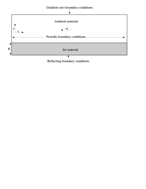
In order to do this the initial conditions were set up as shown in Fig. 2. The slab jet occupies all of the grid within 1 jet radius of the ‘lower’ edge. The boundary conditions at either end of the grid are set to periodic so that, effectively, we have a jet with infinite length. The boundary away from the jet axis is set to have gradient zero boundary conditions, while the jet axis boundary conditions are set to reflecting.
The grid cells are uniform in the direction parallel to the jet axis with a size of cm. Perpendicular to this direction the cell spacing obeys
| (21) |
where is the cell index perpendicular to the jet axis and cm. The grid size was set to 400200 cells, or about 48 jet radii. We ‘stretch’ the cells perpendicular to the jet axis in order to avoid reflections from the upper boundary. The jet radius was set at 50 cells (i.e. cm) which is typical of YSO jets (e.g. Raga 1991).
The jet to ambient density ratio was set to 1 and the jet and ambient medium were set to be in pressure equilibrium also. Three different density regimes were used: 20 cm-3, 100 cm-3 and 300 cm-3. These densities, although perhaps rather low for YSO jets (e.g. Bacciotti et al. 1995), were selected to ensure that the cooling lengths behind shocks were resolved. The pressure was chosen so that the initial temperature on the grid was K. This temperature being set as the equilibrium temperature of the system (see Sect. 2.3).
The calculation was performed in the rest frame of the jet in order to reduce the effect of advection errors on the growth of the instability. The ambient medium was given an initial velocity of Mach 10 (112 km s-1). The jet material was given a small transverse velocity perturbation:
| (22) |
where is the number of perturbation wavelengths, is the jet sound speed, is the jet radius, and are approximately 0.21, 0.42, 0.52, 0.84, 1.05, 1.68, and 2.09. These values were chosen so that the grid length corresponded to an integral number of wavelengths of each perturbation. The sine term outside the summation gives the perturbation a profile across the jet radius such that it is zero both on the axis and at the edge of the jet. Therefore, the perturbation has a velocity structure similar to that which would be produced by the first reflecting mode at all these values of . However, it is not true to say that this perturbation excites only the first reflecting mode since we do not introduce corresponding perturbations in the pressure and density.
It is well known (e.g. Bodo et al. 1994) that introducing a shear layer dampens the growth rates of all surface modes and body modes which have wavelengths shorter than the width of the layer. In simulations of adiabatic jets with high Mach numbers this is generally unimportant as the growth rates of the surface waves are usually much less than the growth rates of the body modes. However, in radiatively cooled jets analytic studies suggest that a surface mode exists which has growth rates higher than all other modes for a large range of wavelengths if the cooling function around is shallow enough (see Hardee & Stone 1997). Therefore it is important that we run simulations with different thicknesses for the shear layer in order to study the effect of this surface mode if it is present.
The jet itself is given a ‘top-hat’ velocity profile modified by a term so that a shear layer exists initially between the jet and ambient medium. Two forms of this term have been tested. The first is identical to that of Rossi et al. (1997), i.e.
| (23) |
which gives a shear layer of approximately 20 cells. The second was chosen to be
| (24) |
This gives a shear layer of about 5 cells. This latter shear layer is wide enough to be well resolved by the code, and hence avoids numerical errors which lead to spurious waves being emitted from the jet boundary. The latter was chosen for the majority of simulations in the parameter space study.
4 Analysis
The analysis of the results of these simulations to find the growth rates of the KH modes is not trivial. First the velocity perpendicular to the jet axis was averaged over 1 jet radius at a particular time. A Fourier transform of the resulting data was performed and the power contained in the wavelengths of the initial perturbation were recorded. This was done at several times during the simulation and these powers were used to derive growth rates.
The averaging process described above was carried out to reduce the effect of the different distributions of amplitude of the KH modes across the jet radius. The signal at a particular wavelength from a single row of cells parallel to the jet axis will change with distance from the axis. This signal will be given by a complicated weighted mean of the modes present. The weighting associated with a particular mode is determined by the distribution of the disturbance due to that mode across the jet. Thus, for example, if we take a row of cells located very close to the edge of the jet, the signal we receive might come primarily from surface modes. If we locate the row of cells a distance of from the jet axis the signal we will receive will be biased towards the first body mode, although it may be modified significantly by the presence of other odd index body modes. Averaging reduces the effects of these problems.
It is important to note that the averaging process described above has the effect of removing the signal from even-index body modes and it also reduces the signal from surface modes. The growth rates calculated on the basis of this averaging will be a weighted mean of the odd-index modes present at the wavelength in question, with the lower index modes being more heavily weighted.
Several tests were performed using this averaging technique for the growth of the KH instability in an adiabatic jet with a Mach number of 10 and density ratio of 1. The derived growth rates were within 20% of those predicted by linear analysis where only one mode was present. If more than one mode was present, the derived growth rates at a particular wavelength lay between the growth rates predicted from theory for the modes present at that wavelength, as expected.
5 Results
We have run 9 simulations with identical initial conditions, but with different techniques for calculating the energy loss function . None of the simulations shown here have linear growth rates which are significantly different to the adiabatic growth rates. This is in agreement with the linear results of Rossi et al. (1997), and would be expected anyway since the cooling times near equilibrium are much longer than any other time scales in the system. In addition we have run simulations, both cooled and adiabatic, to test the effect of varying the shear layers as described above. It was found, in general, that widening the shear layer, while changing the behaviour of the system for a short time at the beginning of the non-linear phase, did not significantly alter the long-term evolution of the jet.
We will begin by describing the evolution of a typical radiatively cooled simulation and comparing this with the evolution of an adiabatic simulation with identical initial conditions. We will then discuss the results of the parameter space study in terms of
-
•
the transfer of momentum from jet material to ambient material
-
•
the distribution of momentum throughout the grid
-
•
the strength of shocks produced on the jet axis
Each of these sections will be broken down into an analysis of the effect of the shear layer and an analysis of the effect of the different heating terms. All times are quoted in units of the sound crossing time . In the simulations presented here yrs.
5.1 General properties of the cooled KH instability
As already noted, the linear behaviour of the KH instability was not significantly altered by the introduction of cooling for the parameters chosen here. This would be expected since the cooling time around equilibrium is longer than any other time-scales in these simulations.
Once we enter the non-linear regime, however, cooling has a dramatic effect on the evolution of the system. This is illustrated in Fig. 3 which contains grey-scale plots of the distribution of the jet tracer variable at various times throughout an adiabatic and a cooled simulation. We can see that very little mixing occurs in the adiabatic simulation and the jet expands due to the conversion of bulk kinetic energy to internal energy by the growth of waves due to the KH instability. Differences between the adiabatic and cooled jets become noticeable at and by there are very significant differences in the distribution of jet material. The cooled jet material remains closer to the axis and, in addition, ambient material has been funneled onto the axis by the distortion on the surface of the jet. From this figure we would intuitively expect stronger shocks to form in the cooled jet as a result of this funneling of ambient material towards the axis. In fact this is not the case, due to the oblique nature of the shocks formed and also the damping of the body modes by cooling observed by Rossi et al. (1997) and predicted by Hardee & Stone (1997). We can clearly see the nature of the shocks formed in Fig. 4 which contains plots of the density for the same simulations at the same times as those shown in Fig. 3.
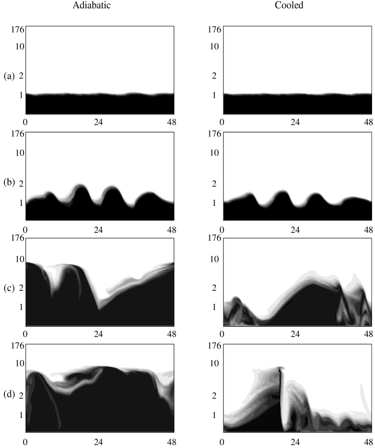
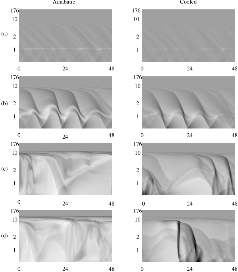
Figure 5 shows the above results in a quantitative fashion. It contains plots of the proportion of material, , lying between and which is jet material. We can see that in the adiabatic case, although a lot of jet material has moved away from the axis, almost all the material remaining near the axis originated in the jet. In contrast, if the jet is allowed to cool radiatively, we can see that only 70% of the material lying between and is jet material by the end of the simulation ().
5.2 Transfer of momentum from jet to ambient material
In this section we look at momentum transfer from material which was initially in the jet to material which was initially in the ambient medium. Note that this does not tell us about the spatial distribution of the momentum. The momentum remaining in jet material at time is defined here as
| (25) |
In the plots shown in Figs. 6 and 7 this value is normalised by .
Two adiabatic simulations were run each with an initial shear layer with a different width and it was found that, as expected, the results were not significantly different. In particular, the momentum transferred to the ambient medium differed by less than 6% throughout the entire duration of the simulation. Varying the width of the shear layer has a larger effect on the radiative jets at , as we can see in Fig. 6. The jet with the wide shear layer is initially more stable than that with the narrow shear layer. However, as noted above, the state of the two jets seems to be rather similar by .
Now we discuss the results of simulations with the ‘narrow’ shear layer (described in Sect. 2.3) with different techniques of maintaining initial cooling equilibrium. The cooling function itself is the same for all the simulations. We have run 9 more simulations corresponding to 3 different heating terms and 3 different densities, each with a jet to ambient density ratio of 1.
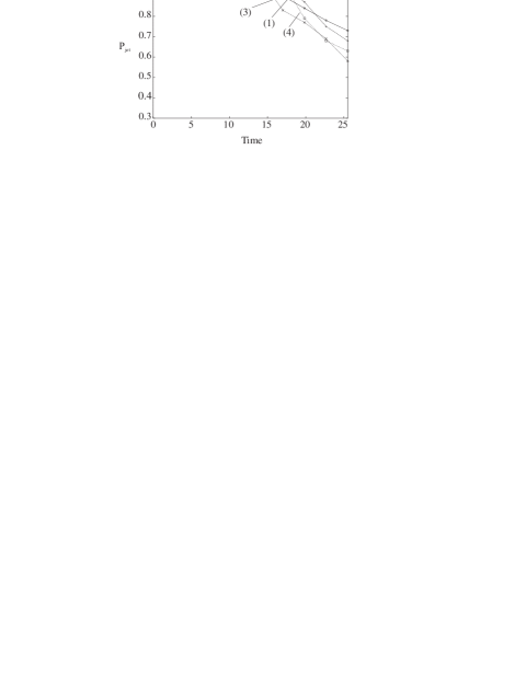
Figure 7 contains plots of the fraction of momentum remaining in jet material against time for each of the 3 different densities and each of the 3 techniques of maintaining equilibrium. Each plot also shows the behaviour of an adiabatic jet for comparison. It is clear that in all cases the radiative jets transfer momentum to the ambient material more efficiently than the adiabatic jets. It can also be seen that, for all densities, assuming insignificant cooling below causes the most efficient transfer of momentum. If a heating term proportional to the density is introduced the rate of transfer of momentum is reduced slightly. If the heating term is a constant (i.e. constant volume) then the momentum transfer is reduced more, though it still remains more efficient than in the adiabatic case.
5.3 Distribution of momentum
Here we analyse how the momentum initially contained in the jet is distributed throughout the grid with time. We define
| (26) |
where is the momentum at the grid point at time and is the length of the grid in the along the axis of the jet in grid cells and is chosen so that . In the plots shown below we normalise these values by , i.e. the momentum contained within 1 jet radius of the axis at .
We find that in both the adiabatic and the cooled cases, widening the shear layer causes a noticeable difference in results from around to with the jet with the narrow shear layer distributing its momentum throughout the grid more quickly. After this time the differences in the initial widths of the shear layers has almost no effect.
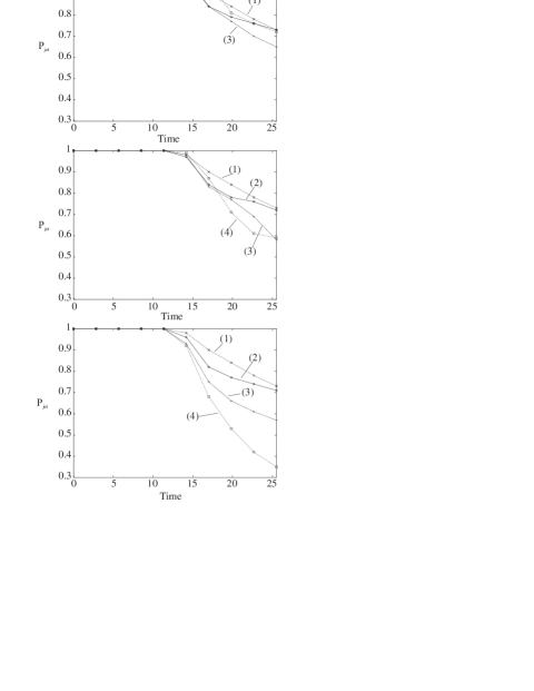
In Sect. 5.2 we noted that radiative cooling caused a more efficient transfer of momentum from jet to ambient material. However, it is clear from Fig. 9 that this momentum remains closer to the jet axis if the jet is cooled.
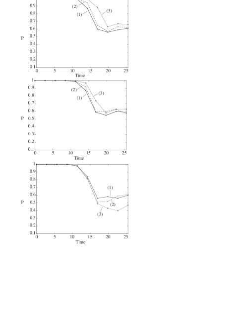
A particularly interesting result is that when the jet has entered the non-linear regime the momentum distribution enters a quasi-steady state with between 50% and 70% of the initial jet momentum remaining within 1 jet radius of the axis. This implies that the shocks formed during the growth of the instability tend not to force longitudinal momentum ‘sideways’ to beyond a couple of jet radii. It is also clear that increasing the density reduces the rate of loss of momentum from this region for the simulations with a heating term while the reverse is true for the simulations assuming that cooling is zero below .
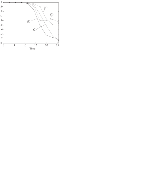
From Fig. 9 we can see that the momentum distribution attains this quasi-steady state at crossing times for all the heating terms and densities investigated here. Generally, the simulations with a constant volume heating term retain a higher proportion of jet momentum in this region. The simulations which used the assumption of insignificant cooling below lose most momentum from this region.
It is interesting to note that, for , the simulation with the assumption of insignificant cooling below is very similar to an adiabatic system in terms of the momentum distribution. However, the adiabatic system continues to transport momentum beyond after the cooled simulations have reached a quasi-steady state.
5.4 Shock strengths and morphologies
We have measured the maximum shock strength on the axis of the jet against time. Since shocks are typically smeared over 3 to 4 cells in this code we measure the maximum shock strength using the equation
| (27) |
Thus we only look at the amplitude of the velocity discontinuity in the direction parallel to the jet axis.
Figure 10 shows plots of the maximum shock strength against time for the adiabatic and cooled simulations with the wide and narrow shear layers. We can see that shocks form earlier in the adiabatic jet with the narrow shear layer and reach a maximum strength of about 50 km s-1. The jet with a wide shear layer takes slightly longer to develop shocks but, when they do form, they reach a higher amplitude of almost 70 km s-1.
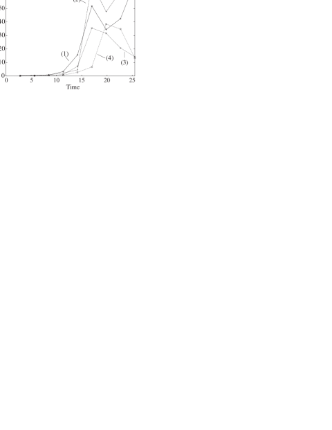
The same type of effect of the shear layer is seen in the cooled case. Here, though, the differences in the time taken for shocks to form is greater while the difference in the maximum shock strength attained throughout the simulations is less.
Figure 11 shows plots of the maximum shock strength against time for the adiabatic simulation with the narrow shear layer and the 9 other simulations with different densities and heating terms. In all cases where the heating term is either constant or proportional to the density it is clear that increasing the density slows down the development of strong shocks and reduces the maximum strength of these shocks over the duration of the simulation. The same cannot be said, however, for the simulations where we assume that cooling is insignificant below . Here the simulation with cm-3 develops stronger shocks than either of the simulations with cm-3 or 20 cm-3.
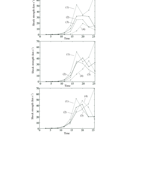
As might be expected from Sects. 5.2 and 5.3, the heating term which leads to the slowest and weakest shock development is the constant volume one. If the heating term is set proportional to the shocks are formed slightly faster and evolve to a greater strength. The simulation which simply assumes the cooling to be insignificant below forms the strongest shocks.
In general, the shocks produced by the instability in radiative jets are quite flat, but with a slight bow shape pointing towards the jet source. In the adiabatic simulations these shocks tend to be more curved with the apex of the curve pointing away from the jet source.
5.5 Proper motions
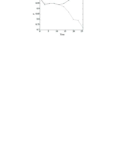
The proper motions of the shocks produced in the simulations have been measured as the motion of the shock with respect to the ambient medium. The adiabatic simulations produced shocks with proper motions in the range 0.7–0.9 while the shocks in the cooled simulations moved with proper motions of 0.3–0.9. No significant differences were found between the proper motions of shocks produced by different heating terms or densities. Strong shocks were found to move slower with respect to the jet source than weaker shocks, as would be expected from momentum balance arguments.
While making these measurements it was noted that, in cooled jets, the shock pattern tends to coalesce into 1 shock within a few crossing times of the first shocks appearing. The rate of coalescence was found to increase with the density of the jet. Shocks were not found to coalesce in the adiabatic simulations.
6 Discussion
We have performed a total of 12 different simulations of the KH instability in jets. The parameters were chosen to approximate the physical conditions thought to prevail in jets from young stellar objects.
6.1 General differences introduced by cooling
We have found that introducing cooling
-
•
increases the level of mixing between jet and ambient material
-
•
increases the amount of momentum transferred from jet material to ambient material
-
•
increases the time taken for shocks to develop in the flow
-
•
reduces the strength of these shocks
-
•
reduces the rate of decollimation of the momentum flux
The first and second of these results are somewhat surprising as they contradict the results presented by Rossi et al. (1997). However, we found it possible to reproduce the results of Rossi et al. (1997) by performing the simulations in cylindrical symmetry. Therefore we can conclude that, although in the linear regime we do not expect significant differences between the 2 symmetries, the non-linear growth of the instability is significantly affected by the choice of symmetry.
We will now explain how radiative jets can transfer more momentum to the ambient medium while the momentum flux in these systems remains better collimated than in an adiabatic system. As the KH instability grows, longitudinal momentum will be converted to internal energy by the resulting compressions and shocks within the jet. If the jet is not cooled it will, as a result, become overpressured and begin to expand and so momentum will be moved away from the jet axis. This mechanism allows longitudinal momentum to be transported away from the jet axis while still remaining in jet material. If, on the other hand, the jet is cooled this internal energy is radiated away causing the jet to remain in approximate pressure equilibrium with the surrounding medium and thus momentum will not be transported away from the jet axis in this way. In fact, as the instability grows in the cooled jet the surface of the jet develops a saw-tooth profile which steepens and eventually funnels ambient material towards the jet axis, causing mixing. It is in this way that momentum is transferred from jet to ambient material in the radiatively cooled simulations. It is interesting that the shocks produced by this process do not appear to decollimate the jet.
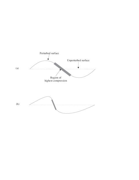
The process by which the steepening of the disturbance on the surface of the jet occurs can be understood as follows. As the jet’s surface becomes perturbed by the transverse velocity perturbation, the expanding parts of the jet begin to compress the surrounding ambient medium. This process heats both ambient and jet material near the boundary between the two. The region is then cooled and a dense filament will form at the boundary. The inertia of this filament will cause the smooth wave pattern to be converted to a saw-tooth one as the wave grows in amplitude. This process is illustrated in Fig. 12. Put another way, the waves steepen and ‘break’ earlier in the radiative than the adiabatic case because of a stronger dependence of the wave speed on its amplitude.
The shocks produced in the adiabatic jet are formed by the growth of body modes. Our results suggest that cooling of the type expected in YSO jets inhibits the development of shocks and this is in agreement with the results of Rossi et al. (1997). This is because the development of the instability takes longer due to the increased levels of cooling in low density regions and vice versa for high density regions with respect to equilibrium values (see Hardee & Stone 1997). Therefore, in a cooled jet, the time taken for shocks to develop in the jet is increased. Note however, that while this explanation is valid for these simulations, it does not imply that, in general, shocks resulting from the KH instability are weaker if cooling is introduced. We emphasize that whether this is the case in general depends on the form of the heating and cooling functions.
6.2 Effect of shear layers
Our simulations suggest that widening the shear layer does not significantly affect the long term evolution of the system.
This result is easily explained. Previous studies of the KH instability in adiabatic jets (e.g. Payne & Cohn 1985; Hardee & Norman 1988) have shown that the surface modes do not grow as fast as the body modes in high Mach number flows for . A wide shear layer tends to damp the growth of surface modes and body modes with wavelengths less than the width of the layer (for example, Bodo et al. 1994). Therefore, although widening the shear layer will damp surface modes, we know that in an adiabatic jet these modes do not have a significant effect on the jet anyway. Since it is these modes which are expected to disrupt the jet and thus cause mixing and transfer of momentum from jet material to ambient material, we do not expect widening the shear layer to have much effect on momentum transfer in the adiabatic case. According to Hardee & Stone (1997) introduction of cooling can allow a new surface mode to grow which has higher growth rates than any other modes present if the cooling function is shallow enough around . In our simulations it is difficult to tell whether the cooling function is shallow enough around as it is a non-equilibrium one and we also include energy dumped into ionisation in our calculations. Since the differences in growth rates introduced by the narrowing of the shear layer are of order a few percent, it seems reasonable to say that this surface mode does not exist, or at least has a very low growth rate, for the energy loss functions studied here.
6.3 Effect of changing the heating function
Detectable differences were found between simulations which included a constant volume heating term and those which included a heating term proportional to . Generally, the inclusion of the former resulted in behaviour more similar to an adiabatic system than simulations with the latter kind of heating term, though this difference is relatively small.
Simulations with the assumption that the cooling is insignificant below were dramatically different from adiabatic simulations and were generally more unstable than the simulations which used a heating function to maintain initial equilibrium. This difference is unlikely to arise from the growth of the surface mode mentioned by Hardee & Stone (1997) because of the very low level of the cooling around for the modified cooling function described in Eq. 20. It is more likely to be due to the fact that there is no heating term in the system and this allows the instability to grow faster than in the other cooled systems.
The injection of energy by a heating term makes the system as a whole more similar to an adiabatic one. It is plausible to suggest that the lack of a heating term will therefore accentuate any differences between adiabatic and cooled systems.
6.4 Differences between slab and cylindrical symmetry
As already stated, the results of simulations of the cooled KH instability in slab and cylindrical symmetry differ in 2 respects. In slab symmetry the introduction of cooling
-
•
increases the level of mixing between jet and ambient material
-
•
increases the amount of momentum transferred from jet material to ambient material
whereas the introduction of cooling in cylindrical symmetry does the opposite.
We can understand this as follows. The increase in mixing and momentum transfer in slab symmetry results from disturbances on the surface of the jet steepening due to cooling as discussed in Sect. 6.1. While we do not expect this steepening process to be significantly modified by the choice of symmetry we note that axisymmetric waves of a given amplitude on the surface of the jet require higher pressures (and hence higher temperatures) on the jet axis in cylindrical symmetry. This is because the amplitude of an axisymmetric wave in cylindrical symmetry goes as whereas it is independent of in slab symmetry. Thus if the system is cooled, and the cooling function is an increasing function of , we expect cooling to damp the waves more in cylindrical than in slab symmetry. Hence the disturbances on the surface of the jet will be lower in amplitude and take longer to steepen. This is precisely what we observe in cylindrically symmetric simulations. By the time the waves have steepened significantly the corresponding adiabatic jet will have disrupted.
Hence we conclude that, while slab symmetric simulations are adequate to approximate the linear behaviour of the axisymmetric modes of the KH instability in cooled cylindrical jets, such simulations give misleading results in the the non-linear regime. In principle one would expect the above argument to hold for studies which examine the growth of the helical modes of the KH instability using slab symmetric simulations of the sinusoidal modes (e.g. Stone et al. 1997). However, this assumes that the most significant waves are ones which pass through the body of the jet rather than along its surface.
Acknowledgements.
This work has been partly supported by Forbairt grant number BR/93/013/. We would also like to thank Alex Raga, Stephen O’Sullivan, Milena Micono, Jim Stone, Silvano Massaglia and Phil Hardee for useful discussions during the preparation of this paper.7 References
Bacciotti, E., Chiuderi, C., Oliva, E., 1995, A&A 296, 185
Bachiller, R., 1996, ARA&A 34, 111
Birkinshaw, M., 1991, in: Beams and Jets in Astrophysics, ed. P. Hughes, (Cambridge: CUP), p. 278
Blondin, J.M., Fryxell, B.A., Königl, A., 1990, ApJ 360, 370
Bodo, G., Massaglia, S., Ferrari, A., Trussoni, E., 1994, A&A 283, 655
Bührke, T., Mundt, R., Ray, T.P., 1988, A&A 200, 99
Downes, T.P., 1996, PhD Thesis (University of Dublin, Ireland)
Edwards, S.E., Ray, T.P., Mundt, R., 1993, in: Protostars and Planets III, eds. E.H. Levy J.I. Lunine, (Tucson: University of Arizona), p. 567
Eislöffel, J., Davis, C.J., Ray, T.P., Mundt, R., 1994 ApJ 422, L91
Falle, S.A.E.G., Raga, A.C., 1995, MNRAS 272, 785
Harris, D.E., Biretta, J.A., Junor, W., 1997, MNRAS 284, L21
Hardee, P.E., Cooper, M.A., Clarke, D.A., 1994, ApJ 424, 126
Hardee, P.E., Stone, J.M., 1997, ApJ 483, 121
Hardee, P.E., Norman, M.L., 1988, ApJ 334, 70
Hartigan, P., Morse, J.A., Raymond, J., 1994, ApJ 436, 125
Lopéz, R., Raga, A., Riera, A., Anglada, G., Estalella, R., 1995, MNRAS 274, L19
Neckel, Th., Staude, H.J., 1987, ApJ 322, L27
Padman, R., Bence, S., Richer, J., 1997, in: Herbig-Haro Outflows and the Birth of Low Mass Stars, IAU Symposium No. 182, eds. B. Reipurth & C. Bertout, (Dordrecht: Kluwer Academic Publishers, p. 123
Payne, D.G., Cohn, H., 1985, ApJ 291, 655
Raga, A.C., 1991, AJ 101, 1472
Raga, A.C., Canto, J., Binette, L., Calvet, N., 1990, ApJ 364, 601
Ray, T.P., 1996, in: Proceedings of the NATO ASI on Solar and Astrophysical MHD Flows, ed. K. Tsinganos, (Dordrech: Kluwer Academic Publishers), p. 539
Ray, T.P., Mundt, R., Dyson, J., Falle, S.A.E.G., Raga, A., 1996, ApJ 468, L103
Reipurth, B., Hartigan, P., Heathcote, S., Morse, J.A., Bally, J., 1997, AJ 114, 757
Rossi, P., Bodo, G., Massaglia, S., Ferrari, A., 1997, A&A 321, 672
Stone, J.M., Norman, M.L., 1993, ApJ 413, 210
Stone, J.M., Norman, M.L., 1994, ApJ 420, 237
Stone, J.M., Xu, J., Hardee, P.E., 1997, ApJ 483, 136
Sutherland, R.S., Dopita, M.A., 1993, ApJS 88, 253
van Leer, B., 1977, J. Comp. Phys. 23, 276
von Neumann, J., Richtmyer, R.D., 1950, J. Appl. Phys. 21, 232