The use of high magnification microlensing events in discovering extra-solar planets

Abstract

Hundreds of gravitational microlensing events have now been detected towards the Galactic bulge, with many more to come. The detection of fine structure in these events has been theorized to be an excellent way to discover extra-solar planetary systems along the line-of-sight to the Galactic center. We show that by focusing on high magnification events the probability of detecting planets of Jupiter mass or greater in the lensing zone (.6 -1.6 $R_{E}$) is nearly 100%, with the probability remaining high down to Saturn masses and substantial even at 10 Earth masses. This high probability allows a nearly definitive statement to made about the existence of lensing zone planets in each such system that undergoes high magnification. One might expect lightcurve deviations caused by the source passing near the small primary lens caustic to be small due to the large distance of the perturbing planet, but this effect is overcome by the high magnification. High magnification events are relatively rare (e.g. $\sim 1/20$th of events have peak magnifications greater than 20), but they occur regularly and the peak can be predicted in advance, allowing extra-solar planet detection with a relatively small use of resources over a relatively small amount of time.

Physics Department, University of California, San Diego, CA 92093

1 Introduction

Microlensing has become a useful tool in astronomy for discovering and characterizing populations of objects too faint to be seen by conventional methods. By repeatedly monitoring millions of stars several groups have now detected the rare brightenings that occur when a dark object passes between the Earth and a distant source star Alcock et al. (1993); Aubourg et al. (1993); Udalski et al. (1993); Alard et al. ​ (1995). These detections have now become routine with hundreds of events reported towards the Galactic bulge, mostly by the MACHO collaboration Alcock, et al. (1997a); Alcock et al. (1996). The reliable detection of large numbers of such lensing events allows one to use them for several auxiliary purposes. For example, relatively rare microlensing “fine structure” events, where deviations from the simple brightening formula Paczynski (1986); Griest (1991) are apparent, can be searched for. These have allowed several new effects to be observed, such as parallax motion Gould (1992, 1994); Alcock et al. (1995), the finite size and proper motion of the source star Alcock et al. (1997b), and binary lensing Mao & Paczynski (1991); Udalski et al. (1994); Pratt et al. (1995).

Here we consider the special case of binary lensing when one (or more) of the companions is actually a planet orbiting the primary lens. This possibility has been investigated by several groups starting with ?) and ?). They found the remarkable result that detectable fine structure occurs relatively frequently even for rather low mass planets. For example, ?) find for a Jupiter mass planet 5 AU from a solar mass star the probability of detecting the fine structure caused by the jupiter is about 17%, while for a Saturn-like planet the probability is about 3%. These relatively high probabilities occur when the planet is in the “lensing zone” to be discussed later, but they imply that many planetary systems could be discovered if a systematic search for microlensing fine structure were made. The lightcurve deviations caused by a planet last only a few hours or days (depending upon the mass of the planet) and can occur at any time during the much longer ($\sim 40$ days) primary lensing event. In order to not miss these short excursions, round-the-clock monitoring would be required, implying dedicated telescopes at several locations. In return, dozens to hundreds of planetary detections could be made, more than by other proposed detection methods. Thus microlensing may be the best way to gather statistics on the frequency, mass distribution, and semi-major axis distribution of planets. Microlensing is also sensitive to planetary systems throughout the Galaxy and not just in the solar neighborhood as are most other planet search techniques. The main disadvantage to microlensing is that further study of individual systems is probably impossible.

Following the early work, contributions have been made by several other groups. ?) calculated detection probabilities, ?) and ?) extended to Earth mass planets by including the finite source effect, ?) discussed extraction of physical parameters from observational data, ?), ?), and ?) calculated the number of expected detections for realistic observing strategies.

2 Microlensing formulas, caustics, and magnification maps

Microlensing occurs when an intervening stellar mass lens passes close to the line-of-sight between an observer and a distant source star. For Galactic distances, if the lens is a single point-mass, two images form with a separation of milli-arcseconds, too small to resolve. However, since the sum of the areas of the images is larger than the projected area of the source, the magnification, which is given by the ratio of these areas, can be significant. When the source lies directly behind the lens, the image becomes a ring of radius $R_{E}$, and the magnification theoretically becomes infinite. Points in the source plane where the magnification is infinite are called caustics, and the positions of the images of these caustics are called critical curves. For a single lens, the caustic is single point behind the lens, and the critical curve is the Einstein ring.

The scale of the microlensing effect is set by the Einstein ring

$$R_{E}=\left(4Gm_{l}Lx^{\prime}(1-x^{\prime})\over c^{2}\right)^{1/2}=612\rm{R_{\odot}}\left({m_{l}\over\rm{M_{\odot}}}{L\over{\rm kpc}}x^{\prime}(1-x^{\prime})\right)^{1/2},$$ (1)

where $m_{l}$ is the mass of the primary lens, $L=D_{os}$ is the distance to the source star, $x^{\prime}=D_{ol}/D_{os}$ is the fractional distance of the lens, $\rm{R_{\odot}}$ is the solar radius, and $\rm{M_{\odot}}$ is the solar mass. Throughout, we will scale all lengths to $R_{E}$. For convenience note 1 AU is $214.94\rm{R_{\odot}}$.

When the lens consists of two point-like objects, the caustic positions and shapes depend upon the planet to lens mass ratio $q=m_{p}/m_{l}$, and the projected planet-lens separation, $x_{p}$. The primary lens is assumed to reside at the origin, and the planet is along the positive x-axis at $x_{p}$ in units of $R_{E}$. For arbitrary distances and mass ratios the caustic structure can be complicated, but for small values of $q$, and for $x_{p}$ not precisely unity, the picture is simple. The point-like single lens caustic becomes a tiny wedge-like caustic, still located near $x=0$, while one or two new caustics appear depending on the planet position. For planets far from the lens ($x_{p}>1$), there is one new caustic, a small diamond-shaped planetary caustic located on the same side of the lens as the planet, while for $x_{p}<1$, two small heart-shaped caustics appear close together on the opposite side of the lens. As discussed in the appendix, the position of these caustics is given approximately by $x_{c}=(x_{p}^{2}-1)/x_{p}$. Figure 1 shows the caustics for the case of $q=0.003$, corresponding to a Jupiter mass planet around a $0.3\rm{M_{\odot}}$ star. Panel (a) is for $x_{p}=1.3$ and panel (b) is for $x_{p}=1/x_{p}=0.769$. We will call the caustic near $x=0$ the “central” or “primary lens” caustic, and the other caustics the “planetary” caustics.

The relative motion of the source, lens-system, and observer can be described as the source moving behind a static lens plane described by the projected positions of the lens, planet, and caustics. We work in the lens plane throughout and project physical sizes such as the source stellar radius into dimensionless numbers in the lens plane by multiplying by $x^{\prime}$ and dividing by $R_{E}$. If the planet orbits the primary lens in a plane other than the lens plane, its position is also projected into the lens plane.

For single-point lenses high magnification events occur when the source comes near the caustic at $x=0$. If $u$ is the projected distance of the source from the lens (in units of $R_{E}$ in the lens plane), the magnification is $A=(u^{2}+2)u^{-1}(u^{2}+4)^{-1/2}\sim u^{-1}$ for $A$ large. The peak magnification $A_{max}$ occurs at $u_{\rm min}$, the distance of closest approach. The trajectory intersects a circle of radius $u_{\rm min}$ at its closest approach, with $\beta$ being the angle between this intersection point and the positive x-axis. With the addition of a planet we continue to define high magnification events as those caused by the source approaching the central caustic. For planetary mass binary systems, the lightcurve will be very close to that of a single lens for most of its duration.

Planetary fine-structure in the high magnification case will arise due to the difference between a point caustic and the wedge-like central caustic. If $A\sim 1/u$ as the source approaches the caustic then the size of the deviation $\delta=dA/A\sim-Adu$, where $du$ is the shift in the caustic position due to the planet. It is shown in the appendix that the size of the central caustic along the x-axis is

$$u_{c}={qx_{p}\over(x_{p}-1)^{2}},$$ (2)

and that this formula is invariant under a “duality” transformation $x_{p}\rightarrow 1/x_{p}$. As described in the appendix this formula is good for $q<<1$ and $x_{p}$ not near unity. Thus for high magnification events, we expect deviations of order

$$\delta\sim u_{c}A.$$ (3)

This estimate of lightcurve deviation is in rough agreement with the more precise calculations of the next sections, and the caustic size estimate (eq. 2) is excellent, as can be seen in Figure 2. Figure 2 shows close-ups of the central caustic for various planetary positions and planetary mass ratios. The $x_{p}\rightarrow 1/x_{p}$ symmetry is also apparent in these figures.

Especially useful when discussing the detection of planets or the probability of certain types of events occurring, are magnification maps of the source plane, projected onto the lens plane. These are formed by imagining a source at each point in the plane and calculating the resulting image sizes and resulting magnifications. Observationally, one measures the microlensing lightcurve, the apparent brightness of a star as a function of time, and this is completely described by a track through this magnification map. The duration of the event depends upon the size of the Einstein ring and the relative projected transverse speed $v_{\perp}$ of the lens system. We will divide all times by $t_{E}=R_{E}/v_{\perp}$, so the time to cross the Einstein ring diameter is $\Delta t=2.0$.

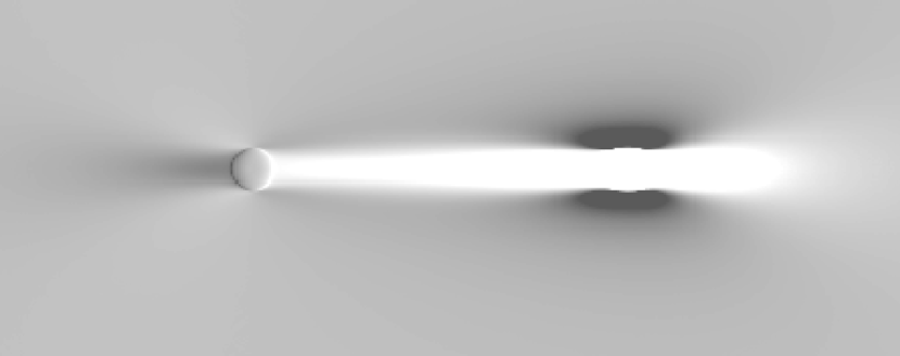
Figure 3: Example magnification maps show the ratio of planetary to single lens magnification in the source plane. Light areas show positive deviations (ratios greater than one) and dark areas show negative deviations. All panels are for $q=10^{-4}$, a 10 Earth-mass planet around a $0.3\rm{M_{\odot}}$ star. Panel (a) shows $x_{p}=1.3$ with a source radius of $u_{*}=0.003$, while panel (b) shows an example of $x_{p}<1$ ($x_{p}=0.8$) with the same source radius. Panel (c) shows $x_{p}=1.3$, but with the large source radius of $u_{*}=0.03$.

Examples of magnification maps and the resulting lightcurves can be found in ?), and ?), and several other places. Figure 3 shows some example maps and Figure 4 shows some example lightcurves.

There are several techniques to calculate such maps in practice. For point-like lenses, the lens equation in complex notation is given by (e.g. Witt 1990)

$$z_{s}=z+\sum_{j}m_{j}/({\bar{z}_{j}}-{\bar{z}}),$$ (4)

where $z_{j}=x_{j}+iy_{j}$ are the positions of the point masses in the lens plane, $z_{s}=x_{s}+iy_{s}$ is the position of the source, $z=x_{i}+iy_{i}$ are the position of the images, and the bar denotes complex conjugation. We can rescale this equation by dividing all lengths by $R_{E}$ and all masses by $m_{l}$, and specialize to just one planet to get

$$z_{s}=z-1/{\bar{z}}+q/(x_{p}-{\bar{z}}).$$ (5)

One sees that the mapping from an image position at $z$ to a source position at $z_{s}$ is one-to-one and extremely simple; however the reverse mapping requires solving the above equation for $z$, and results in a 5th degree polynomial in $z_{s}$ (see e.g. Witt 1990). The partial magnifications are given by the Jacobian of the mapping from the source to lens plane evaluated at the image positions.

$$A_{i}=\left(1-{\partial z_{s}\over\partial{\bar{z}}}{\bar{\partial z_{s}\over\partial{\bar{z}}}}\right)^{-1},$$ (6)

where the sign of $A$ gives the parity of the image, and in our case ${\partial z_{s}/\partial{\bar{z}}}=1/z^{2}+q/(z-x_{p})^{2}$. Caustics and critical curves are found as points where $A_{i}=\infty$. The total magnification is just the sum of the absolute values, $A=\sum_{i}|A_{i}|$.

The most direct way to create a magnification map is to solve for $A$ at each point in the source plane by solving the 5th degree polynomial. When the source is inside a caustic there are 5 images, while if the source is outside the caustics there are two spurious solutions and only 3 images. In the later case, one of these images is behind the lens and is very small and the other two are important. A complication of this approach occurs when the mass of the planet is small. The magnification map varies on scales smaller than the planetary Einstein ring $R_{p}$, which can be small compared to the size of the projected source star radius. Thus one must integrate the magnification over the limb-darkened source profile to get an accurate total magnification. The caustic structure gives rise to singularities in $A$, which make this integration tricky. (See ?), ?), ?), for examples of this approach). We have developed computer programs that successfully implement this approach, but they are rather slow.

Alternatively, one can note the simplicity of the mapping from image to source plane, and simply cover the image plane densely with “photons” and then map them back to their source positions. The resulting density of source photons is proportional to the ratio of image to source areas, and therefore proportional to the magnification. See ?) for an example of this method. This method intrinsically incorporates the finite source effect, since one must bin the source photons. The bin size is the effective source size. To consider a larger source size, or to include a round source with limb-darkening, one merely convolves the magnification map with a kernel made from the desired source profile. We mainly used this method in creating our maps, though we checked them in various ways using direct solution.

Lightcurves of single lens microlensing are simple smooth curves Paczynski (1986); Griest (1991), while if a planet exists there can in addition be several sharp peaks. The durations of these peaks typically scale with $R_{p}\propto\sqrt{q}$, and last only a day or two, or even only a few hours, a time to be compared with the typical primary lens event duration of 40 days Alcock, et al. (1997a). An nice set of examples of both magnification maps and lightcurves can be found in ?). For both maps and lightcurves we plot residuals

$$\delta={\Delta A\over A}={A_{binary}-A_{single}\over A_{single}}.$$ (7)

In Figure 3 we show some maps for $q=10^{-4}$. Figure 3(a) shows $x_{p}=1.3$ where there is only one planetary caustic, and Figure 3(b) shows $x_{p}=0.8$ where there are two planetary caustics on the other side of the central caustic. The lightcurves in Figure 4 are for $q=0.003$, $x_{p}=1.5$, $u_{\rm min}=0.05$, and various angles of approach. Note the relatively simple structure of these high magnification lightcurves (with exception of the trajectory along the x-axis which also hits the planetary caustic).

The method of magnification maps lets us investigate the effects of sources of different radii. Once a high resolution map is produced it can be quickly convolved with any of various source sizes and profiles, and the lightcurves and probabilities recomputed. For our convolution kernel we use a limb-darkened profile given by $I(r)=.4+.6\sqrt{1+r^{2}/R_{*}^{2}}$, where $R_{*}$ is the stellar radius, $r$ is the distance from the center of the star, and $I$ is normalized to give a total flux equal to the preconvolution flux. The maps in Figure 3(a) and 3(b) were convolved with a kernel of radius $u_{*}=0.003$, while Figure 3(c) is for a source radius of $u_{*}=0.03$. Note these radii are in units of the Einstein ring (eq. 1) and projected into the lens plane. So for example, a typical main sequence bulge star of radius $R_{*}=3\rm{R_{\odot}}$ projects to $u_{*}=0.003$ if the lens is at 4 kpc, and to $u_{*}=0.0084$ if the lens is at 7 kpc. The source is assumed to be at 8 kpc and the primary lens to have $m_{l}=0.3\rm{M_{\odot}}$ in these examples. A giant star of radius $10\rm{R_{\odot}}$ projects to $u_{*}=0.01$ for $x^{\prime}=0.5$, and $u_{*}=0.028$ for $x^{\prime}=0.875$. The map of Figure 3(c) is therefore descriptive of $30\rm{R_{\odot}}$ star with a lens system at 4 kpc or a $10\rm{R_{\odot}}$ source with a lens system at 7 kpc. An interesting feature of Figure 3(c) is the circular ring around the central caustic. There is a jump in magnification as the limb of the source star crosses the caustic. However, as the star covers more of the region around the caustic, a cancellation occurs since there is a negative deviation on one side of the caustic and a positive deviation on the other.

In Figure 5 we show the result of increasing source size on the deviation lightcurves. The lightcurves are all for $q=10^{-4}$, $x_{p}=1.3$, $u_{\rm min}=0.02$, and $\beta=50^{0}$. As expected Gould (1994); Nemiroff & Wickramasinghe (1991); Witt & Mao (1994); Alcock et al. (1997b), as the source radius increases the amplitude of the signal decreases and the duration of the deviation increases. When the star radius is increased to $u_{*}=0.03$, then it actually crosses the central caustic giving rise to two bumps on the lightcurve. These bumps occur when the trajectory crosses the ring seen in Figure 3(c). If detected, these bumps are very useful since the star is in effect resolved, and the time between the bumps allows the projected transverse velocity to be measured. For high magnification events the width (and height) of these bumps are determined by the size of the central caustic and so information about $q$ and $x_{p}$ can also be gleaned. In Figures 3 and 5, however, the width of the ring and the bumps are not determined by the size of the central caustic, but by the resolution of our underlying magnification map. Extraction of planetary parameters from high magnification events will be discussed in more detail elsewhere Griest & Safizadeh (1998).

3 Detecting Planets

Current experiments to search for planets and other microlensing fine structure piggy-back off the very successful MACHO collaboration survey alert system Alcock et al. (1996); Pratt et al. (1995). The MACHO collaboration monitors millions of stars each night and checks them for microlensing. When a candidate microlensing event is detected, an alert is sent by email to any interested party [http://darkstar.astro.washington.edu; macho@astro.washington.edu]. Two main follow-up collaborations are underway: The MACHO GMAN collaboration Alcock et al. (1996); Pratt et al. (1995), and the PLANET collaboration Albrow et al. (1997). GMAN has detected parallax events, the finite source size and proper motion fine structure, as well as several binary lens events. PLANET has followed many events and detected much fine structure as well. Two new survey systems, EROS II and OGLE II, soon plan to generate alerts, and new additions to the follow-up networks should make coverage of the short duration planetary deviations more complete.

Several groups have now calculated the probabilities that a well-monitored microlensing alert will give rise to planetary fine structure. In calculating probabilities, workers calculated typical lightcurves caused by planetary systems and then defined a detection statistic. For example, ?) and ?) defined “detectable” as at least one lightcurve point inside an area around the planetary caustic. ?) considered a planet detectable if any point on the lightcurve deviated by more than 5% from the single lens case. ?) defined detectable as the lightcurve deviating by more than 4% for a period of $t_{E}/200$. Gould & Loeb found that for a Jupiter mass planet at a distance of 5 AU from its sun, the probability of detection thus defined was nearly 17%. Given that Jupiter’s mass is $0.001\rm{M_{\odot}}$, it was remarkable that the detection probability was so high. They explained this in terms of “resonant” lensing, which occurs when the planet is near the Einstein ring radius ($x_{p}\approx 1$), and thus discovered the “lensing zone”. As discussed in detail in the appendix we define the lensing zone as the range $0.618\leq x_{p}\leq 1.618$. For a Saturn mass planet their detection probability dropped to 3%, and for smaller mass planets was even smaller.

Though they performed a very complete calculation, Gould & Loeb made various approximations. For example, they did not calculate the deviation from a magnification map, but approximated the region of 5% deviation as a long rectangular box in the source plane. They did not include finite source effects, which should not be large for the Jupiter and Saturn mass planets upon which they concentrated, but which could be large for Uranus or Earth mass planets.

By including finite source size effects ?) and ?) continued the calculation to lower mass planets where the finite size of the source star can be important. Bennett & Rhie found probabilities of about 2% for masses as low as Earth mass. ?), ?), and ?) calculated in detail the number of expected planetary detections for several realistic observing scenarios, and now several groups are undertaking extensive microlensing searches for planets. See ?), ?), or ?) for reviews. The basic plan is to monitor continuously all bulge stars undergoing microlensing with the hope of finding planetary signals in a few percent of them.

4 High magnification events

Planetary magnification maps have their most pronounced deviations from single-lens maps near the planetary caustics. The size of these caustics scale directly with the planet-lens mass ratio, and they are located roughly at positions given by eq. 9. Thus the probability of detecting a planet is roughly proportional to the angle averaged cross-sectional area of this region and this is how ?) and ?) calculated planetary detection probabilities. ?) also pointed out that the region of large deviation continues on a line from the planetary caustic towards the primary lens.

Gould & Loeb state that in order to get a large deviation the planet must come near one of the two primary lens images. This is equivalent to saying that large deviations occur when the source is near the planetary caustics. In this paper, we point out that for high magnification events, when the source comes very close to the very small central caustic, large deviations from a single lens lightcurve also occur. Thus, even though the planet is not near one of the primary lens images, planet detection can occur. This is because the high magnification makes the small changes in the central caustic detectable. In summary, very close to the lens center, the difference between the circularly symmetric single-lens caustic and the tiny wedge-like binary central caustic causes measurable asymmetries in the lightcurve. Examples of these caustics are given in Figure 2, and example lightcurves are given in Figure 4. Note from Figure 4 that the structure of high magnification lightcurves is typically simpler than the structure of planetary caustic crossing lightcurves.

In order to quantify this effect, we used our magnification maps to calculate a large number of lightcurves. For comparison purposes, we defined several “detection criteria”. $P_{5}$ is the Gould & Loeb criteria that at least one point has a deviation of more than 5% from the single lens case. $P_{4}$ is our analogue of the Bennett & Rhie criteria that the event have a time of at least $t_{E}/200$ with more than a 4% deviation. As a challenge to observers, we also defined $P_{1}$, where the planet is assumed to be detectable if it spends a duration of at least $t_{E}/200$ with a deviation from the single lens case of at least 1%. Finally, we define $P_{\chi}$ using a $\chi^{2}$ statistic. We define $\chi_{p}^{2}=\sum\delta_{i}^{2}$ where the sum is over all points for which $u<0.2$, that is, the total squared deviation for points during the time when $A\geq 20$. We define a planet as detectable if $\chi_{p}^{2}\geq 0.04$, a number set by trial and error to correspond approximately to the sensitivity of $P_{5}$ and $P_{4}$. If the photometric measurement errors were $\sigma_{i}$, this value would correspond to a chi-square of $0.04/\sigma_{i}^{2}$.

Note that in calculating the deviation, Gould & Loeb subtracted a single lens at $x_{l}=0$ with the primary lens mass unchanged, while Bennett & Rhie subtracted a single lens of mass $m_{l}+m_{p}$ at the center-of-mass position. We tried both these subtraction schemes and did not find any significant difference. We use the deviation ratio $\delta=(A_{bin}-A_{sing})/A_{sing}$, since this quantity has constant magnitude errors as the magnification increases, close to what happens in a CCD observation.

To investigate high amplification events we took a sample of events with $u_{\rm min}\leq u_{\rm th}$, for $u_{\rm th}=0.1,0.05,0.03$, and $0.02$, corresponding respectively to single-lens magnifications of at least 10, 20, 33, and 50. The quantity $u_{\rm min}$ is the distance of closest approach of the source to the primary lens (in units of $R_{E}$). The maximum magnification $A_{max}\simeq 1/u_{\rm min}$ for $A_{max}\gg 1$. Given $u_{th}$, the probability of an event occurring with $u_{min}\leq u_{th}$ is known a priori to be equal to $u_{\rm th}/u_{\rm crit}$, where it is assumed that every event with primary lens magnification greater than $A_{\rm crit}$ is alerted upon and monitored ($u_{\rm crit}=1$ for $A_{\rm crit}=1.34$). So for example with $u_{\rm crit}=1$, roughly 3% of monitored events will have $u_{min}\leq 0.03$.

Figures 6 through 9 show the results of the probability calculations. Remarkable is the very high probability for detecting planets within the lensing zone. Figure 6 ($q=0.003$) shows a Jupiter mass planet around a $0.3\rm{M_{\odot}}$ star. Figure 7 ($q=0.001$) shows a Saturn mass planet around a $0.3\rm{M_{\odot}}$ star, or equivalently a Jupiter mass planet around 1 $\rm{M_{\odot}}$ star. Figure 8 ($q=10^{-4}$) shows a 10 Earth-mass planet around a $0.3\rm{M_{\odot}}$ star.

For $u_{\rm th}=0.02$ or $0.03$, and using $P_{5}$, the least sensitive of our detection criteria, basically 100% of Jupiter mass planets would be detected over the entire lensing zone and substantially beyond it. As indicated by eq. 3, the lensing zone probabilities drop as $u_{\rm th}$ increases and therefore $A_{max}$ decreases, to as low as 90% for $u_{\rm th}=0.05$ and to as low as 80% for $u_{\rm th}=0.1$. The $\chi_{p}^{2}$ statistic $P_{\chi}$ performs similarly or slightly better than $P_{4}$ and $P_{5}$ over the entire range. If one could use $P_{1}$ by detecting 1% deviations in the lightcurve then the detection probabilities would remain near 100% far beyond the lensing zone for all values of $u_{\rm th}$.

For Saturn mass planets, Figure 7 shows that probabilities are also near 100% inside the lensing zone, with a minimum of 90% for $u_{\rm th}=0.02$, and a minimum of 80% detected for $u_{\rm th}=0.03$. The drop-off in sensitivity is quite rapid outside the lensing zone and for larger values of $u_{\rm th}$, but stays near 100% at $x_{p}\approx 1$, and above 40% even at the edge of the $u_{\rm th}=0.1$ zone. If one could detect 1% deviations, then the probability is again nearly 100% over a wide range of $x_{p}$.

We note a duality invariance $x_{p}\rightarrow 1/x_{p}$ in the probability plots for high magnification events. The probability of detecting a planet at $x_{p}=0.5$ is the same as detecting a planet at $x_{p}=2$. This is because the central caustic is almost identical under this transformation (see eq. 2 and Figure 2). The duality symmetry also shows up in the position of the planetary caustics: $x_{p}$ and $1/x_{p}$ give caustics at the same $x_{c}$ according to eq. 9 (see Figure 1). This symmetry implies a degeneracy in determining the planet position from the lightcurve for high magnification events. High magnification lightcurves with a planet at $x_{p}$ will be almost identical to those with a planet at $1/x_{p}$ in most cases. There are also potential degeneracies between planetary mass and distance, and these will be considered elsewhere Griest & Safizadeh (1998). See ?) for an extensive discussion of degeneracies for planetary caustic events.

Figures 8 and 9 show the probabilities for 10 Earth-mass planets ($q=10^{-4}\rm{M_{\odot}}$). From eq. 2, we expect the size of the deviations to drop by a factor of 10 from the $q=0.001$ case, so we expect small probabilities when using $P_{4}$ or $P_{5}$. Also we expect statistics such as $P_{4}$ which require a minimum time above a threshold to lose sensitivity in comparison with $P_{5}$ which requires only one deviant point. These expectations are born out in Figure 8 which shows a maximum probability of of $\sim 80$% near $x_{p}\approx 1$, dropping rapidly even inside the lensing zone, and probabilities below 1% at the edge of the lensing zone. $P_{1}$ fares much better, giving probabilities 80% – 100% near the zone center, dropping to 20% – 50% near the zone edge.

In order to test the effect of the finite source size on our probabilities we convolved each map with a kernel representing a limb-darkened source star of various radii, and then recalculated the probabilities. For $q=0.003$ we found no significant differences with radii up to $u_{*}=0.01$ corresponding to a typical giant star at a distance halfway to the Galactic Center. For $q=10^{-4}$, however, the effect is quite apparent, as is shown in Figures 8 and 9. For $u_{*}=0.01$, the peak $P_{5}$ or $P_{4}$ probabilities are less than 35% with a rapid drop even inside the lensing zone. In this case, the convolution has caused the maximum deviations due to the central caustic to drop below 4%, so that the detections are not actually “high magnification” events but rather are caused by trajectories which pass through the planetary caustic region. This explains the counter-intuitive result that the $u_{\rm th}=0.1$ case has a higher probability than the $u_{\rm th}=0.02$ case. Low values of $u_{\rm th}$ force the trajectories to pass near the origin, while higher values include trajectories that are more likely to hit the planetary caustic. If 1% deviations could be detected the $P_{1}$ statistic gives high probabilities even for 10 Earth-mass planets and giant source stars. The higher probabilities of Figure 8 show that the central caustic is still important for $u_{*}=0.003$.

We note that all the probabilities calculated here are for the projected lens-planet separation. To find the probability of detecting a planetary system with a given semi-major axis our probabilities must be averaged over the possible inclination angles of the planetary system. To find the probability of finding a planet of a given mass one must then average over a distribution of semi-major axes, and also over the density of planetary systems along the line-of-sight, taking into account the variation of $x^{\prime}$. See ?) for an example. This calculation will be presented elsewhere Griest & Safizadeh (1998), but see Section 6 for a caveat.

5 Discussion

High magnification events have both advantages and disadvantages when compared with ordinary planetary fine structure events. One obvious advantage is that since the source star is highly magnified, more flux is available and more accurate photometry can be performed. For example, events satisfying the $u_{\rm th}=0.03$ or $u_{th}=0.02$ criteria are 3 to 4 magnitudes brighter during peak magnification, and thus Poisson errors in the photometry are reduced. The obvious disadvantage is that high magnification events occur rarely, only 2%-3% of the time for the above examples, so the number of such events will be small. In some situations, this disadvantage may be somewhat offset since fewer telescope resources will be needed to perform the follow-up. Typical groups searching for planets anticipate monitoring dozens of events per day in a round-the-clock manner since it is never known when a few-hour-long planetary excursion will take place. This requires a world-wide system of dedicated telescopes. Since the time of a high magnification peak can be predicted well in advance, a focus on high magnification events would allow concentration of resources on the most valuable events. One could make important discoveries while monitoring only a fraction of the stars over a fraction of the time. Larger telescopes which allowed rapid rescheduling could more easily be brought into play if the time needed was small and the potential payoff large. Special purpose equipment to reach more sensitive detection thresholds might be worthwhile deploying if the chances of success were known to be large.

So, while the continuous monitoring method will obviously give more total detections, the cost/benefit ratio is better for high magnification events. In addition, the high probability of detection results in a high efficiency experiment and allows nearly definitive statements to be made on a system by system basis. For example, using Figure 6, each non-detection in an $A_{max}>33$ event immediately implies there is no planet with a mass equal to or greater than Jupiter in the lensing zone. The high efficiency also allows statistical results to be obtained with fewer actual measurements. Another potential advantage of high magnification events is the larger likelihood of a measurable finite source size effect. In these cases the projected transverse proper motion can be found and information about the lens distance ($x^{\prime}$) can be inferred. This can help break the degeneracies, described in ?), that make determination of $q$ and $x_{p}$ difficult.

6 Lightcurve fitting vs. a priori subtraction

All probability predictions made to date have used the deviation between the binary-lens lightcurve and the single lens lightcurve as the signal to be detected. In this paper we followed suit so as to allow comparison of our probabilities with previous calculations. In practice, however, only the observed binary lightcurve (plus noise) is known. In order to extract the signal one can subtract a single lens lightcurve, but one does not know a priori which single lens lightcurve to subtract. It must be found by fitting, and the fit single-lens lightcurve will try to minimize the binary features and will reduce the signal. In order to test the size of this effect we performed a non-linear fit to a single-lens lightcurve, and then subtracted that lightcurve. Examples of the residuals from such subtractions are shown in Figure 10. The effect described above is clear. The chi-squared fitting procedure produces a single-lens lightcurve which minimizes the largest deviations; in chi-square fitting it is better to miss many points by a little than a few points by a lot. When using threshold detection criteria as was done here and as has been done by previous workers, the detection probability can be altered. In the example of Figure 10 the peak deviation is above the $P_{5}$ detection threshold of $0.05$ when using a priori subtraction, but below even the $P_{4}$ threshold of $0.04$ when using the fit subtraction. Thus we counted this event as detectable in our calculations, while it would not be detectable by these criteria if the fit subtraction was used. This effect holds not only for high magnification events but for all planet detection probabilities near detection threshold. There may be other detection statistics that are more robust to fitting, and these will be explored elsewhere Griest & Safizadeh (1998).

Appendix: Planetary caustic positions, the lensing zone, and central caustic size,

Consider a single point-like lens at $x=0$ and a source at $x_{s}$. The two images occur along the lens-source line at

$$x_{i}=[x_{s}\pm(x_{s}^{2}+4)^{1/2}]/2.$$ (8)

where all distances are measured in units of $R_{E}$. A negative value of $x_{i}$ means the image is on the other side of the lens from the source.

Since a planet mass is much smaller than the primary lens mass, its area of influence is small when measured in units of $R_{E}$. Thus to first approximation the planet can have a large effect only when its position is near one of the main images ($x_{i}$). This is the lens plane point of view. From the source plane point of view, one expects the planet to have a strong effect when the source comes near the planetary caustics (for example, see Figure 1). Thus the strong effect of the source being near the planetary caustic is the same as the planet being near one of the single-lens images. The relation between planet and caustic positions should then be the same as the relation between image and source positions, that is, the inverse of eq. 8. Thus the caustic position is along the x-axis at

$$x_{c}\simeq(x_{p}^{2}-1)/x_{p},$$ (9)

where $x_{p}$ is the position of the planet in units of $R_{E}$. This formula should work when $m_{p}\ll m_{l}$ and $x_{p}$ not near unity. When $m_{l}\approx m_{p}$, the planetary influence is no longer small, and when $x_{p}\approx 1$, the caustics merge and take complicated shapes.

The “lensing zone” was first discussed by ?) as the set of planet-lens distances where the probability of detecting the planet was high (see their Figure 4), and has been used with various definitions by others to mean the region where the planet is near the Einstein ring. In searching for planets one uses as a selection criteria that the primary lens be magnified by more than some amount such as $A_{th}=1.34$. This is because observationally, microlensing is not easy to identify when the peak magnification is low. This selection criteria is equivalent to requiring that the source star pass within some (projected) distance of the primary lens (e.g. $u_{th}=1$, for $A_{th}=1.34$). The probability of detecting the planet is proportional to the averaged cross-section of some magnification contour in the source plane, which is roughly proportional to the chance that a trajectory that comes within $u_{th}$ also hits the planetary caustic. When the caustic is near the Einstein ring ($x_{c}\approx 1$) the probability is high, and when the caustic is within the ring ($x_{c}<1$) the probability is also high, but when the caustic is far outside the ring ($x_{c}\gg 1$), the probability drops at least inversely with distance $x_{c}$. Thus the lensing zone can be defined as those positions $x_{p}$ for which $x_{c}\leq 1$. Using eq. 9, this definition corresponds to a lensing zone of $0.618<|x_{p}|<1.618$, values also used by ?). While the detection probability drops quickly outside the lensing zone, clearly there will be some probability when the caustic is just outside the Einstein ring. Also the probability near the edge of the zone will be smaller than in the middle. Finally, since the mass of the planet determines the caustic size and region of influence, the edges of the zone will be a strong function of the mass of the planet, and also of the detection criteria used.

The extent of the central caustic along the x-axis (Figure 2) can be estimated as follows. For a single point-like lens the image of the point-like caustic is the circular Einstein ring critical curve of radius 1. When $q=m_{p}/m_{l}<<1$ and $x_{p}\neq 1$, we expect the binary system critical curve to remain nearly the same and to map onto the small central caustic (see Figure 2). The planetary caustics will map onto one or two small critical curves near the planet.

Restricting ourselves to the x-axis, the planet will affect the central caustic in two ways. First, the critical curve that crosses the x-axis at $x=\pm 1$ in the single lens case, will be moved slightly to $x=\pm 1+\epsilon$. Second, the planet will cause the critical curve image to map to a slightly different position on the x-axis. Eq. 5 says the tip of the central caustic on the x-axis will occur at $x_{s}=x-1/x+q/(x_{p}-x)$. To find $x$ we find the critical curve using eq. 6 and $A_{i}=\infty$, or

$$1-\left({1\over x^{2}}+{q\over(x-x_{p})^{2}}\right)^{2}=0.$$ (10)

Let $x=1+\epsilon$, and solve this equation in the limit of $q\ll 1$ ($m_{p}\ll m_{l}$) and $\epsilon\ll 1$ (critical curve doesn’t move much). This gives

$$\epsilon\simeq{q\over 2(1-x_{p})^{2}}\left(1+{q\over(1-x_{p})^{3}}\right)^{-1}\simeq{q\over 2(1-x_{p})^{2}}.$$ (11)

Inserting $x=1+\epsilon$ into eq. 5 gives

$$u_{c}\equiv x_{s}\simeq 2\epsilon+{q\over x_{p}-1}\simeq{qx_{p}\over(x_{p}-1)^{2}}.$$ (12)

This is the expected shift from the origin for the caustic tip. This formula gives a very good prediction of the sizes of the caustics shown in Figure 2. Note the formula is invariant under the transformation $x_{p}\rightarrow 1/x_{p}$ as evidenced in Figure 2 and displayed in eq. 2. We expect the formula to break down when $q\rightarrow 1$ or $x_{p}\rightarrow 1$.

Figure 1: Caustics for $q=.003$, showing the central primary caustic near the origin and the larger planetary caustics. Part (a) is for a planet at $x_{p}=1.3$ and part (b) is for the “dual” position at $x_{p}=1/1.3=0.769$.

Figure 2: Close-ups of the central primary lens caustic. Left-hand panels show planetary positions $x_{p}>1$, while right-hand panels show a planet in the dual positions $1/x_{p}$. All panels except (g) and (h) have $q=.003$. Note the excellent match of left and right hand panels except for (e) and (f) where the approximation is just starting to break down. Panels (g) and (h) are for $q=.0001$, where the caustics are predicted to be 30 times smaller and symmetry restored.

Figure 4: Example high magnification lightcurves, for $q=0.003$, $x_{p}=1.5$, $u_{\rm min}=0.05$, and various angles of approach to the central caustic. The upper left panel shows the total magnification lightcurve, while the others show only the deviation $\delta=(A_{bin}-A_{single})/A_{single}$. Time is plotted in units of $t_{E}$. The $\beta=0^{0}$ trajectory is perpendicular to the lens-planet axis and between them, while $\beta=180^{0}$ is on the side opposite the planet. As is apparent, the $\beta=90^{0}$ trajectory also hits the larger planetary caustic.

Figure 5: Comparison of planetary deviation lightcurve for different source radii: $u_{*}=0.003$, 0.01, and 0.03, corresponding to $R_{*}=3\rm{R_{\odot}}$ with lens at 4 kpc, $R_{*}=10\rm{R_{\odot}}$ with lens at 4 kpc, and $R_{*}10\rm{R_{\odot}}$ with lens at 7 kpc, respectively. The deviation $\delta$ is plotted vs. the time in units of $t_{E}$. These curves are for $q=10^{-4}$, $x_{p}=1.3$, $u_{\rm min}=0.02$, and $\beta=50$ degrees. The smaller the stellar radius, the higher and sharper the deviation. The bumps in the $u_{*}=0.03$ radius curve occur as the limb of the star crosses the central caustic.

Figure 6: Probability of planetary detection for high magnification events for a planet/lens mass ratio of $q=0.003$, corresponding to a Jupiter mass planet around a $0.3\rm{M_{\odot}}$ star. The probability is plotted vs. the planet-lens separation $x_{p}$ in units of $R_{E}$. Each panel shows a different value of threshold $u_{\rm th}$, where only events which have $u_{\rm min}\leq u_{\rm th}$ are counted. Four different detection statistics are plotted in each panel: $P_{5}$ is solid line, $P_{4}$ is long-dash line, $P_{\chi}$ is short-dash line, and $P_{1}$ is dotted line. The light vertical lines demark the lensing zone.

Figure 7: Same as Figure 6 except for $q=0.001$, corresponding to a Saturn mass planet around a $0.3\rm{M_{\odot}}$ star, or a Jupiter mass planet around a $1\rm{M_{\odot}}$ star.

Figure 8: Same as Figure 6 except for $q=10^{-4}$, corresponding to a 10 Earth mass or Uranus mass planet around a $0.3\rm{M_{\odot}}$ star. The source is $u_{*}=0.003$.

Figure 9: Same as Figure 8 except that the source radius is $u_{*}=0.01$, corresponding to a giant source star.

Figure 10: Comparison of planetary deviation lightcurve when using fitting to find the single-lens subtraction lightcurve, and when using the known single-lens lightcurve. The quantity $\delta=(A_{bin}-A_{single})/A_{single}$ is plotted vs. the time in units of $t_{E}$. The light line uses the known single lens parameters in the $\delta$ subtraction, while the heavy line finds the best-fit single lens parameters from the binary lightcurve. The fit lightcurve is less likely to be detected when threshold statistics are used. Parameters are $q=0.001$, $x_{p}=1.5$, $u_{\rm min}=0.05$, and $\beta=50^{0}$.

References

- Alard et al. (1995) Alard, C. et al. 1995, A&A, 300, L17
- Albrow et al. (1997) Albrow, M., et al. 1996, astro-ph/9610128
- Alcock, et al. (1997a) Alcock, C. et al. 1997a, ApJ, 479, 119
- Alcock et al. (1997b) Alcock, C., et al. 1997b, ApJ, 490, 000
- Alcock et al. (1995) Alcock, C., et al. 1995, ApJ, 454, L125
- Alcock et al. (1996) Alcock, C. et al. 1996, ApJ, 463, L67
- Alcock et al. (1993) Alcock, C., et al. 1993, Nature, 365, 621
- Aubourg et al. (1995) Aubourg, E. et al. 1995, A&A, 301, 1
- Aubourg et al. (1993) Aubourg, E., et al. 1993, Nature, 365, 623
- Bennett & Rhie (1996) Bennett, D. P. & Rhie, S. H. 1996, ApJ, 472, 660
- Bolatto & Falco (1994) Bolatto, D. B. & Falco, E. E. 1994, ApJ, 436, 112
- Gaudi & Gould (1997) Gaudi, B.S. & Gould, A. 1996, astro-ph/9610123
- Gould (1992) Gould, A., 1992, ApJ, 392, 442
- Gould (1994) Gould, A., 1994, ApJ, 421, L75
- Gould & Gaucherel (1997) Gould, A. & Gaucherel, C. 1997, ApJ, 477, 580
- Gould (1994) Gould, A. 1994, ApJ, 421, L71
- Gould & Loeb (1992) Gould, A. & Loeb, A. 1992, ApJ, 396, 104
- Griest (1991) Griest 1991, ApJ, 366, 412
- Griest & Safizadeh (1998) Griest, K. & Safizadeh, N. 1998, in progress
- Mao & Paczynski (1991) Mao, S. & Paczynski, B. 1991, ApJ, 374, L37
- Nemiroff & Wickramasinghe (1991) Nemiroff, R.J.& Wickramasinghe, W.A.D.T. 1994, ApJ, 424, L21
- Paczynski (1986) Paczynski, B. 1986, ApJ, 304, 1
- Peale (1997) Peale, S.J. 1997, Icarus, 127, 269
- Pratt et al. (1995) Pratt, M.R. et al. 1995, In Astrophysical Applications of Gravitational Lensing, IAU Symp 173, eds. Kochanek, C.S. & Hewitt, J.N. Kluwer (astro-ph/9508039)
- Sahu (1997) Sahu, K.C. 1997, astro-ph/9704168
- Sackett (1997) Sackett, P.D. 1997, astro-ph/9709269
- Tytler (1996) Tytler, D. 1996, in Road Map for Exploration of Neighboring Planetary Systems, Jet Propulsion Lab. publication 92-22
- Udalski et al. (1994) Udalski, A. et al. 1994, ApJ, 436, L103
- Udalski et al. (1993) Udalski, A. et al. 1993, Acta. Astron., 43, 289
- Wambsganss (1997) Wambsganss, J. 1997, MNRAS, 284, 172
- Witt & Mao (1994) Witt, H.J. & Mao, S. 1994, ApJ, 430, 505
- Witt (1990) Witt, H.J. 1990, A&A, 236, 311