Observations of Cygnus X-1 during the two spectral states with the Indian X-ray Astronomy Experiment (IXAE)

Abstract

We present the time variability characteristics of Cygnus X-1 in its two spectral states. The observations were carried out using the Pointed Proportional Counters (PPC) on-board the Indian X-ray Astronomy Experiment (IXAE). The details of the instrument characteristics, the observation strategy, and the background modeling methods are described. In the soft state of Cyg X-1, we confirm the general trend of the Power Density Spectrum (PDS) obtained using the Proportional Counter Array (PCA) on-board the RXTE satellite. The hard state of the source just prior to the spectral transition was not observed by the PCA and we present the PDS obtained in this state. We find that the low frequency end of the PDS is flatter than that observed during the spectral transition. Additionally, we find that there is one more component in the low frequency end of the PDS, which is independent of the spectral state of the source. The time variability is also examined by taking the statistics of the occurrence of shots and it is found that the shot duration and shot energy follow an exponential distribution, with time constants significantly different in the two spectral states. In the soft state of the source a shot with a very large strength has been identified and it has exponential rise and decay phases with time constants of 0.4 s. We examine these results in the light of the current models for accretion onto black holes.

1 Introduction

Cygnus X-1 is a well-known Galactic black hole candidate. It shows two distinct spectral states, ‘hard’ and ‘soft’, and it spends most of its time in the hard state. The soft X-ray spectral shape changes drastically between these two states, whereas the hard X-ray spectrum is described by a power law with photon index $-$1.5$\pm$0.2 at all times (Liang & Nolan 1984).

Rapid and chaotic intensity variations over time scales of milliseconds to several seconds have been seen from this source (Oda 1977; Liang & Nolan 1984) and such variations have been conventionally taken as one of the indicators of the existence of black holes. The power density spectrum obtained in the hard state (Nolan et al. 1981; Belloni & Hasinger 1990a) is flat below a certain frequency (about 0.1 Hz) and decreases above that value. The observed variability in Cyg X-1 is conventionally explained as random shots and the properties of these shots have been studied extensively (Weisskopf et al. 1978; Lochner et al. 1991; Negoro et al. 1994). Time delays between X-rays in different energy ranges have been detected by Miyamoto & Kitamoto (1989) and these delays manifest as double-peaked structure in the phase lag for different time scales and they have been interpreted as arising from clumps of matter having two preferred sizes. Though there are attempts to reproduce the power density spectrum from simple shot models (Belloni & Hasinger 1990a), the observed shape of the power density spectrum is more complex than a simple shot noise model (Belloni & Hasinger 1990b).

There have been attempts to model the wide-band X-ray spectrum of Cyg X-1 and interpret it in terms of more refined accretion theories. Using the simultaneous X-ray and gamma-ray data on Cyg X-1 obtained using Ginga and OSSE, respectively, Gierlinski et al. (1997) found that the energy spectrum requires Comptonization components along with additional components. Chitnis et al. (1997) used data obtained from EXOSAT, OSSE and balloon-borne detectors and concluded that two component thermal-Compton models are sufficient to explain the wide band data and the results are explained in terms of the accretion disk theory developed by Chakrabarti & Titarchuk (1995). The same data, however, can also be explained by a transition disk model (along with its reflection) with steeply varying temperature profiles (Misra et al. 1997). These results point towards the existence of Comptonizing plasma along with a reflecting material.

On the theoretical side, Chakrabarti & Titarchuk (1995) have taken a complete solution of viscous transonic equations and demonstrated that the accretion disk has a highly viscous Keplerian part which resides on the equatorial plane and a sub-Keplerian component which resides above and below it. The sub-Keplerian component can form a standing shock wave (or, more generally, a centrifugal barrier supported dense region) which heats up the disk to a high temperature. The wide-band X-ray spectrum of Cyg X-1 qualitatively agrees with this model (Chitnis et al. 1997). Narayan & Yi (1994) have examined advection dominated accretion flows in black holes and their model is also used to explain qualitatively the spectral behavior and spectral states of Cygnus X-1.

There are, however, no quantitative attempts to explain both the spectral and temporal properties of Cyg X-1 in its two states. Molteni et al. (1996) do give a qualitative picture of how quasi-periodic oscillations (QPO) can occur in black hole candidates. In recent times there are renewed attempts to give a complete physical picture of accretion onto black holes because of the theoretical work by Chakrabarti and collaborators and Narayan and co-workers. The transition of Cyg X-1 to a soft state in 1996 and its observation by several X-ray satellites currently in orbit have helped in providing valuable information for a proper understanding of black hole accretion.

Cyg X-1 entered a rarely observed soft state in 1996 May (Cui 1996; Zhang et al. 1996). The source remained in this state and started to go back to its normal hard state in 1996 July. The complete light curves in X-rays and gamma-rays have been tracked by the ASM on board the RXTE satellite and the BATSE on-board the CGRO satellite. A clear anti correlation was seen between the soft and hard X-rays (Cui et al. 1997a). Detailed spectral and temporal studies of the source were carried out periodically with the PCA on-board the RXTE (Cui et al. 1997a,b; Belloni et al. 1996). It was found that the spectral softening is associated with changes in the power density spectrum (PDS) and also that the average delay of hard photons relative to soft photons increases when the source makes a transition from the soft state to the hard state. These results show that the spectral and temporal parameters like the hardness ratio, time lag, PDS shape etc. change monotonically with time during the spectral transition, possibly indicating the existence of a single underlying mechanism responsible for both the spectral and temporal changes.

We have observed the source in both the states using the Pointed Proportional Counters (PPC) on-board the Indian X-ray Astronomy Experiment (IXAE). The soft-state observations are made during a period when there are no PCA observations and we present, for the first time, the timing observations carried out in the hard state just prior to the transition of the state. A preliminary report of these observations is given in Agrawal et al. (1996).

The paper is organized as follows. In section 2 we describe the PPC observations and the details of the background modeling. The results obtained from a detailed temporal analysis of the source are given in the next section. In section 4 we discuss the results in the light of the current understanding of black hole accretion and a brief summary of the main results of this work is given in the last section.

2 IXAE instrument details and observations

The Indian X-ray Astronomy Experiment (IXAE) includes three identical Pointed Proportional Counters (PPCs) and one X-ray Sky Monitor. Each PPC is a multi-cell proportional counter array and has an effective area of 400 cm². The filling gas is 90% argon and 10% methane at a pressure of 800 mm of Hg. There are 54 cells with a size of 11 mm $\times$ 11 mm arranged in 3 layers. The bottom layer and the end cells are joined together to form a veto output for charged particle anti-coincidence. The remaining anode cells in the top two layers form the detection volume and they operate in mutual anti-coincidence. A passive collimator restricts the field of view to 2.3${}^{\circ}\times$ 2.3^∘. The operating energy range is between 2 keV and 18 keV. The overall energy resolution is 22% at 6 keV. The gain stability of the detectors is monitored continuously by X-rays from a collimated Cd¹⁰⁹ radioactive source irradiating the veto cells.

Each PPC has its own front-end electronics (consisting of amplifiers and command-controllable high voltage unit) and a processing electronics. The processing electronics selects the genuine events based on the pre-determined logic conditions and measures the pulse height spectrum in 64 linear channels. Parallelly, independent counters store the following data i) 2 keV - 6 keV genuine events of top layer, ii) 2 keV - 18 keV genuine events of top layer, iii) 2 keV - 18 keV genuine events of middle layer, iv) $>$ 18 keV counts (ULD counts) for all layers, and v) $>2$ keV counts from the veto layer. An 8086 microprocessor based system handles these data and stores them in 4 Mbits of memory. The data storage is done in different modes which can be set by commands. The two available modes are 1) count and spectral mode where the five basic counts are stored in integration time of 0.01, 0.1, 1 or 10 s and 64 channel spectra for three layers separately (top two layers left and right separately) with integration time of 1, 10, 100 or 1000 s. 2) time tagged mode where each event is time tagged to an accuracy of 0.4 msec (for PPC-3) or 0.8 msec (for PPC-1 and PPC-2) and for each event 8 channel linear spectral information and layer information are also stored. The data storage can be stopped and started by the use of time-tagged commands.

The IXAE instrument is a part of the Indian Remote Sensing satellite IRS-P3, which also includes a remote sensing camera and an oceanographic instrument. IRS-P3 was launched using the Polar Satellite Launch Vehicle (PSLV) on 1996 March 21 from Shriharikota Range, India. The satellite is in a circular orbit at an altitude of 830 km and inclination of 98^∘. Stellar pointing for any given source is done by inertial pointing by using a star tracker. The pointing accuracy is about 0.1^∘. The observing time for the 3-axes stabilized stellar pointing mode is available for 3 to 4 months in a year. The high inclination and high altitude orbit is found to be very background prone and the useful observation time is limited to the latitude ranges typically from -30^∘ S to +50^∘ N. Further, the large extent of the South Atlantic Anomaly (SAA) region restricts the observation to about 5 of the 14 orbits per day. The observations are made in the selected latitude regions by using time-tagged commands, which either reduce the high voltage to the non-operating region and stop data acquisition. The data is down loaded typically twice per day.

The PPCs were first switched-on on 1996 April 30 and Cygnus X-1 was observed in its hard state between April 30 and May 9. The source was again observed, in its soft state, between July 4 and July 10. The log of observation is given in Table 1, for only those observations which are used for the present analysis. The observed count rates as normalized to the Crab flux from a calibration study undertaken in 1996 December, and the binary phase of Cyg X-1 calculated from the ephemeris given by Gies & Bolton (1982), are also given in the table.

2.1 Background modeling

All the three PPCs are co-aligned and hence there are no simultaneous background measurements. For each set of observation for a given source (lasting for a few days), background count rates are measured before and after the source observation by pointing the PPCs at regions in the sky close to the source (about 5^∘), but free of any known X-ray sources. As mentioned earlier, the IRS P-3 satellite is in a high altitude and high inclination orbit, which results in very high charged particle induced background count rates in high latitude regions and South Atlantic Anomaly region. The good observing regions are generally restricted to latitude ranges from -30^∘ S to +50^∘ N.

It is known that the particle background in space environment tracks well with the McIlwain’s L parameter and the Earth’s magnetic field, B (McIlwain 1977). For the present observations, it is found that the background rates are relatively stable at low magnetic filed values ($<$ 0.4 G) and low McIlwain’s L parameter ($<$ 1.2). To further quantify the background value, we tried to correlate the observed background rates in the various channels with the particle indicators like L, B, ULD count rate and veto count rate. We find that for B $<$ 0.4 G and L $<$ 1.2 the observed count rates are well correlated with the ULD count rates. In Figure 1 we show the background count rates obtained in PPC-2 top layer, plotted against the ULD count rates. The integration time for each data point is 100 s. We find a correlation between the two with a correlation coefficient of 0.98. The relationship between the two quantities can be described by a linear relation and the best fit straight line is also shown in the figure. Similar linear relations are found between the observed background counts in different layers of all the PPCs and the following prescription is adopted for background modeling: i) take data only when B $<$ 0.4 G and L $<$ 1.2; ii) establish a linear relationship between the background counts and the ULD counts and iii) use this relationship for predicting the background at other times (see Agrawal et al. 1997, for details).

The background subtracted count rates for each of the PPCs in each observing period of the satellite’s orbit are listed in Table 1, after normalizing them to the observed count rates from Crab calibration. The average source flux increased by about a factor of 2 from the hard state to the soft state. The background subtracted count rates in 1 s time resolution is given in Figure 2 for two of the typical observations in the hard state (top panel) and the soft state (bottom panel) of the source.

3 Analysis and results

3.1 Power density spectrum

The light curves show dramatic differences in the two spectral states when seen in 1 s time resolution (see Figure 2). In the soft state there are large intensity variations at seconds to minutes times scales. To quantify these differences we have obtained the power density spectrum (PDS) for the two states. PDS are obtained for individual data segments and then co-added, using the XRONOS software package. The PDS are normalized to the squared fractional rms per unit frequency. In Figure 3, the observed PDS is shown for the hard state (1996 May). The data were acquired in 1 s mode as well as 0.4 ms mode and the PDS were generated separately for each of the observations and co-added. As can be seen from the figure, the PDS at low frequencies (0.01 Hz to 0.3 Hz) is very flat with a power-law index of -0.09. At higher frequencies, the PDS steepens and it has a power-law index of -1.1, with a break frequency of 0.23 Hz. The rms variability at the break frequency is 26%. There are indications of additional structures at higher frequencies. A single power-law for frequencies above 0.23 Hz gives a $\chi^{2}$ of 197 for 65 degrees of freedom and the $\chi^{2}$ improves to 109 if we allow for one more steepening at higher frequencies. The fitted parameters are: additional break frequency at 2.5 Hz, power-law index between 0.23 and 2.5 Hz is -1.0, power-law index between 2.5 and 10 Hz is -1.9. In Figure 4, the observed PDS for the 1996 July observations (the soft state) are shown. The power-law index for frequencies above 0.03 Hz is -0.39 and there is no indication of a break in the slope.

The general trend of the observed PDS is similar to that obtained using the PCA data (Belloni et al. 1996; Cui et al. 1997a). In the soft state the PDS is a simple power-law. In the transition state, the PDS shows a break at around 0.3 $-$ 0.7 Hz, and the power-law index is between $-$0.6 to $-$0.3 below this frequency. The PDS obtained by us in the hard state, though has a similar break frequency, is much flatter at lower frequencies (power-law index $-$0.09). It is interesting to note that the PDS shape obtained by us in the hard state agrees very well with that traditionally obtained in the hard state by other observers. Belloni & Hasinger (1990a) have analyzed about 30 EXOSAT observations on Cyg X-1 and found that the PDS is very flat below a break frequency, follows a power law with slope about $-$1 up to about 1 Hz, and then steepens to a slope of roughly -2. This is very similar to the behavior detected by us. The break frequency shows a negative correlation with the rms variability at the break frequency (Belloni & Hasinger 1990a) and the value of the break frequency (0.23 Hz) and the rms variability (26%) obtained by us, agrees very well with this correlation. It is interesting to note that the PDS in the hard state has a similar shape at all times, including immediately prior to a state transition, as observed by us. During the transition period, the PDS parameters show a trend of change such that the power at low frequencies increases and comes close to that seen in the soft state.

One of the major differences between the PDS in the soft and the hard states is the power-law index below 0.2 Hz. If the same shape extends to still lower frequencies, the variability characteristics should be substantially different in the two states at time scales of a few days. To investigate this, we have obtained the archival data from the ASM on-board the RXTE, in the hard and the soft states, centered around our observations. We have also obtained the contemporaneous ASM data on Crab, for calibration purpose. We find that in the hard state, Cyg X-1 has a average count rate of 35.9 s^-1 (compared to 75.8 s^-1 in Crab). The rms variability is 25%, compared to 3.1% for the Crab (which can be taken as due to observational errors). In the soft state Cyg X-1 shows 25% variability (with an average count rate of 76.1 s^-1) compared to 3.5% for the crab (74.4 s^-1 average count rate). Hence we can conclude that there is no significant difference in the variability over time scales of days in Cyg X-1 in the two spectral states. To compare this variability to the higher frequency range, we have obtained the PDS for the ASM data and shown these also in Figures 3 and 4. It should be noted here that the ASM data are not contiguous and hence the PDS may not be an accurate representation, but the large rms value is reflected in the PDS also. The power-law index for frequencies between 10^-5 Hz and 0.02 Hz is estimated to be -0.98 for the soft state and -1.02 for the hard state. Since the EXOSAT data (Belloni & Hasinger 1990a) showed that the hard state PDS is flat all the way down to 10^-3 Hz, the very low frequency variations may be unrelated to the spectral states and may have a common source mechanisms for the two spectral states.

3.2 Shot statistics

Traditionally, the time variability in Cyg X-1 was sought to be explained by models invoking random occurrences of shots. The hard state PDS were qualitatively explained by Belloni & Hasinger (1990a) by a shot noise model with a distribution in shot times. The observed distribution of shots in Cyg X-1 has also been explained under the premises of self-organized criticality (SOC) model (Mineshige et al. 1994a). In this model it is assumed that the inner portions of accretion disk are composed of numerous small reservoirs. If a critical mass density is reached at some reservoir, an instability gets established. This model predicts a power-law distribution of shot energy and duration (Mineshige et al. 1994b). The observed distribution of shots are, however, exponential (Negoro et al. 1995), and it was reconciled with the SOC model by assuming a gradual mass diffusion in the reservoir. To investigate whether the shot distribution obtained by Negoro et al. (1995) has a similar shape in both the spectral states, we have subjected our data to a shot distribution analysis. We have taken the total energy in the shots and the shot width rather than the shot peak intensity. For this purpose, the light curves are taken with 1 s binning. Background subtracted counts are compared in each bin with a running average of length 20 times the bin width. When the observed counts in a bin exceed the average value, a shot is deemed to have started. All the successive bins are considered to be a part of the same shot if all of them have count rates in excess of the running average. The duration and the excess counts in each shot are calculated and histograms are generated. The excess counts are normalized to the average count rate such that the excess counts are expressed in equivalent width in seconds.

The number distribution for the shot equivalent width is shown in Figure 5 for the hard state observations. The distribution for Poissonian noise of equivalent average count rate is much lower than the observed distribution. We find that the distribution can be described by an exponential function with an e-folding constant of 0.35 s. We find that other simple functional forms like power-law etc do not fit the observations.

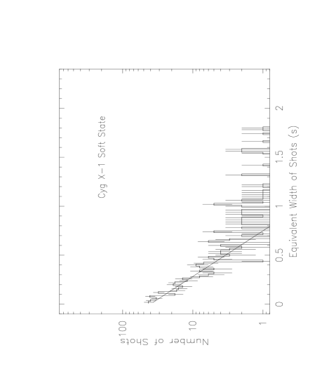
Figure 6: Same as figure 5, but the data are for the 1996 July (soft state) observations. The exponential fit has a time constant of 0.2 s.

A similar shot statistics is shown in Figure 6 for the soft state observations. The distribution is much steeper with an e-folding constant of 0.2 s. Apart from this, there are a large number of high intensity shots over and above that described by the exponential function. We have also generated the shot distribution for the soft state when the count rates are taken in 0.1 s bins (Figure 7). The distribution is steep with an e-folding constant of 0.04 s. We also find a shot with large excess counts (with an equivalent width of 0.92 s). The formal probability that this shot occurred at random assuming a shot occurrence rate described by an exponential function is 2 $\times$ 10^-7. This shot was detected by PPC-1 on 1996 July 5. The light curve for this shot is shown in Figure 8 for the total counts (top panel), 2-6 keV counts (middle panel) and 6-18 keV counts (bottom panel). The shot can be described by exponential rise and decays with a time constant of 0.4 s.

The shot width distribution also shows an exponential distribution. We find that in the hard state it has a time constant of 1.4 s, and the distribution becomes flatter in the soft state with a time constant of 2.2 s. We also find that the distribution cannot be described by other simple functional forms like power-law etc.

4 Discussion

Detailed observations of Cyg X-1 made using the PCA on-board the RXTE (Cui et al., 1997a,b; Belloni et al., 1996) have shown that the power density spectrum (PDS) of the source changes smoothly during the spectral transition from the hard state to the soft state and reverts back when there is a transition back to the hard state. The power-law index for the PDS below 0.3 Hz for the transition state was found to be between -0.3 to -0.7. The observations carried out by the PPCs in 1996 May pertain to the hard state of the source, where there were no PCA observations. We find that the index is still flatter in the hard state, about -0.09, and the PDS shape agrees very well with the traditional hard state PDS obtained earlier (Belloni & Hasinger 1990a). These observations reinforce the conclusion obtained by Cui et al. that the changes in the PDS smoothly follow the spectral changes.

Chakrabarti & Titarchuk (1995) have worked out a complete solution of viscous transonic equations and have identified the various X-ray emission regions in an accretion disk. Here we attempt to identify the different components in the PDS with the different regions of the accretion disk as described by Chakrabarti & Titarchuk (1985). Most of the white noise component in the PDS can originate in the post-shock region. In the soft state, the Compton cooling is very efficient resulting in bulk motions which can lead to much higher red noise in the PDS. The very low frequency component in the PDS (at $<$0.01 Hz) identified in the present work appears to be independent of the spectral states. The origin of this component could be from the pre-shock sub-Keplerian component.

The distribution of shots in Cyg X-1 has been explained under the premises of self-organized criticality (SOC) model (Mineshige et al. 1994a). Negoro et al. (1995) have examined this model by analyzing the Ginga data for the hard state of Cyg X-1. They have also put a selection criterion for shots, namely, the shot peak count rates should be higher than the running average by a pre-determined factor, p. It was found that the shot widths follow an exponential distribution with time constants of 1.8 s, 8.4 s and 23.8 s for values of p 1.5, 2 and 2.35, respectively. For our analysis, we have taken all shots (p is 1) and find that the shot width has an exponential distribution with time constant of 1.4 s. This value appears to be consistent with 1.8 s (for p $=$ 1.8), since the time constant decreases with decreasing p. The important conclusion that can be drawn from our work is that the shot width as well as the total shot intensity has an exponential distribution in both the spectral states. The distinct change in the shot distribution for the two spectral states is a new input for the shot modeling and it probably indicates the differences in the basic model parameters like the critical mass density, diffusion coefficient etc.

The large shot detected in our work appears similar to the shape of the co-added shots obtained from the Ginga data (Negoro et al. 1994). They have found two time constants each for the rise and decay phase of values 0.1 and 1 s, respectively. The value obtained in the present work (0.4 s) lies in between these two values.

5 Conclusions

We have analyzed the data obtained from the Indian X-ray Astronomy Experiment (IXAE) on Cyg X-1 in its two spectral states. A method is evolved for background subtraction. The timing analysis has shown that:

1. The power density spectrum (PDS) shows substantial differences in the two spectral states: the power-law index between 0.03 to 0.3 Hz changed from -0.09 to -1.02 when the source changed from the hard to the soft state.

2. A new component in the PDS below 0.03 Hz has been identified and this component appears to be independent of the spectral state.

3. The shot statistics like the duration and the energy in shots show exponential distribution and the time constant shows significant difference in the two spectral states.

4. A large individual shot has been identified and it has an exponential rise and decay with a time constant of 0.4 s.

Table 1: Log of observation

Observation	Cyg X-1	Time	Live	time	(sec)	Observed	flux	(mCrab)
date	binary	resolution	PPC-1	PPC-2	PPC-3	PPC-1	PPC-2	PPC-3
time	phase	(sec)
Apr 30 12:10	.44	1.0	–	895	697	–	503	514
Apr 30 13:50	.45	1.0	–	898	897	–	434	437
May 1 11:48	.61	1.0	–	–	696	–	–	633
May 1 13:30	.63	1.0	–	–	800	–	–	562
May 1 15:10	.64	1.0	–	–	896	–	–	573
May 3 11:05	.97	1.0	799	800	–	431	417	–
May 3 12:46	.98	1.0	795	899	–	395	384	–
May 3 14:28	.99	1.0	696	699	–	398	383	–
May 3 23:43	.06	1.0	694	–	699	437	–	471
May 4 04:58	.10	time-tagged	338	–	338	396	–	420
May 9 06:28	.00	1.0	477	675	500	319	308	356
May 9 14:03	.06	1.0	–	900	898	–	437	445
May 9 23:18	.13	1.0	700	698	697	390	384	390
May 10 00:58	.14	1.0	800	797	800	365	354	365
May 10 02:38	.15	1.0	899	896	900	364	346	379
May 10 06:03	.18	1.0	695	–	799	362	–	363
May 10 13:45	.24	1.0	628	–	644	449	–	439
May 10 15:23	.25	1.0	499	–	499	430	–	422
May 10 17:09	.27	time-tagged	1085	–	1085	308	–	298
May 10 22:58	.30	1.0	599	601	597	418	386	440
May 11 00:36	.32	1.0	799	797	796	430	385	455
May 11 02:16	.33	1.0	897	995	–	337	283	–
Jul 5 14:21	.24	0.1	700	–	–	756	–	–
Jul 8 13:16	.77	0.1	800	900	–	773	857	–
Jul 8 15:07	.79	0.1	251	335	–	939	1079	–

Figure 1: The observed background counts in PPC2r top layer are plotted against the ULD (upper level discriminator) counts, which is a measure of the particle background. The integration time for the data points is 100 s. The continuous line in the figure is a least square straight line fit.

Figure 2: The background subtracted count rates from PPC-2 obtained during the hard state of Cyg X-1 (1996 May) are shown in the top panel. Count rates from the same detector obtained in 1996 July (during the soft state of Cyg X-1) are shown in the bottom panel. The time resolution is 1 s. The start time is arbitrary.

Figure 3: The power density spectrum (PDS) for the hard state of Cyg X-1 obtained during 1996 May from the PPC observations as well as from the ASM data.

Figure 4: Same as figure 3, but the data are for the 1996 July (soft state) observations.

Figure 5: The Shot statistics of Cyg X-1 for the hard state (1996 May) observations. The total number of shots of a given total excess counts (normalized to the local mean) are plotted against the excess counts (differential plot). The units of the excess counts are equivalent width in seconds. The best fit exponential function is shown as a straight line, and the derived time constant is 0.35 s. Time resolution of the light curve used for generating shot statistics is 1s.

Figure 7: Same as figure 6, but the time resolution for the flare statistics generation is 0.1 s. The exponential fit has a time constant of 0.04 s.

Figure 8: The details of the largest shot observed during the soft state (1996 July). The observed counts per bin (for a bin size of 0.1 s) are shown for PPC-1 total counts (top panel), 2 keV $-$ 6 keV counts (middle panel) and 6 keV $-$ 18 keV counts (bottom panel). The time is given in seconds starting from 1996 July 5 14:21 UT.

References

- (1) Agrawal, P.C., Paul, B., Rao, A.R. et al., 1996, J. Korean Astron. Soc., 29, S429.
- (2) Agrawal, P.C. et al., 1997, in preparation.
- (3) Belloni, T., Hasinger, G., 1990a, A&A, 227, L33.
- (4) Belloni, T., Hasinger, G., 1990b, A&A, 230, 103.
- (5) Belloni, T., Mendez, M., van der Klis, M., Hasinger, G., Lewin, W.H.G., van Paradijs, J., 1996, ApJ, 472, L107
- (6) Chakrabarti, S.K., and Titarchuk, L.G., 1995, ApJ, 455, 623.
- (7) Chitnis, V.R., Rao, A.R., Agrawal, P.C., 1997, A&A, submitted.
- (8) Cui, W., 1996, IAUC 6404.
- (9) Cui, W., Heindl, W.A., Rothschild, R.E., Zhang, S.N., Jahoda, F., Focke, W., 1997a, ApJ, 474, L57
- (10) Cui, W., Zhang, S.N., Focke, W., Swank, J.H., 1997b, ApJ, in press.
- (11) Gierlinski, M., Zdziarski, A. A., Done, C., Johnson, W. N., Ebisawa, K., Ueda, Y., Haardt, F., Phlips, B., 1997, MNRAS, 288, 958.
- (12) Gies, D.R. and Bolton, C.T., 1982, ApJ, 260, 240.
- (13) Liang, E.P. and Nolan P.L., 1984, Space Sci. Rev., 38, 353.
- (14) Lochner, J.C., Swank, J.H., Szymkowiak, A.E., 1991, ApJ, 375, 295
- (15) McIlwain, C.E., 1977, JGR, 66, 3681
- (16) Mineshige, S., Ouchi, N.B., Nishimori, H., 1994a, PASJ, 46, 97
- (17) Mineshige, S., Takeuchi, M., Nishimori, H., 1994b, ApJ, 435, L128
- (18) Misra, R., Chitnis, V.R., Melia, F., Rao, A.R., 1997, ApJ, in press.
- (19) Miyamoto, S., Kitamoto, S., 1989, Nat, 342, 773
- (20) Molteni, D., Sponholz, H. and Chakrabarti, S. K., 1996, ApJ 457, 805
- (21) Narayan, R., Yi, I., 1994, ApJ, 428, L13
- (22) Negoro, H., Miyamoto, S., Kitamoto, S., 1994, ApJ, 423, L127
- (23) Negoro, H., Kitamoto, S., Takeuchi, M., Mineshige, S., 1995, ApJ, 452, L49
- (24) Nolan, P.L., Bruber, D.E., Matteson, J.L., Peterson, L.E., Rothschild, R.E., Doty, J.P., Levine, A.M., Lewin, W.H.G., Primini, F.A., 1981, ApJ, 246, 494.
- (25) Oda, M., 1977, Space Sci. Rev. 20, 757
- (26) Weisskopf, M.C., Sutherland, P.G., Katz, J.I., Canizares, C.R., 1978, ApJ, 233, L17
- (27) Zhang, S.N., Harman, B.A., Paciesas, W.S., 1996, IAUC 6447