The Ocean and Crust of a Rapidly Accreting Neutron Star: Implications for Magnetic Field Evolution and Thermonuclear Flashes

Abstract

We investigate the atmospheres, oceans, and crusts of neutron stars accreting at rates sufficiently high (typically in excess of the local Eddington limit) to stabilize the burning of accreted hydrogen and helium. For hydrogen-rich accretion at global rates in excess of $10^{-8}M_{\odot}\,{\rm yr}^{-1}$ (typical of a few neutron stars), we discuss the thermal state of the deep ocean and crust and their coupling to the neutron star core, which is heated by conduction (from the crust) and cooled by neutrino emission. We estimate the Ohmic diffusion time in the hot, deep crust and find that it is noticeably shortened (to less than $10^{8}\,{\rm yr}$) from the values characteristic of the colder crusts in slowly accreting neutron stars. As suggested by Konar & Bhattacharya, at high accretion rates the flow timescale competes with the Ohmic diffusion time in determining the evolution of the crust magnetic field. At a global accretion rate of $\dot{M}\approx 3\times 10^{-9}M_{\odot}\,{\rm yr}^{-1}$, the Ohmic diffusion time across a scale height equals the flow time over a large range of densities in the outer crust. In the inner crust (below neutron drip), the diffusion time is always longer than the flow time, for sub-Eddington accretion rates. We speculate on the implications of these calculations for magnetic field evolution in the bright accreting X-ray sources.

We also explore the consequences of rapid compression at local accretion rates exceeding ten times the Eddington rate. This rapid accretion heats the atmosphere/ocean to temperatures of order $10^{9}\,{\rm K}$ at relatively low densities; for stars accreting pure helium, this causes unstable ignition of the ashes (mostly carbon) resulting from stable helium burning. This unstable burning can recur on timescales as short as hours to days, and might be the cause of some flares on helium accreting pulsars, in particular 4U 1626–67. Such rapid local accretion rates are common on accreting X-ray pulsars, where the magnetic field focuses the accretion flow onto a small fraction of the stellar area. We estimate how large such a confined “mountain” could be, and show that the currents needed to confine the mountain are large enough to modify, by order unity, the magnetic field strength at the polar cap. If the mountain’s structure varies in time, the changing surface field could cause temporal changes in the pulse profiles and cyclotron line energies of accreting X-ray pulsars.

To appear in the Astrophysical Journal, 1 April 1998

1 Introduction

The thermal and compositional structure of the outer layers of an accreting neutron star is of interest to studies of accretion-induced magnetic field decay (e.g., [Urpin & Geppert 1995]), thermonuclear processes, and the thermal and compositional structure of the inner crust and core. In this paper, we consider objects accreting at rates high enough for stable burning of hydrogen and helium (typically requiring super-Eddington rates; for a recent review see Bildsten 1998) and examine the thermal and compositional structure of the underlying ocean and crust. By “ocean and crust” we mean the region far below where the accreted matter is decelerated from its free-fall velocity and directly underneath the hydrogen/helium burning layer (Fig. 1 provides a sectional cut through this part of the neutron star). We are therefore considering fluid layers that are gradually being compressed by the continuous addition of fluid at the top of the atmosphere. Previous works ([Ayasli & Joss 1982]; [Fujimoto et al. 1984]; [Miralda-Escudé et al. 1990]) have examined this problem for stars accreting at globally sub-Eddington rates in a spherically symmetrical fashion. In this paper, we do not impose such a restriction and therefore parameterize accretion by the local rate per unit area, $\dot{m}$. In general, neutron stars accrete at super-Eddington rates by means of an optically thick column; on accretion-powered X-ray pulsars, the local accretion rate in this column can easily exceed the Eddington rate by orders of magnitude.

Our motivation is twofold. For hydrogen-rich accretion at global rates of order $10^{-8}M_{\odot}\,{\rm yr}^{-1}$ (the Eddington limit), we find the minimum temperature in the deep crust and the resulting maximum possible Ohmic diffusion time there. This is applicable to the brightest accreting objects in our galaxy (e.g. Sco X-1 and the GX objects, which are weakly magnetic, $B\ll 10^{12}\,{\rm G}$) and the Magellanic Clouds. For accreting pulsars with high magnetic fields ($\gtrsim 10^{12}\,{\rm G}$), we mostly consider the conditions underneath the accreting polar cap, where magnetic confinement of the accreted matter ensures a locally high accretion rate that rapidly compresses the ocean and heats it to temperatures of order $10^{9}\,{\rm K}$ at low densities. If this accreted matter contains an appreciable amount of carbon (or oxygen), a violent thermonuclear instability occurs and produces a flare from the polar cap. At super-Eddington local accretion rates, the recurrence time for this instability is short enough (hours to days) to allow observations of the flares.

Figure 1: Schematic of the outer layers of an accreting neutron star. Infalling matter (straight arrows) is decelerated from a velocity $v\sim 0.5c$ at a shock and radiates a flux $F\approx GM\dot{m}/R$. Beneath the shock, the accreted matter forms an atmosphere/ocean in hydrostatic balance where the downward flow velocity is $v=\dot{m}/\rho$ (§ 2). We indicate both the density and the physical depth (roughly the pressure scale height) of the underlying layers on the left-hand side of the diagram. The flux (wavy arrows) in this region is set by the steady-state hydrogen and helium burning {here $E_{\rm nuc}=X[(Q_{H}/4)+(Q_{3\alpha}/12)]+Y(Q_{3\alpha}/12)$, see eq. [12]}. Below the H/He burning region, the matter forms an electron-degenerate ocean (§ 4), where energy transport is mediated by electron conduction. The ocean is nearly isothermal, and the flux is set by further compression of the matter (see eq. [24]). At a density of roughly $10^{9}\,{\rm g}\,{\rm cm}^{-3}$, the ions crystallize into a lattice. The thermal state of the crust and core is described in § 4.3.

We start in § 2 by deriving the Eulerian fluid equations for a plane-parallel geometry. Presuming steady-state hydrogen/helium burning (valid for super-Eddington accretion), we briefly investigate, in § 3, the thermal structure of the star’s upper atmosphere. Because the case of pure helium accretion is simpler, and because it is relevant to a number of binaries, we first study the steady-state burning of helium and show that the ashes of this burning are mostly carbon. When the neutron star is accreting a hydrogen-rich mixture at approximately the Eddington rate, the stable hydrogen burning is never fast enough to consume all of the hydrogen before the helium ignites. Rapid proton captures onto the rapidly proliferating seed nuclei then produce a mix of heavy (trans-iron) elements. Although the final mix is quite complicated (and has yet to be calculated), the thermal profile is readily found.

We next move down to the degenerate electron ocean, where the density is greater than $10^{6}\,{\rm g}\,{\rm cm}^{-3}$. The thermal flux flowing through the ocean is mostly generated by settling and compression within it. We show in § 4 how $\dot{m}$ determines the thermal profile of this deep ocean. Non-equilibrium nuclear reactions (mostly neutron emissions and pycnonuclear reactions) are an important heat source in the deep crust ([Haensel & Zdunik 1990]). Using a crude formulation of the crust heat sources, we show that most of this energy is conducted into the neutron star core, which finds a steady-state core temperature hot enough to balance this heating with neutrino losses.

In § 5, we use the thermal profiles in the crust to estimate the Ohmic diffusion time there. The effect of accretion-induced heating on the Ohmic decay of crust magnetic fields has previously been considered ([Romani 1990]; [Geppert & Urpin 1994]; [Pethick & Sahrling 1995]; [Urpin & Geppert 1995]; [Urpin & Geppert 1996]; [Konar & Bhattacharya 1997]) for stars accreting at sub-Eddington rates. In the deep crust, the local accretion rate is roughly independent of latitude; there are, however, a few systems that accrete globally at or near the Eddington rate. As a first cut, we compute the Ohmic diffusion time across a scale height throughout the outer crust ($\rho\lesssim 10^{13}\,{\rm g}\,{\rm cm}^{-3}$) and find that it is greater than the time for matter to flow across a scale height for near-Eddington accretion rates. This implies that crust magnetic fields are advected to great depths before they are able to decay.

Although variations with latitude in the local accretion rate may be negligible deep within the crust, they cannot be ignored in the upper ocean and atmosphere. In the case of accretion-powered pulsars, for which the infalling accretion stream is funneled onto a small area about the polar cap, the local accretion rate can be very super-Eddington even if the global accretion rate is sub-Eddington. The lack of type I X-ray bursts implies a locally super-Eddington accretion rate at the cap in accreting pulsars (Joss & Li 1980; Ayasli & Joss 1982; Bildsten & Brown 1997). In § 6, we show that the matter is tied to the field lines to very large depths and that spreading away from the polar cap does not occur until the accreted matter reaches pressures greatly exceeding $B^{2}/8\pi$ (a detailed discussion is in Appendix B). The resulting high local accretion rate causes unstable carbon ignition at relatively low densities (§ 7). The low ignition column depth and rapid accretion rate combine to make the resulting large “flares” from the polar caps recur on an hourly to daily timescale. This timescale differs strongly with the calculation of Woosley & Taam (1976), who found a roughly ten yr recurrence time for near-Eddington accretion rates. We discuss the observable signatures of such burning, and briefly compare our theoretical models to some accreting X-ray pulsars, including LMC X-4 and 4U 1626–67. We conclude in § 8 with a summary of our main results.

2 The Equations in Planar Geometry

Because the accretion flow onto the neutron star is in general asymmetrical, we define a local accretion rate, $\dot{m}$, as the mass accreted per unit time per unit area. The physics of the reactions, compression, and settling all depend on this quantity. The local Eddington accretion rate is

$$\dot{m}_{\rm Edd}=\frac{\mu_{e}m_{u}c}{\sigma_{T}R}=7.5\times 10^{4}\,{\rm g}\,{\rm cm}^{-2}\,{\rm s}^{-1}\mu_{e}\left(\frac{R}{10\,{\rm km}}\right)^{-1},$$ (1)

where $\sigma_{T}$ is the Thomson scattering cross-section, $c$ is the speed of light, $R$ is the radius of the star, $m_{u}$ is the atomic mass unit, and the number density of electrons is $\rho/(\mu_{e}m_{u})$. Future references to $\dot{m}_{\rm Edd}$ are for $\mu_{e}=1$. Because the ram pressure in the internal sub-sonic flow is negligible, the momentum equation is just that of hydrostatic balance,

$$\frac{dP}{dz}=-\rho g,$$ (2)

allowing us to parameterize the spatial coordinate by column depth, $y(z)\equiv\int_{z}^{\infty}\rho\,dz^{\prime}$, so that $P(z)=gy(z)$. The heat flux flowing through the deep atmosphere (far beneath the photosphere, see Fig. 1) is much less than the accretion flux ($\approx G\dot{M}m_{u}/R$), so radiation pressure is unimportant. Since accretion does not appreciably change the radial coordinate of isobars (see Appendix A), $y$ is an Eulerian coordinate. We take the surface gravity $g$ to be constant, since the pressure scale height, $H=P/\rho g$, is much less than $R$ everywhere in the atmosphere. Throughout this paper, we assume a neutron star mass and radius of $1.4M_{\odot}$ and $10\,{\rm km}$, respectively; we also use Euclidean spacetime, with $g=GM/R^{2}$. We ignore components of heat transport and pressure gradients parallel to the surface. Even in the case of accretion onto a small fraction of the surface, the atmospheric scale height is much smaller than lengthscales along the surface. As a result, the area of the top and bottom “faces” of the ocean under the accretion column is much greater than the area along the “edges”. For a polar cap of radius $10^{5}\,{\rm cm}$ (a tenth of the stellar radius), the ratio of edge area to face area is $\sim 10^{-2}$.

The continuous accretion of fresh material modifies the equations of continuity and entropy. The continuity equation for a species $j$ (with number density $n_{j}$) is

$$\frac{\partial n_{j}}{\partial t}+\mbox{\boldmath$\displaystyle\nabla$}\mbox{\boldmath$\displaystyle\cdot$}\,(n_{j}\mbox{\boldmath$\displaystyle v$})=-r_{\rm dest}^{(j)}+r_{\rm prod}^{(j)},$$ (3)

where $r_{\rm dest}^{(j)}$ ($r_{\rm prod}^{(j)}$) is the destruction (production) rate of species $j$ due to thermonuclear reactions. We presume that all ions co-move (a good approximation at high accretion rates where the downward compression is faster than any drift time for a heavy particle). Defining a mass fraction

$$X_{j}\equiv\frac{\rho_{j}}{\rho}=\frac{A_{j}m_{u}n_{j}}{\rho},$$ (4)

where $A_{j}$ is the baryon number of species $j$, and, recognizing that the accreted matter flows through constant pressure surfaces at a velocity $v=\dot{m}/\rho$, we expand the continuity equation (eq. [3]) in $(y,t)$ coordinates to obtain

$$\frac{\partial X_{j}}{\partial t}+\dot{m}\frac{\partial X_{j}}{\partial y}=\frac{A_{j}m_{u}}{\rho}(-r_{\rm dest}^{(j)}+r_{\rm prod}^{(j)}).$$ (5)

In this derivation we neglect the contribution of binding energy to $\rho$. The entropy equation is

$$T\frac{ds}{dt}=-\frac{1}{\rho}\mbox{\boldmath$\displaystyle\nabla$}\mbox{\boldmath$\displaystyle\cdot$}\,\mbox{\boldmath$\displaystyle F$}+\epsilon,$$ (6)

where $\displaystyle F$ is the flux and $\epsilon$ is the sum of all sources and sinks of entropy. The flux obeys Fick’s law,

$$\mbox{\boldmath$\displaystyle F$}=-K\mbox{\boldmath$\displaystyle\nabla$}T,$$ (7)

with $K$ denoting the thermal conductivity. Heat transport is set by both radiative (primarily Thomson scattering and free-free absorption) and conductive (electron-electron and electron-ion scattering) processes. The total thermal conductivity is then

$$K=\frac{4ac}{3\rho\kappa_{\rm rad}}T^{3}+K(\mbox{\rm conduction}),$$ (8)

where $\kappa_{\rm rad}$ is the radiative opacity. Using the equations for hydrostatic balance (eq. [2]) and flow velocity $v=\dot{m}/\rho$, and the thermodynamic relation

$$\left(\frac{\partial s}{\partial P}\right)_{T}=-\left(\frac{\partial T}{\partial P}\right)_{s}\left(\frac{\partial s}{\partial T}\right)_{P},$$ (9)

we write the entropy as a function $s=s(T(y,t),P(y))$ and transform equations (6) and (7) into the more useful forms

$$\frac{\partial F}{\partial y}+\epsilon = c_{\!P}\left(\frac{\partial T}{\partial t}+\dot{m}\frac{\partial T}{\partial y}\right)-\frac{c_{\!P}T\dot{m}}{y}\nabla_{\rm\!ad}$$ (10)

$$\frac{\partial T}{\partial y} = \frac{F}{\rho K}.$$ (11)

Here $c_{\!P}$ is the specific heat at constant pressure, and $\nabla_{\rm\!ad}\equiv(\partial\ln T/\partial\ln P)_{s}$ is the adiabat. Equations (5), (10), and (11) with appropriate boundary conditions describe the thermal evolution of the outer layers of the neutron star.

3 Hydrogen and Helium Burning in the Upper Atmosphere

We now derive the thermal and compositional state of the upper atmosphere for these characteristically high accretion rates. This determines the outer starting point for the derivation of the conditions deeper in the ocean and crust. The accreting hydrogen and helium typically fuse to heavier elements within an hour after arrival at the neutron star atmosphere. Because of $\beta$-decay limitations, hydrogen burning via the CNO cycle is stable at $\dot{m}\gtrsim 10^{-2}\dot{m}_{\rm Edd}$ and never fast enough to consume the accreting hydrogen before the helium ignites ([Lamb & Lamb 1978]; [Taam & Picklum 1979]; Fujimoto, Hanawa, & Miyaji 1981). For $\dot{m}\gtrsim 10^{-1}\dot{m}_{\rm Edd}$, helium burning occurs in a hydrogen-rich environment, which enhances the nuclear reaction chains and energy release (Taam 1982, 1985). All analyses ([Joss & Li 1980]; [Ayasli & Joss 1982]; [Fushiki & Lamb 1987b]; Taam, Woosley, & Lamb 1996) have shown that the helium burning in this mixed environment becomes thermally stable when the local accretion rate is, by coincidence, super-Eddington (see Bildsten 1998 for a review). It is in this stable regime that we carry out our calculations.

Finding the compositional makeup of the ashes from steady-state hydrogen-rich accretion is complicated by the rp-process ([Wallace & Woosley 1981]; [Champagne & Wiescher 1992]; [Van Wormer et al. 1994]; [Schatz et al. 1998]), a sequence of rapid proton captures onto nuclei that can produce proton-rich elements beyond iron. The energy released is approximately known, however, so that we can roughly determine the upper atmosphere’s thermal profile for steady-state burning. Before discussing this problem, we first consider the simpler case of pure helium accretion. This is relevant to a number of ultra-compact ($P_{\rm orb}<50{\rm\,min}$) binaries (4U 1626–67, 4U 1820–30, and 4U 1916–05, Nelson, Rappaport, & Joss 1986; potentially X1850–087, [Homer et al. 1996]) and maybe the wide binary Cygnus X-3, if it in fact contains a neutron star.

3.1 Steady-State Pure Helium Burning

There are a few neutron stars thought to be accreting nearly pure helium. For these stars, the first nuclear reaction is $\rm 3\alpha\rightarrow{}^{12}C$. We use the energy generation rate from Fushiki & Lamb (1987a) where $Q_{3\alpha}=7.274\,{\rm MeV}$ is the energy released per formed carbon. The radiative opacity $\kappa_{\rm rad}$ is the sum of electron scattering (with high temperature and degeneracy corrections from Paczyński 1983) and free-free absorption. We use the conductive opacity, $\kappa_{\rm cond}=3\rho K({\rm conductive})/4acT^{3}$, as given by Fushiki (1986). The degenerate electron pressure is calculated using an interpolation formula from Paczyński (1983).

The density at the location of helium burning decreases as the accretion rate increases, which eventually allows the $\rm{}^{12}C$$\rm\,(\alpha,\gamma)\,$$\rm{}^{16}O$ reaction to compete with the $3\alpha$ reaction in consuming helium. We use Buchmann’s (1996) reaction rate with the fitting formula that yields $S=146\,{\rm keV}{\rm\,barns}$ at 300 keV center-of-mass energy. This rate is roughly 1.7 times the Caughlan & Fowler (1988) $\rm{}^{12}C$$\rm\,(\alpha,\gamma)\,$$\rm{}^{16}O$ rate, and so is more consistent with nucleosynthetic constraints ([Weaver & Woosley 1993]). Recent measurements ([Azuma et al. 1994]) also support this S-factor value. In addition to $\rm{}^{12}C$$\rm\,(\alpha,\gamma)\,$$\rm{}^{16}O$, we also include the subsequent $\rm{}^{16}O$$\rm\,(\alpha,\gamma)\,$$\rm{}^{20}Ne$, $\rm{}^{20}Ne$$\rm\,(\alpha,\gamma)\,$$\rm{}^{24}Mg$, and $\rm{}^{24}Mg$$\rm\,(\alpha,\gamma)\,$$\rm{}^{28}Si$ reactions. The reaction $\rm{}^{28}Si$$\rm\,(\alpha,\gamma)\,$$\rm{}^{32}S$ is unimportant for $\dot{m}\leq 40\,\dot{m}_{\rm Edd}$, although for higher rates the reaction network would have to include it as well. For these reactions, we use rates from Caughlan & Fowler (1988) with the following adjustments: (1) following Schmalbrock et al. (1983), we set the uncertain factor between 0 and 1 in the $\rm{}^{20}Ne$$\rm\,(\alpha,\gamma)\,$$\rm{}^{24}Mg$ rate to 0.1; (2) we also set the uncertain factor between 0 and 1 in the $\rm{}^{24}Mg$$\rm\,(\alpha,\gamma)\,$$\rm{}^{28}Si$ rates to 0.1. Screening is treated according to Salpeter & Van Horn (1969).

We simultaneously integrate the steady-state versions of the continuity, flux, and entropy equations (eqs. [5], [11], [10]) as a function of column depth. Our integration starts far beneath the photosphere, where the outward heat flux is set by the energy released from nuclear reactions and the settling of the material. Though the flux coming through the envelope is much less than the accretion flux ($\approx GM\dot{m}/R$), the temperature just beneath the photosphere is still near the value set by the accretion flux. The flux at the top of the atmosphere would simply be $F=(Q_{3\alpha}/12m_{u})\dot{m}=0.61\,{\rm MeV}(\dot{m}/m_{u})$ if all the helium burned to carbon and there was no energy released from gravitational settling. However, we are interested in the makeup of the products of helium burning; moreover, the heat released from gravitational settling is non-negligible at high accretion rates. A hotter atmosphere has a greater scale height, and so at high accretion rates more energy is released by lowering a parcel of fluid a distance of order a scale height. To integrate the fluid equations, we start with a trial value of the flux and integrate equations (10) and (11) to the depth where all the helium is burned. At this point, we compare the flux to that coming from further gravitational settling of the ashes (see § 4) in deeper regions of the star, and iteratively adjust the flux.

Figure 2: Atmospheric temperature and composition for steady-state accretion and burning of pure helium. The neutron star is of mass $M=1.4M_{\odot}$ and radius $R=10^{6}\,{\rm cm}$, and the accretion rate is $\dot{m}=10.0\,\dot{m}_{\rm Edd}=7.5\times 10^{5}\,{\rm g}\,{\rm cm}^{-2}\,{\rm s}^{-1}$. The temperature is shown by the solid line in the top panel, whereas the dashed line displays the outward directed flux per accreted baryon. The bottom panel displays the mass fractions of the major elements present ($\rm{}^{12}C$, $\rm{}^{16}O$, $\rm{}^{20}Ne$, $\rm{}^{24}Mg$, and $\rm{}^{28}Si$) for pure helium burning.

When burning in steady-state, the helium is consumed at the column depth $y$ where its lifetime to the $3\alpha$ reaction is the time to reach that depth, $t_{\rm fl}\approx y/\dot{m}$. For the values of $\dot{m}$ considered here, burning occurs at a column depth $y\approx 10^{8}\,{\rm g}\,{\rm cm}^{-2}$, which is reached in a time $t_{\rm fl}<10^{3}$ seconds. Bildsten (1998) provides a simple discussion of the physics of the thermal stability of helium burning. Linear perturbation calculations show that the helium burning is thermally unstable when $T<5\times 10^{8}\,{\rm K}$ in the burning region (Bildsten 1995, 1998). From our steady-state calculations and a few time-dependent calculations, as in Bildsten (1995), we find that pure helium burning is thermally unstable until $\dot{m}\gtrsim 10\,\dot{m}_{\rm Edd}$.

Figures 2, 3, and 4 display the steady-state thermal and compositional structure of the outer layers of the neutron star accreting helium at rates of $\dot{m}/\dot{m}_{\rm Edd}=10$, 20, and 40, respectively. Each figure shows the results for a different accretion rate. The top panel displays the temperature (solid line) and the flux per baryonic accretion rate, $F/(\dot{m}/m_{u})$ (dashed line). The flux flowing through the atmosphere increases with $\dot{m}$; this leads to increasingly hotter temperatures and lower densities at the location of the burning and subsequently more contributions from the $\alpha$ captures on carbon. For each of Figures 2, 3, and 4, the composition as a function of column depth is shown in the bottom panel. As we show in Figure 4, at $\dot{m}=40\,\dot{m}_{\rm Edd}$ the final mixture is $\frac{2}{3}$ carbon and $\frac{1}{3}$ silicon. At lower accretion rates, the dominant nucleus made from helium burning is carbon. The outward-directed flux at the bottom of the atmosphere comes from the gravitational settling of matter beneath the helium burning region. This flux is determined by continuing the integration of equations (10) and (11) to very deep parts of the neutron star, as described in section 4.

Figure 3: Same as Fig. 2, but for an accretion rate $\dot{m}=20.0\,\dot{m}_{\rm Edd}=1.5\times 10^{6}\,{\rm g}\,{\rm cm}^{-2}\,{\rm s}^{-1}$.

3.2 Steady-State Burning of Accreting Hydrogen and Helium

At these high accretion rates, the hydrogen cannot burn rapidly enough to be depleted prior to helium ignition. As a result, hydrogen burning proceeds via the rp-process, which is accelerated by the proliferation of “seed” nuclei from helium burning. As a first guess, we presume that the hydrogen burns completely where the helium ignites and neglect calculating the composition of the ashes. These atmospheres are much hotter than the pure helium burning case (for the same $\dot{m}$) due to the larger flux flowing through the envelope; this leads to thermally stable helium burning once $\dot{m}\gtrsim\dot{m}_{\rm Edd}$ ([Bildsten 1998]).

We presume that the flux flowing through the atmosphere is that released from burning all of the hydrogen and helium to carbon,

$$F=\frac{\dot{m}}{m_{u}}\left[X\left(\frac{Q_{H}}{4}+\frac{Q_{3\alpha}}{12}\right)+Y\frac{Q_{3\alpha}}{12}\right],$$ (12)

where $Q_{H}=28\,{\rm MeV}$ is the energy release per formed helium. This approximation yields lower limits to the true temperature at the location of helium burning in the presence of the more complex rp-process for two reasons. First, we presume that the reactions proceed only to carbon, although the residual nuclei are likely to be much heavier. In addition, Taam et al. (1996) have found (for high accretion rate type I bursts) that not all of the hydrogen is consumed at the location where the helium is depleted, in which case there is further energy release from electron capture on protons at larger depths in the atmosphere (for a recent discussion, see [Bildsten & Cumming 1998]). Therefore, our thermal profiles for depths greater than where helium burns should be considered as lower limits.

Figure 4: Same as Fig. 2, but for an accretion rate $\dot{m}=40.0\,\dot{m}_{\rm Edd}=3.0\times 10^{6}\,{\rm g}\,{\rm cm}^{-2}\,{\rm s}^{-1}$.

For accretion rates $\dot{m}/\dot{m}_{\rm Edd}=1.0$, 5.0, 10.0, and 20.0 and a helium fraction $Y=0.3$ (Fig. 5), we integrate equation (11), with the flux given by equation (12), downwards into the atmosphere until one-half of the incident helium has burned. At this point, we presume that all the hydrogen has burned as well, in which case the flux originating from deeper points is entirely caused by gravitational settling. For definiteness, we took the composition to be either carbon (solid curve) or iron (dotted curve). The helium ignition depth (clearly denoted by the discontinuity in slope) is nearly independent of the accretion rate, yielding times to helium ignition of roughly $0.4\,(\dot{m}_{\rm Edd}/\dot{m}){\rm\,hr}$. At the highest accretion rate shown, the infalling helium ignites only 80 s after arrival onto the neutron star. The helium burning is stable once $\dot{m}\gtrsim\dot{m}_{\rm Edd}$; the cooling rate at the temperature ($5\times 10^{8}\,{\rm K}$) in the helium burning region at that accretion rate is fast enough to stabilize the burning.

Figure 5: Atmospheric temperature profiles for hydrogen-rich accretion ($X=0.7,\ Y=0.3$) at the super-Eddington accretion rates (from bottom to top) $\dot{m}/\dot{m}_{\rm Edd}=1$, 5, 10, and 20. In the outer atmosphere, the flux is set by hydrogen/helium burning (dot-dashed curves). Where the helium is half-depleted, we join these curves onto the settling solutions (no burning) for an ocean of either carbon (solid curves) or iron (dotted curves). The slopes are discontinuous at this point because the flux released from settling and compression alone is much less than the burning flux. If any carbon is present, it will ignite where $d\epsilon_{\rm nuc}/dT=d\epsilon_{\rm cool}/dT$ (see § 7.1; heavy dashed line). The iron settling solutions end at a lower column depth than the carbon settling solutions because of crystallization. At column depths greater than $\sim 10^{9}\,{\rm g}\,{\rm cm}^{-2}$, the density is approximately given by eq. (19).

4 Gravitational Compression of the Ashes in the Deep Ocean

We now discuss the thermal state of the degenerate ocean underneath the hydrogen/helium burning region. Upon completion of stable hydrogen/helium burning, the gas is hotter than $5\times 10^{8}\,{\rm K}$ and denser than $(\mbox{2--5})\times 10^{5}\,{\rm g}\,{\rm cm}^{-3}$. The temperature and nuclear evolution of this matter under further compression depends on both the local accretion rate and the composition.

First consider steady-state settling solutions in the absence of further nuclear burning. In this case the continuity equation (eq. [5]) is identically satisfied, so our equations are

$$\frac{dT}{dy}=\frac{F}{\rho K}$$ (13)

and

$$\frac{dF}{dy}=c_{\!P}\frac{dT}{dt}-\frac{c_{\!P}T\dot{m}}{y}\nabla_{\rm\!ad}+\epsilon_{\nu},$$ (14)

where $\epsilon_{\nu}$ is the neutrino cooling rates from Schinder et al. (1987). From these equations we define the characteristic timescale for neutrino cooling, $t_{\nu}\equiv c_{\!P}T/\epsilon_{\nu}$. As long as $T\lesssim 10^{9}\,{\rm K}$, this time is typically longer than either the time for heat to diffuse across a scale height, $t_{\rm th}\equiv c_{\!P}y^{2}/K\rho$, or the time for the temperature to increase under adiabatic gravitational compression, $t_{\rm gh}=y/\dot{m}\nabla_{\rm\!ad}$. As a result, the thermal profile of the ocean is determined by the competition between $t_{\rm th}$ and $t_{\rm gh}$; comparing these timescales defines a local critical accretion rate as a function of depth,

$$\dot{m}_{\rm crit}\equiv\frac{\rho K}{c_{\!P}y}\nabla_{\rm\!ad}{}^{-1}.$$ (15)

The quantity $\dot{m}/\dot{m}_{\rm crit}$ characterizes the thermal profile of the ocean. For $\dot{m}\gg\dot{m}_{\rm crit}$, thermal diffusion is negligible in the time required for compression to occur, so that the flow approaches adiabatic compression: $\nabla=\nabla_{\rm\!ad}$. In the opposite limit of low accretion rates ($\dot{m}\ll\dot{m}_{\rm crit}$) there is plenty of time for the heat to diffuse and the flow is far from adiabatic. We can then rewrite equation (14) as

$$\frac{dF}{dy}=-\frac{c_{\!P}T\dot{m}}{y}\nabla_{\rm\!ad}.$$ (16)

In this case $\nabla$ is self-consistently small. We now show that, in the deep ocean, $\dot{m}_{\rm crit}$ exceeds the Eddington limit by nearly two orders of magnitude.

4.1 A Simple Example of the Critical Accretion Rate in the Ionic Ocean

We first duplicate the original case discussed by Bildsten & Cutler (1995). Consider a deep ocean where the degenerate electrons are extremely relativistic ($\rho\gtrsim 10^{7}\,{\rm g}\,{\rm cm}^{-3}$) and the ions (presumed for simplicity to be of a single species of charge $Ze$ and mass $Am_{u}$) are not crystallized. The equation of state is then roughly

$$P\approx\frac{1}{4}n_{e}m_{e}c^{2}x+n_{I}k_{\rm B}{}T,$$ (17)

where $n_{e}$ ($n_{I}$) is the number density of electrons (ions), $m_{e}$ is the electron mass, and $x\equiv p_{\rm F}{}/m_{e}c=1.008(Z\rho/A10^{6}\,{\rm g}\,{\rm cm}^{-3})^{1/3}$ is the relativity parameter ($p_{\rm F}{}$ is the electron Fermi momentum). The pressure scale height is then

$$H \approx R\left(\frac{Z}{4A}\right)\left(\frac{m_{e}c^{2}}{GMm_{u}/R}\right)x$$ (18)

$$= 265\left(\frac{2Z}{A}\right)^{4/3}\left(\frac{\rho}{10^{6}\,{\rm g}\,{\rm cm}^{-3}}\right)^{1/3}\,{\rm cm},$$

and the density as a function of column depth is

$$\rho\approx 7.6\times 10^{6}\left(\frac{A}{Z}\right)\left(\frac{y}{10^{10}\,{\rm g}\,{\rm cm}^{-2}}\right)^{3/4}\,{\rm g}\,{\rm cm}^{-3}.$$ (19)

The contribution from electron scattering to the conductivity is approximated by the Wiedemann-Franz law,

$$K(\mbox{\rm electron scattering})=\frac{\pi^{2}}{3}\frac{k_{\rm B}{}^{2}T}{m_{e}\sqrt{1+x^{2}}}n_{e}\nu^{-1},$$ (20)

where $\nu=\nu_{\rm ee}+\nu_{\rm ei}$ is the sum of electron-electron and electron-ion collision frequencies. We use a convenient fitting formulae ([Timmes 1992]) for $\nu_{\rm ee}$ and the formulae of Yakovlev & Urpin (1980) for $\nu_{\rm ei}$.

The entropy per unit mass is ([Landau & Lifshitz 1980])

$$s = s_{\rm ion}+s_{\rm elec.}$$ (21)

$$\approx \frac{k_{\rm B}{}}{Am_{u}}\left[\ln\left(\frac{T^{3/2}}{\rho}\right)+\pi^{2}Z\frac{k_{\rm B}{}T}{m_{e}c^{2}x}\right],$$

so that $\nabla_{\rm\!ad}\approx\frac{1}{2}$, and the specific heat at constant pressure (see, e.g., [Cox & Giuli 1968], § 9.13) is

$$c_{\!P} = T\left(\frac{\partial s}{\partial T}\right)_{\rho}+\frac{P}{\rho T}\left(\frac{\partial\ln P}{\partial\ln T}\right)_{\rho}^{2}\left(\frac{\partial\ln P}{\partial\ln\rho}\right)_{T}^{-1}$$ (22)

$$\approx \frac{k_{\rm B}{}}{Am_{u}}\left[\frac{3}{2}+{\cal O}\left(\frac{k_{\rm B}{}T}{m_{e}c^{2}x}\right)\right].$$

The critical accretion rate for this ocean is then

$$\dot{m}_{\rm crit} \approx 10^{8}\,{\rm g}\,{\rm cm}^{-2}\,{\rm s}^{-1}\left(\frac{T}{5\times 10^{8}\,{\rm K}}\right)\left(\frac{A}{2Z}\right)^{2}$$ (23)

$$\gg \dot{m}_{\rm Edd}.$$

For $\dot{m}\ll\dot{m}_{\rm crit}$ and a nearly isothermal ocean, we find the flux in the deep ocean by integrating equation (16), which yields ([Bildsten & Cutler 1995])

$$F=\frac{3}{4}\frac{\dot{m}k_{\rm B}{}T}{Am_{u}}\ln\left(\frac{y_{0}}{y}\right)+F_{0},$$ (24)

where $F_{0}$ is the flux at a fiducial column depth $y_{0}>y$. This solution serves as a useful guide to understanding our more accurate solutions, as we will consider accretion rates in excess of $\dot{m}_{\rm Edd}$, but well below $\dot{m}_{\rm crit}$.

Figure 6: Temperature (top panel) and flux (bottom panel) as a function of column depth for a carbon ocean formed by the steady state burning of accreted pure helium. The density as a function of column depth is approximately given by eq. (19). The accretion rates are $\dot{m}/\dot{m}_{\rm Edd}=5.0$ (solid line), 10.0 (dotted line), 20.0 (dot-dashed line), and 40.0 (short dashed line). For comparison, the flux predicted by eq. (24) is depicted (light solid line) in the bottom panel for a temperature of $10^{9}\,{\rm K}$. We also show the approximate integrated neutrino emissivity, $\epsilon_{\nu}y(m_{u}/\dot{m})$ (light dashed line), in units of MeV per nucleon for the $\dot{m}=40.0\,\dot{m}_{\rm Edd}$ solution. As is evident from this solution, when neutrino cooling is important, the thermal profile is sensitive to the location of the bottom boundary. This fact motivates our study of how the ocean and crust are thermally coupled to the core.

4.2 Accurate Solutions for the Compressed Ashes

For the case $\dot{m}_{\rm Edd}<\dot{m}\ll\dot{m}_{\rm crit}$, so that $\nabla\ll\nabla_{\rm\!ad}$, we now numerically solve equations (13) and (14) for the settling of matter in the deep ocean. We include neutrino cooling and include nonideal (ion-ion electronic) contributions to the equation of state. For the electrons’ contribution to the specific heat, we use the interpolation formula of Paczyński (1983). The ions are in a liquid state ($1<\Gamma\lesssim 170$), where

$$\Gamma \equiv \frac{Z^{2}e^{2}}{k_{\rm B}{}T}\left(\frac{4\pi n_{I}}{3}\right)^{1/3}$$ (25)

$$\approx 1.1\left(\frac{10^{8}\,{\rm K}}{T}\right)\left(\frac{\rho}{10^{8}\,{\rm g}\,{\rm cm}^{-3}}\right)^{1/3}\frac{Z^{2}}{A^{1/3}}$$

is the ion parameter for a single-component fluid. We use the parameterization of Farouki & Hamaguchi (1993) to account for the electrostatic contribution to the ionic energy. This parameterization, although defined only for $\Gamma\geq 1$, is, for $0.3<\Gamma<1.0$, within ten percent of the considerably more cumbersome parameterization of Hansen (1973), which is valid for $0<\Gamma\lesssim 160$. For the conditions of interest, $\Gamma$ is always greater than 0.4; we therefore use the parameterization of Farouki & Hamaguchi (1993) for all $\Gamma$ so that the specific heats are continuous.

The numerical integration of equations (13) and (14) requires two boundary conditions. The temperature at the top of the ocean is determined by the solution in the hydrogen/helium burning region (§ 3), whereas the flux leaving the top of the ocean (and entering the atmosphere) depends on the gravitational settling in deeper regions. We thus must specify either the temperature or flux at the bottom of the deep ocean. For the initial calculation, we presume that the flux at the bottom of the ocean is zero (but see § 4.3). Figure 6 depicts the resulting temperature (top panel) and flux (bottom panel) profiles for the ashes of pure helium burning under accretion rates $\dot{m}/\dot{m}_{\rm Edd}=5.0$ (solid line), 10.0 (dotted line), 20.0 (dot-dashed line), and 40.0 (short dashed line). As was shown in § 3, for these accretion rates, the ashes will be very nearly pure carbon. For accretion rates below $40.0\,\dot{m}_{\rm Edd}$, the flux roughly obeys $F\propto\ln y$ (eq. [24]); this analytic solution is plotted (light solid line) for $T=10^{9}\,{\rm K}$ in the bottom panel of Figure 6. The slopes are steeper than that predicted by equation (24) because of ion-ion interactions, which increase both the specific heat and the value of $\nabla_{\rm\!ad}$. Cooling by neutrino emission (light dashed line) clearly affects the highest accretion rate ($40.0\,\dot{m}_{\rm Edd}$) solution for $y>10^{12}\,{\rm g}\,{\rm cm}^{-2}$ and $T>10^{9}\,{\rm K}$. Note that if the neutrino cooling term is significant in equation (14), then the thermal profile is sensitive to the location of, and the flux at, the bottom boundary. Properly connecting the thermal equations of the ocean to those of the crust and core is the topic of the next subsection. We discuss, in section 7, the stability of carbon burning in oceans this hot.

Figure 7: Flux per accreted baryon as a function of column depth, for accretion of hydrogen-rich matter. We show both a carbon ocean (solid lines) and an iron ocean (dotted lines). In order of increasing flux at the top ($y=10^{9}\,{\rm g}\,{\rm cm}^{-2}$), the curves are for accretion rates $\dot{m}/\dot{m}_{\rm Edd}=1.0$, 5.0, 10.0, and 20.0. We use the boundary condition $F(y=10^{12}\,{\rm g}\,{\rm cm}^{-2})=0$ in both cases. At column depths greater than $\sim 10^{9}\,{\rm g}\,{\rm cm}^{-2}$, the density is approximately given by eq. (19).

For completeness, we also show in Figure 7 the flux per accreted baryon if the star is accreting a hydrogen and helium mix. Because the products of H/He burning are uncertain in this case (see § 3), we include a carbon ocean (solid lines) and an iron ocean (dotted lines), both accreting at rates $\dot{m}/\dot{m}_{\rm Edd}=1.0$, 5.0, 10.0, and 20.0. For comparison, we have integrated both cases only to a column depth of $10^{12}\,{\rm g}\,{\rm cm}^{-2}$, corresponding roughly to the depth where iron crystallizes. As a consequence, neutrino cooling does not affect the thermal profile, so that the flux is always positive for $y>10^{12}\,{\rm g}\,{\rm cm}^{-2}$. The difference in the flux for nearly identical thermal profiles (see Fig. 5) is due to the differences in specific heat between an iron and a carbon ocean. The ideal gas specific heat is proportional to $1/A$ (eq. [22]). However, the stronger ion-ion interactions of the iron ocean partially offset this reduction in $c_{\!P}$ and also increase the value of $\nabla_{\rm\!ad}$. The net result is that for a carbon ocean, the slope of $F/(\dot{m}/m_{u})$ is about 1.5 times greater than the slope for an iron ocean.

4.3 Heating and Cooling of the Crust and Core

The steady-state thermal profiles found in the previous section assumed a zero-flux bottom boundary condition, or equivalently, an asymptotically isothermal temperature profile. If we were to assume a core temperature equal to this temperature, then a substantial neutrino flux would be generated. This alerts us to the facts that neutrino cooling in the crust is important and that neutrino emission from the core will have an effect on the crust and ocean even for $\dot{m}\lesssim\dot{m}_{\rm Edd}$. The boundary conditions at the bottom of the ocean must account for this.

For a core composed of superfluid neutrons and protons, the neutrino luminosity is dominated by crust bremsstrahlung. For illustrative purposes, we use the formula ([Shibazaki & Lamb 1989])

$$L_{\nu}\approx 4\times 10^{31}\,{\rm erg}\,{\rm s}^{-1}\left(\frac{T_{c}}{10^{8}\,{\rm K}}\right)^{6},$$ (26)

which demands a comparable heating of the core by conduction. There are two heat sources in the deep crust. First, the original crust of an accreting neutron star will be replaced in less than $10^{7}\,{\rm yr}$ when $\dot{M}>10^{-8}\,M_{\odot}\,{\rm yr}^{-1}$. As accretion pushes the crust deeper, the continuous compression forces the crust matter to endure a series of electron captures, neutron emissions, and pycnonuclear reactions ([Haensel & Zdunik 1990]). The heat deposited into the neutron star from these reactions is $\approx 1\,{\rm MeV}/{\rm nucleon}$ and occurs at column depths $\gtrsim 10^{14}\,{\rm g}\,{\rm cm}^{-2}$. There is also heat generated directly from compression, which can at best generate about $0.5\,{\rm MeV}/{\rm nucleon}$. If the total electron capture flux, integrated over $4\pi$ steradians, is inward-directed so that it diffusively heats the core, then in steady state this flux is equal to $L_{\nu}$, which implies an equilibrium core temperature

$$T_{c}\approx 5\times 10^{8}\,{\rm K}\left(\frac{\dot{M}}{10^{-8}\,M_{\odot}\,{\rm yr}^{-1}}\right)^{1/6}.$$ (27)

However, an inverted temperature gradient is needed to carry the flux, so that a core in steady-state implies a temperature maximum somewhere in the ocean or crust. Throughout this subsection, we shall assume spherically symmetrical accretion.

In order to estimate the thermal profile in the crust, we integrate equation (13) for constant flux. In the Wiedemann-Franz approximation (eq. [20]), the thermal conductivity $K$ is determined by the collision frequency of electrons with other electrons, with ions, and—where the ions are crystallized—with phonons and lattice impurities. Where the ions are crystallized and the temperature is greater than the Debye temperature,

$$\Theta=1.76\times 10^{8}\,{\rm K}\left(\frac{2Z}{A}\right)\left(\frac{\rho}{10^{10}\,{\rm g}\,{\rm cm}^{-3}}\right)^{1/2},$$ (28)

we use the electron-phonon collision frequency obtained with a relaxation approximation ([Yakovlev & Urpin 1980]), $\nu_{\rm ph}\approx 13e^{2}k_{\rm B}{}T/(\hbar^{2}c)$. Although this formula is valid only when $T\gtrsim\Theta$, the steady-state temperature (eq. [27]) is so high that neglecting the $T<\Theta$ correction does not contribute a significant error (less than a factor of 3) to $K$ for $\rho\lesssim 10^{12}\,{\rm g}\,{\rm cm}^{-3}$. We then analytically integrate equation (13) inward in column depth from $y_{0}$ to $y$ to find the flux,

$$F(y)\approx$$

$$7.9\times 10^{9}\left(\frac{A}{Z}\right)y_{0}{}^{1/4}\frac{T(y)-T(y_{0})}{1-(y_{0}/y)^{1/4}}\,{\rm erg}\,{\rm s}^{-1}\,{\rm cm}^{-2},$$

where $T_{0}$ and $F_{0}$ are the temperature and flux, respectively, at $y=y_{0}$.

A detailed solution of the thermal and compositional evolution of the inner crust and core of an accreting neutron star is beyond the scope of this paper. However, we can use our results for the deep ocean to construct models, which will serve as a check on our choice of bottom boundary conditions in the integration of the fluid equations. We show the oceanic thermal profiles from these models, for accretion rates $1.0\,\dot{m}_{\rm Edd}$ and $5.0\,\dot{m}_{\rm Edd}$ (hydrogen-rich accretion), in Figure 8, along with the iron settling solutions from Figure 5 (solid lines).

In the first model (dot-dashed lines), we assume that the energy sources in the crust are concentrated at a single point $y_{w}$. A fraction $f$ of the generated flux is directed outward, while a fraction $(1-f)$ is directed inward. Because the nuclear energy released (about 1 MeV/nucleon) is much greater than the energy released from compression, we assume that the crust flux is constant away from $y_{w}$ and integrate equation (13) to obtain the temperature in the crust as a function of column depth. We used the hydrogen and helium burning calculations described in § 3 with the assumption that the accreted material is processed to iron where the hydrogen burns in steady state. Using this assumption to fix the temperature at the top of the iron ocean, we then numerically integrate the fluid equations to the depth where iron crystallizes (from eqs. [25] and [17] this is $y_{\Gamma}\sim 5\times 10^{13}\,{\rm g}\,{\rm cm}^{-2}$). This solution implies a flux $F_{\rm\!out}$ flowing outwards from the crust. Using $F_{\rm\!out}=f\dot{m}(1\,{\rm MeV}/m_{u})$ to fix $f$, we then solve equation (4.3) to find the temperature at $y_{w}$. From there, we again solve equation (4.3) with an inward-directed flux $F_{\rm\!in}=-(1-f)\dot{m}(1\,{\rm MeV}/m_{u})$ to find the core temperature $T_{c}$. We then adjust $f$ until the radiative luminosity entering the core balances the neutrino luminosity. Because the thermal conductivity increases with depth, the flattest temperature gradient is realized by placing the heat source as deep as possible. We set this point at a column depth $y_{w}=10^{17}\,{\rm g}\,{\rm cm}^{-2}$. As an example, for an Eddington accretion rate, the maximum temperature in the crust is $T(y_{w})=7.0\times 10^{8}\,{\rm K}$, and the core temperature is $T_{c}=5.3\times 10^{8}\,{\rm K}$ with a corresponding neutrino luminosity $L_{\nu}=8.8\times 10^{35}\,{\rm erg}\,{\rm s}^{-1}$. About 2% of the heat generated in the crust diffuses upward into the ocean; although not inconsequential, the change in temperature does not significantly change the results of our integration of the settling solutions. Including the contributions of Umklapp and impurity scattering to the conductivity only steepens the temperature gradient between $y_{w}$ and the core, so that $T(y_{w})$ would be even hotter.

In the second and third models (which are somewhat unrealistic), we suppose the crust to have no heat sources other than compression. Because of the high conductivity, $\nabla$ is much less than $\nabla_{\rm\!ad}$ throughout the crust (see § 4.1); nevertheless, the core neutrino luminosity demands an inward-directed flux. To estimate the effect of compressional heating in the crust on the equilibrium core temperature and the oceanic thermal profiles, we performed two integrations, one with a constant flux (integration of eq. [13]; dotted lines) and one with a constant temperature (integration of eq. [16]; dashed lines) crust. The constant-flux crust is completely devoid of any heat sources, while in the isothermal crust model, heat is generated via compression. For both cases, we numerically integrate over the ocean, and then integrate analytically either equation (13) or equation (16) to estimate the heat flux into, and the temperature of, the core. We again balance the flux directed into the core with the neutrino luminosity, and adjust the flux at the top of the ocean until the two match. For a constant-flux integration at $\dot{m}=\dot{m}_{\rm Edd}$, the core temperature and neutrino luminosity are $T_{c}=3.0\times 10^{8}\,{\rm K}$ and $L_{\nu}=2.3\times 10^{34}\,{\rm erg}\,{\rm s}^{-1}$, respectively. The isothermal crust model produces a slightly higher temperature and luminosity: $T_{c}=3.3\times 10^{8}\,{\rm K}$ and $L_{\nu}=4.8\times 10^{34}\,{\rm erg}\,{\rm s}^{-1}$.

Figure 8: Thermal profiles in the ocean for various models of the crust/core. The star is accreting hydrogen-rich ($X=0.7,\ Y=0.3$) matter at rates $\dot{m}/\dot{m}_{\rm Edd}=1.0$ and 5.0. For each accretion rate, we compute three different models: (1) a constant-flux crust with heat generation from electron captures (dot-dashed lines); (2) an isothermal crust with no heat sources other than compression (dotted lines); and (3) a constant-flux crust with no heat sources (dashed lines). For comparison, we also display the settling solutions from Figure 5 (solid lines), for which $F(y=10^{12}\,{\rm g}\,{\rm cm}^{-2})=0$. At column depths greater than $\sim 10^{9}\,{\rm g}\,{\rm cm}^{-2}$, the density is approximately given by eq. (19).

As a check of our model assumptions, we compute $\nabla/\nabla_{\rm\!ad}$ at the top of the crust (where this ratio will be greatest). Because of the strong sensitivity of $L_{\nu}$ to temperature, the core temperature is roughly the same in all cases. We also compute the ratio of the settling flux (from eq. [16]) generated in the crust to that entering the core (in the model where the flux is assumed constant, we calculate the settling flux that would have been generated). For sub-Eddington accretion rates, either approximation will serve—the gradient is very sub-adiabatic and the settling flux in the crust is small compared to that required by the neutrino luminosity. For higher accretion rates, $\nabla/\nabla_{\rm\!ad}$ is no longer negligible, so that the constant-flux approximation is better, as most of the settling flux is generated in the upper ocean (see eq. [16]). This regime is unlikely to be important, as the accreted matter will have spread around the stellar surface at this depth, so that the local accretion rate is not more than a few times Eddington.

Previous authors ([Ayasli & Joss 1982]; [Fujimoto et al. 1984]; [Miralda-Escudé et al. 1990]) also considered the total energy balance of the neutron star core and its influence on the outer crust, albeit for much lower accretion rates. Because of the rapid compression of the star’s outer layers and the reactions in the deep crust, the outer layers of the neutron star do not approach an isothermal temperature profile. In contrast, Ayasli & Joss (1982) considered densities greater than $10^{8}\,{\rm g}\,{\rm cm}^{-3}$ to be part of an isothermal core. Their calculation of neutrino luminosities differs from ours in that they include general relativistic corrections to the core temperature (their standard model was for a star of mass $1.41\,M_{\odot}$ and radius $6.57\,{\rm km}$, so that the relativistic corrections are quite nonnegligible). The corrections imply a higher neutrino luminosity, as measured by an observer at infinity, for a given core temperature. Fujimoto et al. (1984) considered the flow of heat into the core (as well as different core models), but again, their typical crust temperatures were less than $10^{8}\,{\rm K}$. Like Ayasli & Joss (1982), their models had heat sources only in the outer envelope. Non-equilibrium reactions in the crust were first incorporated into accreting neutron star models by Miralda-Escudé et al. (1990). They did not consider local accretion rates greater than roughly 0.01 times the Eddington rate (using their radii), so that the crust temperatures were typically never greater than $10^{8}\,{\rm K}$.

In conclusion, the physical processes deep in the crust do not appreciably affect the thermal profiles in the upper ocean, which is dominated by compressional heating and nuclear processing of hydrogen and helium. It is important therefore to treat the upper atmosphere correctly, as the thermal profiles of the ocean depend completely on the physics in that region.

5 Ohmic Diffusion in the Deep Ocean and Crust

Present uncertainties in the composition of matter after hydrogen/helium burning prohibit a calculation of the subsequent chemical evolution of the ocean for hydrogen-rich accretion. However, even though the composition is not well known, we can still use the thermal profiles as estimates of the crust temperatures. This is important to the evolution of the magnetic field, as the accretion-induced heating of the crust reduces its conductivity and hastens the Ohmic diffusion of crust magnetic fields ([Geppert & Urpin 1994]). This heating also increases the mass of the ocean. These effects have been considered ([Romani 1990]; [Geppert & Urpin 1994]; [Pethick & Sahrling 1995]; [Urpin & Geppert 1995]; [Urpin & Geppert 1996]; [Konar & Bhattacharya 1997]) for stars accreting at $\dot{M}\lesssim 10^{-9}M_{\odot}\,{\rm yr}^{-1}$.

There are, however, a few neutron stars accreting globally at or near the Eddington rate. There are two X-ray pulsars (LMC X-4 and SMC X-1) and the six bright “Z” sources (Sco X-1, GX 5–1, GX 349+2, GX 17+2, GX 340+0, Cyg X–2). The accreted material will have spread over the surfaces of these star for column densities $\gtrsim 10^{14}\,{\rm g}\,{\rm cm}^{-2}$ (see § 6), so that a spherically symmetrical approach is warranted for this calculation. We thus use our solutions for the thermal profile of the deep crust at accretion rates $\dot{m}\sim\dot{m}_{\rm Edd}$ (see section 4.3) to estimate the Ohmic diffusion timescales in the deep crust of these neutron stars.

5.1 The Microphysics in the Crust

The conductivity in the crust is set by electron-phonon and electron-impurity scattering. In the relaxation-time approximation, the conductivity is ([Yakovlev & Urpin 1980])

$$\sigma=\frac{e^{2}n_{e}}{m_{e}\sqrt{1+x^{2}}}\frac{1}{\nu},$$ (30)

where $\nu$ is the sum of the electron-phonon ($\nu_{\rm ph}$) and electron-impurity ($\nu_{\rm imp}$) collision frequencies, for which we use the expressions from Urpin & Yakovlev (1980),

$$\frac{1}{\nu_{\rm ph}} \approx \frac{\hbar^{2}c}{13e^{2}k_{\rm B}{}T}\left[1+\left(\frac{\Theta}{3.5T}\right)^{2}\right]^{1/2},$$ (31)

$$\frac{1}{\nu_{\rm imp}} \approx \frac{3\pi\hbar^{3}}{8m_{e}e^{4}}\frac{Z}{Q}\frac{1}{x}.$$ (32)

Here $Q\equiv n_{I}{}^{-1}\sum_{j}(Z_{j}-\bar{Z})^{2}n_{j}$ parameterizes the impurities, described by charge $Z_{j}$ and number density $n_{j}$. We assume that $x\gg 1$ and neglect anisotropies in the relaxation time due to the magnetic field. From these conductivities we then calculate the local Ohmic diffusion time over a scale height,

$$\tau_{\rm diff}=4\pi\sigma\frac{H^{2}}{c^{2}}.$$ (33)

We are using the pressure scale height $H$ (eq. [18]) as the characteristic lengthscale. At neutron drip, $H/R\approx 0.01(2Z/A)^{4/3}(\rho/10^{11}\,{\rm g}\,{\rm cm}^{-3})^{1/3}$, so that a plane-parallel approach is valid throughout the crust.

5.2 Ohmic Diffusion Times in the Crust

For the temperatures in the crust, we used the estimated profiles from § 4.3 for the case of nonequilibrium nuclear reactions occurring deep in the crust. As in that section, we assume that temperature is only a function of depth $y$, as at these depths the accreted matter will have spread around the star. We plot in Figure 9 ($Q=1.0$) the local Ohmic diffusion time (solid lines) for accretion rates of 0.5, 1.0, and 5.0 times Eddington. We also show the flow time over a scale height, $t_{\rm fl}\equiv y/\dot{m}$ (dashed lines). A few conclusions are immediate. First, where the ions vibrate classically ($T\gtrsim\Theta$), the ratio $\tau_{\rm diff}/t_{\rm fl}$ is nearly independent of depth until near neutron drip; moreover, for accretion rates $\dot{m}/\dot{m}_{\rm Edd}\lesssim 0.23(A/2Z)^{2}(T/5\times 10^{8}\,{\rm K})$, the diffusion time is always greater than the time for matter to flow through one scale height. Second, impurity scattering is unimportant throughout the crust for $Q\lesssim 1$. Because we placed the heat sources at a fixed depth $y=y_{w}$ the thermal gradient changes sign there (see § 4.3). Electron captures remove pressure support and therefore decrease the pressure scale height, causing the abrupt decrease in the Ohmic timescale (solid line, Figure 9). Once neutron pressure dominates the equation of state, the scale height again increases with depth. In this region, the flow timescale is always longer than the diffusion timescale for $\dot{m}\leq\dot{m}_{\rm Edd}$.

Figure 9: Ohmic diffusion in the crust as a function of column depth for accretion rates $\dot{m}/\dot{m}_{\rm Edd}=0.5$, 1.0, and 5.0. The conductivity includes both electron-phonon scattering and electron-impurity ($Q=1.0$) scattering. We show the timescale for Ohmic diffusion (solid line) over a scale height and the timescale for the crust to be pushed through a scale height, $y/\dot{m}$ (dashed line). The two timescales become comparable, above neutron drip, when $\dot{M}\approx 3\times 10^{-9}M_{\odot}\,{\rm yr}^{-1}$. Below neutron drip, the flow timescale is always longer than the diffusion timescale for sub-Eddington accretion rates. The density as a function of column depth is approximately given by eq. (19).

Our calculation has several differences with previous calculations. First, the flow timescale is always less than the Ohmic diffusion timescale, so that the downward advection of current is nonnegligible for $\dot{M}\gtrsim 3\times 10^{-9}M_{\odot}\,{\rm yr}^{-1}$. This agrees with the findings of Konar & Bhattacharya (1997), who found that the decay of the crust field decreased as the accretion rate increased (they considered accretion rates of less than $10^{-9}M_{\odot}\,{\rm yr}^{-1}$). Second, the impurity scattering does not make a significant contribution to the conductivity until near-nuclear densities are reached (for $Q=1.0$). Of course, there is no physical reason why $Q$ should have a value near unity; in fact, it is not clear that the crust can be adequately described as a crystalline lattice with impurities. Given the non-equilibrium nuclear processes in the ocean and crust, a better description may be that of an alloy. The chemical profile from Haensel & Zdunik (1990), which used $\dot{M}=10^{-10}M_{\odot}\,{\rm yr}^{-1}$, assumed a single species present at each column depth, starting with a uniform iron ocean. This is unlikely to be realized in practice, especially if the ocean is composed of rp-process ashes. However, increasing the number of species present in the crust is unlikely to raise the conductivity, so that our calculation probably represents an upper bound to the actual diffusion time. A final difference is that our oceans are much deeper—the melt surface is located at $y\sim 5\times 10^{13}\,{\rm g}\,{\rm cm}^{-2}$ ($\rho\sim 10^{10}\,{\rm g}\,{\rm cm}^{-3}$).

In computing the diffusion and flow timescale, we use the local value of the pressure scale height $H$ as the characteristic lengthscale. In contrast, Geppert & Urpin (1994) used a fixed lengthscale of $832\,{\rm cm}$ (which is much less than the pressure scale height in the deep crust, eq. [18]). Because $\tau_{\rm diff}$ is proportional to the square of the lengthscale, the diffusion timescale with their length is much shorter than ours at depths where the local scale height exceeds their fiducial value.

The way in which these calculations are applied to the question of global magnetic field decay depends on where one places the currents that provide the magnetic dipole. Geppert & Urpin (1994) and others have placed all of the current in the crust and argued that the surface field will decay on the timescale given by the Ohmic diffusion time at the depth where the majority of the current is flowing. Given an initial distribution of currents in the crust, the evolution of the surface field is then determined by the competition between the decay rate at the depth of the current and the downward advection of the currents to higher conductivity regions (Konar & Bhattacharya 1996). Estimates made in this way are very sensitive to the initial current distribution, as is clear from the change in the local Ohmic diffusion time with depth (see Fig. 9). If, however, the field penetrates the core, then the diffusion time is roughly $R/H\sim 10\mbox{--}100$ times longer than in the absence of field penetration ([Pethick & Sahrling 1995]).

6 Magnetic Confinement of Accreted Matter at a Polar Cap

The most common sites for locally super-Eddington accretion rates are the magnetic polar caps of accreting pulsars. The local rates can be quite large and most estimates of the polar cap area lead to $\dot{m}\gg\dot{m}_{\rm Edd}$ at the photosphere for the majority of bright accreting pulsars ([Lamb et al. 1973]; [Arons & Lea 1976]; [Elsner & Lamb 1977]; [Bildsten & Brown 1997]). We now find the depth at which the matter begins to spread away from the magnetic polar cap. Regions underneath this spreading depth have a local accretion rate closer to the average, $\dot{M}/4\pi R^{2}$. We start by showing that the flow on the polar cap occurs under nearly MHD conditions for local rates $\dot{m}\gtrsim 0.1\dot{m}_{\rm Edd}$.

6.1 The Magnetic Reynolds Number in the Atmosphere and Ocean

The magnetic pressure is always much larger than the matter pressure until rather large depths are reached. We thus begin in the upper atmosphere, where $B^{2}\gg 8\pi P$, and ask whether the flow can cross the field lines via Ohmic diffusion. The fluid behavior is parameterized by the magnetic Reynolds number ${\cal R}_{m}\equiv t_{\rm fl}/\tau_{\rm diff}$, where $\tau_{\rm diff}$ is the Ohmic diffusion time across a scale height (defined in eq. [33]). In the absence of lateral flow, the flow time scale over a pressure scale height is $t_{\rm fl}=y/\dot{m}$. In the upper atmosphere, above and near the hydrogen/helium burning , we estimate the conductivity as (see, e.g., [Spitzer 1962]),

$$\sigma\approx\frac{2(2k_{\rm B}{}T)^{3/2}}{\pi^{3/2}m_{e}^{1/2}e^{2}\Lambda},$$ (34)

where $\Lambda\approx 8$ is the Coulomb logarithm at typical atmospheric temperatures. We then find that the magnetic Reynolds number in the upper atmosphere is

$${\cal R}_{m}\approx$$

$$23\left(\frac{\dot{m}}{\dot{m}_{\rm Edd}}\right)\left(\frac{10^{5}\,{\rm g}\,{\rm cm}^{-3}}{\rho}\right)\left(\frac{T}{10^{8}\,{\rm K}}\right)^{5/2}\left(\frac{8}{\Lambda}\right).$$

When the hydrogen/helium burning is in steady-state, we can use the flux equation (eq. [13]) with Thomson scattering opacity to eliminate $\rho$ in favor of $T$ and $\dot{m}$ and obtain

$$\left.{\cal R}_{m}\right|_{\rm atmosphere}\approx$$

$$1400\left(\frac{\dot{m}}{\dot{m}_{\rm Edd}}\right)^{2}\left(\frac{5\times 10^{8}\,{\rm K}}{T}\right)^{1/2}\left(\frac{8}{\Lambda}\right),$$

where we have used the fiducial temperature for the hydrogen/helium burning region. This clearly shows that, for $\dot{m}>3\times 10^{-2}\dot{m}_{\rm Edd}$, Ohmic diffusion is negligible prior to stable hydrogen/helium burning. For lower accretion rates, the matter will spread via Ohmic diffusion prior to hydrogen/helium ignition.

Moving from the upper atmosphere to deeper regions, we now consider an ocean composed of H/He burning ashes. The conductivity here is mostly set by electron-ion scattering, which we treated in § 5. For this calculation, we replace $\Lambda_{\rm ei}$ by unity. We are interested in the case where the ocean is composed of light elements, such as carbon, which might later ignite unstably. We then find that the magnetic Reynolds number in the deep ocean is

$$\left.{\cal R}_{m}\right|_{\rm ocean}\approx$$

$$291\left(\frac{Z}{6}\right)^{2/3}\left(\frac{12}{A}\right)^{4/3}\left(\frac{10^{6}\,{\rm g}\,{\rm cm}^{-3}}{\rho}\right)^{1/3}\left(\frac{\dot{m}}{\dot{m}_{\rm Edd}}\right),$$

and is nearly independent of the density. As above, this serves to define a critical accretion rate, $\dot{m}>3\times 10^{-3}\dot{m}_{\rm Edd}$ (where ${\cal R}_{m}\sim 1$), above which we can presume nearly ideal MHD. At $\dot{m}=\dot{m}_{\rm Edd}$, the density at which carbon ignites is roughly $10^{8}\,{\rm g}\,{\rm cm}^{-3}$, which implies that ${\cal R}_{m}\approx 54$. The magnetic flux is therefore frozen into the fluid down to depths where carbon ignition occurs for the accretion rates of interest to us. Hence, if the magnetic field is sufficiently strong, the fluid will remain on the polar cap until reaching these depths. We now estimate how strong the field must be.

6.2 A Simple Magnetostatic Mountain

Polar cap accretion causes transverse pressure gradients that are balanced by curvature of the magnetic field. We give an order-of-magnitude estimate of the bending required to support a mountain of fixed overpressure (Appendix B contains a more detailed discussion of this problem.) In this sense, we are envisioning accumulation of matter, followed by eventual reconnection or Ohmic dissipation. Our crude criterion for where spreading occurs is where the field lines are bent by a large angle, as originally discussed by Hameury et al. (1983).

For simplicity, consider a poloidal, azimuthally symmetrical magnetic field, $\mbox{\boldmath$\displaystyle B$}=(B_{\varpi},0,B_{z})$, at the polar cap. The overpressure due to the accumulated accretion flow distorts the field from $\mbox{\boldmath$\displaystyle B$}=(0,0,B_{0})$ to the perturbed configuration $\mbox{\boldmath$\displaystyle B$}=(B_{\varpi},0,B_{0}-\delta B_{z})$. Because the flow velocity for $\dot{m}\sim\dot{m}_{\rm Edd}$ is so small [$v\approx 0.1\,{\rm cm}\,{\rm s}^{-1}(10^{8}\,{\rm g}\,{\rm cm}^{-2}/y)$], we neglect terms containing the velocity in the time-independent momentum equation,

$$-\mbox{\boldmath$\displaystyle\nabla$}P+\rho\mbox{\boldmath$\displaystyle g$}+\frac{1}{4\pi}(\mbox{\boldmath$\displaystyle\nabla$}\mbox{\boldmath$\displaystyle\times$}\,\mbox{\boldmath$\displaystyle B$})\times\mbox{\boldmath$\displaystyle B$}=0.$$ (38)

We discuss the solution of equation (38), under some simplifying assumptions, in Appendix B. Here, we reproduce a simple estimate ([Hameury et al. 1983]) of the value of $B_{\varpi}/B_{0}$. The characteristic length in the $z$-direction is the scale height $H$ and the characteristic length in the $\varpi$-direction is the polar cap radius $R_{\rm cap}$. The current density induced by the transverse pressure gradients in the mountain is

$$\mbox{\boldmath$\displaystyle J$}=\frac{c}{4\pi}\mbox{\boldmath$\displaystyle\nabla$}\mbox{\boldmath$\displaystyle\times$}\,\mbox{\boldmath$\displaystyle B$}$$ (39)

and is toroidal. The radial component of equation (38) implies that

$$\frac{P}{R_{\rm cap}}\approx\frac{B_{0}}{4\pi}\left(\frac{B_{\varpi}}{H}+\frac{\delta B_{z}}{R_{\rm cap}}\right).$$ (40)

The components $\delta B_{z}$ and $B_{\varpi}$ are related by $\mbox{\boldmath$\displaystyle\nabla$}\mbox{\boldmath$\displaystyle\cdot$}\,\mbox{\boldmath$\displaystyle B$}=0$, so $B_{\varpi}H\approx\delta B_{z}R_{\rm cap}$ and equation (40) becomes

$$\frac{B_{\varpi}}{B_{0}}\approx\frac{4\pi HP}{R_{\rm cap}B_{0}^{2}}\left[1+\left(\frac{H}{R_{\rm cap}}\right)^{2}\right]^{-1}\approx\beta\frac{H}{2R_{\rm cap}},$$ (41)

where $\beta=8\pi P/B^{2}$ is the ratio of the gas and magnetic pressures. If $H\approx 10^{3}\,{\rm cm}$ and $R_{\rm cap}\approx 10^{5}\,{\rm cm}$, then equation (41) implies that the field lines become appreciably distorted where $B_{\varpi}/B_{0}\sim 1$, or

$$\beta\approx\frac{R_{\rm cap}}{H}\approx 100.$$ (42)

Because the magnetic field lines are bent where $\beta\approx 100$, we presume that spreading occurs via reconnection or interchange instabilities, and that lateral spreading of the matter occurs at a pressure $P\gtrsim(B^{2}/8\pi)(R_{\rm cap}/H)$. Using the relativistic degenerate equation of state for the pressure (eq. [17]) and scale height (eq. [18]) in equation (41), we find that the field lines will be appreciably distorted at a column

$$y_{\rm spread}\approx 3.4\times 10^{10}$$

$$\times\left(\frac{A}{2Z}\right)^{4/5}\left(\frac{B_{0}}{10^{12}\,{\rm G}}\right)^{8/5}\left(\frac{R_{\rm cap}}{10^{5}\,{\rm cm}}\right)^{4/5}\,{\rm g}\,{\rm cm}^{-2}.$$

As we show in the next section, stars accreting pure helium at $\dot{m}\gtrsim 10\dot{m}_{\rm Edd}$ ignite carbon unstably before the material can spread.

The induced current density needed to distort the field creates at the polar cap a dipole moment,

$$\mbox{\boldmath$\displaystyle\mu$}=\frac{1}{2c}\int\mbox{\boldmath$\displaystyle r$}^{\prime}\mbox{\boldmath$\displaystyle\times$}\mbox{\boldmath$\displaystyle J$}(\mbox{\boldmath$\displaystyle r$}^{\prime})\,d^{3}r^{\prime}.$$ (44)

From equations (39) and (42), we see that this dipole moment opposes the external field and scales as

$$|\mbox{\boldmath$\displaystyle\mu$}|\sim\left(\beta\frac{H}{2R_{\rm cap}}\right)\frac{B_{0}R_{\rm cap}{}^{3}}{8\pi}.$$ (45)

Though the polar cap is radially very thin, the induced dipole distorts the magnetic field topology for a distance $R_{\rm cap}$ above the surface and therefore can easily modify the flow of matter there. A totally self-consistent calculation that includes the effects of this induced moment on the accretion flow is beyond the scope of this paper, but it is interesting to note that mountains at these large overpressures (if stable) can easily change the local magnetic field strength in the polar cap region. Whether this can cause observable temporal changes to the pulse profile or cyclotron line energies is not presently known. In Appendix B, we describe our numerical solution to equation (38) that confirms the estimates of the spreading criterion (eq. [42]) and the induced dipole moment (eq. [45]).

7 Unstable Thermonuclear Ignition of Carbon

Carbon is the predominant element left from the steady-state (or even unstable) burning of pure helium. Taam & Picklum (1978) first showed that pure carbon oceans never burn in steady-state but rather undergo unstable thermonuclear flashes when pycnonuclear ignition occurs at densities $\approx(6\mbox{--}9)\times 10^{9}\,{\rm g}\,{\rm cm}^{-3}$. For local accretion rates near Eddington, this would result in a recurrent explosion every ten yr or so, as originally envisaged by Woosley & Taam (1976). We now emphasize that, for high accretion rates, unstable carbon ignition can occur at much lower densities, leading to more frequent deflagrations. We first discuss the carbon burning thermal instability and then apply it to a few accreting objects.

7.1 Thermally Unstable Carbon Burning

For the $\rm{}^{12}C+{}^{12}C$ reaction, we use the thermonuclear reaction rate, $\langle\sigma v\rangle$, from Caughlan & Fowler (1988) with a strong screening factor ([Ogata, Ichimaru, & Van Horn 1993]). The depth where the energy loss from neutrino cooling equals the energy generation from carbon burning is shown in Figure 10 (light dashed curve); to the right of this curve heating from carbon burning is faster than neutrino cooling. Carbon burning is still thermally stable above this curve, however, since thermal conduction is so efficient. Hence, unlike in collapsing white dwarfs and massive stellar cores, the thermal stability of carbon ignition depends on the competition between nuclear heating and thermal diffusion. We therefore define the unstable carbon ignition curve (Fig. 10, heavy dashed line) by the equation $(\partial\epsilon_{\rm nuc}/\partial T)_{P}=(\partial\epsilon_{\rm cool}/\partial T)_{P}$ ([Fujimoto et al. 1981]; [Fushiki & Lamb 1987b]), where $\epsilon_{\rm cool}=\rho KT/y^{2}$ is a local representation of the cooling rate from diffusion.

Upon reaching the unstable ignition curve, a fluid element containing carbon will heat up on a nuclear burning timescale. A preliminary investigation of the thermal stability (both in the linear regime and a brief series of non-linear calculations under the approximations outlined in Bildsten 1995) determines that the thermal instability ensues soon after carbon burning initiates. The cooling rate from thermal diffusion [contours of constant thermal time (Fig. 10, light dotted lines) are shown for $\log(t_{\rm th}/1\,{\rm s})=2.0$, 3.0, and 4.0] is faster than the heating rate prior to ignition. Once ignition occurs, the entire thermal profile moves upwards until the heating rate greatly exceeds the cooling rate. Timmes & Woosley (1992) showed that pure carbon burning fronts move at speeds greatly in excess of $10\,{\rm km}\,{\rm s}^{-1}$ and have intrinsic widths much less than $1\,{\rm cm}$. As Bildsten (1995) noted, combustion fronts with widths much less than a scale height propagate very easily and are difficult to quench, as all the nuclear energy released goes into lateral (not vertical) heating. Thus, a local instability should lead to ignition of all connected and combustible carbon layers in the star and a large energy release.

Figure 10: Temperature profiles (solid curves) for the case of pure helium accretion. We take the ashes of helium burning to be pure carbon. In order of increasing temperature, the solutions shown are for $\dot{m}/\dot{m}_{\rm Edd}=5.0$, 10.0, 20.0, and 40.0 (see Figs. 2, 3, 4, and 6). Carbon ignites where $d\epsilon_{\rm nuc}/dT=d\epsilon_{\rm cool}/dT$ (heavy dashed curve). The filled circles indicate where nuclear burning has decreased the abundance of helium to half of its initial value. To the right of the curve $\epsilon_{\nu}=\epsilon_{\rm nuc}$ (light dashed line), carbon burning heats the ocean faster than neutrino emission can cool it. We show contours of constant thermal diffusion time (light dotted curves) for $\log(t_{\rm th}/1\,{\rm s})=2.0$, 3.0, and 4.0. At column depths greater than $\sim 10^{9}\,{\rm g}\,{\rm cm}^{-2}$, the density is approximately given by eq. (19).

7.2 Recurrence Times and Energetics

As shown above, a pure carbon ocean under compression at high local accretion rates initiates thermonuclear burning prior to electron capture reactions, which occur at $\rho=3.9\times 10^{10}\,{\rm g}\,{\rm cm}^{-3}$. We use the asymptotically isothermal solutions developed in § 4.2 to find the ignition conditions as a function of the local accretion rate. This treatment is adequate, as the thermal structure of the upper ocean is mostly determined by the steady-state helium burning and compression, not by processes in the deep crust and core. In order of increasing temperature, the solutions (Fig. 10, light solid lines) are for $\dot{m}/\dot{m}_{\rm Edd}=5.0$, 10.0, 20.0, and 40.0 (see Figs. 2, 3, 4, and 6). The filled circles indicate where nuclear burning has decreased the abundance of helium to half of its initial value. It is the intersections of these curves with the carbon ignition curve (heavy dashed line) that sets the characteristic recurrence time, and hence the energy released during the instability.

For example, the solution for $\dot{m}/\dot{m}_{\rm Edd}=5.0$ intersects the ignition curve at $y=1.85\times 10^{11}\,{\rm g}\,{\rm cm}^{-2}$ (see Fig. 10). The recurrence time is therefore $5\times 10^{5}\,{\rm s}$, and the burst energy (assuming that fuel accumulated over $4\pi R^{2}$ of the surface burns) is $1.7\times 10^{41}(\dot{M}/10^{-8}M_{\odot}\,{\rm yr}^{-1})\,{\rm erg}$. The thermal time, which sets the duration of the resulting burst in the absence of convection, at this depth and temperature ($7.1\times 10^{8}\,{\rm K}$) is $t_{\rm th}=8.4\times 10^{3}\,{\rm s}$. In contrast, the solution for $\dot{m}/\dot{m}_{\rm Edd}=40.0$ intersects the ignition curve at $(y=3.8\times 10^{9}\,{\rm g}\,{\rm cm}^{-2},\ T=1.1\times 10^{9}\,{\rm K})$, so the recurrence time is $1.3\times 10^{3}\,{\rm s}$, implying an energy release of $4.6\times 10^{38}(\dot{M}/10^{-8}M_{\odot}\,{\rm yr}^{-1})\,{\rm erg}$; the thermal time here is $t_{\rm th}=470\,{\rm s}$. The energy released in the instability is roughly the energy released per gram of reactants times the amount of material accumulated between bursts. It is possible that not all of the accumulated matter will be burned at once; for example, if the accretion geometry is two disjoint polar caps, then each cap will burst independently. What is accurately known is the time-averaged ratio of the energy released in quiescence to the energy released during a burst (the $\alpha$-parameter). For carbon burning, this ratio is $\alpha\approx 105$.

7.3 Comparison to Observations

On what neutron stars can this instability occur? In low magnetic field objects, the matter will have spread around the star prior to carbon ignition, in which case all of the weakly magnetic stars accreting pure helium (4U 1820–30, 4U 1916–05, and X1850–087) will have $\dot{m}<\dot{m}_{\rm Edd}$ at the depth of carbon ignition. These stars will then undergo ignition at such high column densities ($>10^{13}\,{\rm g}\,{\rm cm}^{-2}$) that the time to reach ignition will be $\sim 10\mbox{--}100\,{\rm yr}$, resulting in released energies of order $10^{44}\,{\rm erg}(\dot{M}/10^{-8}M_{\odot}\,{\rm yr}^{-1})(t_{\rm rec}/10\,{\rm yr})$. No such events have ever been identified. This is not surprising, given the long recurrence time and short duration of the event.

Another possible binary with helium-rich accretion at high accretion rates is Cygnus X-3. van Kerkwijk et al. (1996) have recently tightened the case that this X-ray binary consists of a WN Wolf-Rayet star orbiting a compact object ([van Kerkwijk et al. 1992]; [van Kerkwijk 1993]). Neither pulsations nor type I X-ray bursts have ever been seen from this object. Detailed X-ray timing and spectral studies with EXOSAT ([Berger & van der Klis 1995]; [Smit & van der Klis 1996]) did not allow for a simple classification of this object in terms of the standard accreting neutron star phenomenology (i.e., Z and atoll sources). We would expect the helium burning to be unstable if the neutron star is accreting nearly pure helium at a rate less than ten times the Eddington limit. It might be possible that the type I bursts are obscured by the well-documented corona about this object or that the compact object is a black hole. The carbon burning would be unstable on this object and potentially have shorter recurrence times of order years.

The most intriguing scenario for our work is an accreting X-ray pulsar, where the high magnetic field confines the accreted matter onto a small fraction of the stellar surface. The enhancement of the local accretion rate then decreases the recurrence time, possibly to values as short as a day, even at globally low accretion rates. The methodology by which unstable nuclear burning on an accreting X-ray pulsar is used to place constraints on the surface magnetic field and polar cap size is discussed for GRO J1744–28 in Bildsten & Brown (1997).

For one pulsar, 4U 1626–67, our calculations are directly applicable. Chakrabarty et al. (1997) inferred a global accretion rate in excess of $2\times 10^{-10}\,M_{\odot}\,{\rm yr}^{-1}$, and the constraints on the orbital parameters ($P_{\rm orbit}=42\min$) imply that the accreting companion is a helium-rich star ([Chakrabarty 1998]). This pulsar rotates at $P_{\rm spin}=7.68\,{\rm s}$ and has a corotation radius of $6.5\times 10^{8}\,{\rm cm}$. If we presume that the magnetospheric radius is near equilibrium, so that the accretion follows the field lines from the corotation radius ([Lamb et al. 1973]; [Ghosh & Lamb 1979]), then the local accretion rate at the polar cap (each polar cap has area $10^{10}\,{\rm cm}^{2}$) is $10^{6}\,{\rm g}\,{\rm cm}^{-2}\,{\rm s}^{-1}$. Carbon ignition then occurs at a column depth $y_{\rm ign}\approx 1.9\times 10^{10}\,{\rm g}\,{\rm cm}^{-2}$, which the accreted material reaches within $4{\rm\,hr}$ of deposition onto the surface. The ignition occurs long before the matter has spread around the star for $B\gtrsim 8\times 10^{11}\,{\rm G}$. The thermal time at that depth is roughly $100\,{\rm s}$. These quantities set the recurrence and duration of unstable carbon burning for this particular polar cap model. Unfortunately, the recurrence time is very sensitive to the local accretion rate (and hence is a sensitive function of the accretion geometry and global rate). In this case it is better to invert the problem: given a recurrence time, we can immediately infer the local accretion rate, and thus the polar cap area. From Figure 10, the recurrence time is roughly $6\times 10^{4}(10.0\dot{m}_{\rm Edd}/\dot{m})^{2.84}\,{\rm s}$. There have been many reports of flares on shorter timescales from this pulsar (recurrence times of 1000 seconds). These flares could result from carbon burning if the matter is either confined to an area smaller (roughly $2\times 10^{9}\,{\rm cm}^{2}$) than our naive estimate, or if the global accretion rate is a factor of ten higher than the minimum stated earlier, as suggested by the recent distance estimate of Chakrabarty (1998). If the polar cap is larger than $10^{10}\,{\rm cm}^{2}$, as suggested by accretion models in which the matter penetrates the magnetopause via a Rayleigh-Taylor instability ([Arons & Lea 1976]; [Elsner & Lamb 1977]), then these flares could be caused by unstable helium burning. The recurrence time would then imply a local accretion rate of order $10^{5}\,{\rm g}\,{\rm cm}^{-2}\,{\rm s}^{-1}$ (low enough for helium burning to be unstable), or a polar cap area $A_{\rm cap}\sim 10^{11}\,{\rm cm}^{2}$, which is still much less than the total surface area.

We were initially very interested in the large daily flares from the X-ray pulsar LMC X-4 ([Levine et al. 1991]; Dal Fiume et al. 1997). During these $\sim 30{\rm\,min}$ flares, the pulsed fraction increases, the pulse becomes single peaked and sharply defined, and the spectrum softens. The ratio of the persistent fluence to the time-averaged burst fluence (the $\alpha$ parameter) is $\sim 33$; hence, the energetics of the flares are reasonably consistent with the unstable burning of accumulated matter. The time-averaged luminosity of $\approx 4\times 10^{38}\,{\rm erg}\,{\rm s}^{-1}$ implies a super-Eddington global accretion rate of approximately $4\times 10^{-8}M_{\odot}\,{\rm yr}^{-1}$, and so we investigated the possibility that the flares could be from carbon burning. The difficulty is that the massive companion is providing hydrogen-rich material, in which case we do not expect large amounts of carbon in the deep ocean, as the hydrogen burning is known to produce much heavier ashes. It presently seems unlikely that carbon burning is the cause of these flares.

Even though we cannot presently explain them, we would like to note three other accreting pulsars that exhibit large flares: SMC X-1, GX 304–1, and EXO 2030+375. EXOSAT observations of SMC X-1 (Angelini, Stella, & White 1991) show an $\sim 80\,{\rm s}$ flare with a rise time $\sim 1\,{\rm s}$. This behavior is qualitatively duplicated in GX 304–1 ([McClintock et al. 1977]), which has flares of duration $\sim 100\,{\rm s}$ and rise time $\sim 10\,{\rm s}$. The flares of EXO 2030+375 ([Parmer et al. 1989]) are characterized by both a longer rise time ($\sim 30{\rm\,min}$) and a longer duration ($\sim 1\mbox{--}2{\rm\,hr}$). Moreover, the recurrence time is $\sim 4{\rm\,hr}$. Because EXO 2030+375 is a transient X-ray pulsar, it is expected that the accretion rate varies greatly in time. With the launch of RXTE, it is possible to obtain detailed pulse and burst profiles from these sources. For example, the sharpening of the pulse profile on LMC X-4 during a burst would be expected from a single polar-cap burst. If this is true, then it should be possible to determine if only one polar cap bursts, or if the polar caps alternate. These types of observations would help in the eventual unraveling of the cause of these flares.

8 Summary and Conclusions

We have investigated the thermal and compositional structure of a rapidly accreting neutron stars in many different environments, both highly and weakly magnetic. We first demonstrated, in § 3.1, that for accretion rates $\dot{m}\gtrsim 10.0\dot{m}_{\rm Edd}$ (for which pure helium burning is stable), the ashes of pure helium burning are mostly carbon (Figs. 2, 3, and 4). In § 7.1, we calculated the unstable carbon ignition curve; the intersection of our settling solutions with that curve (see Fig. 10) determine the recurrence times and energetics of the unstable carbon burning. For the high local accretion rates underneath a pulsar polar cap, we found that episodes of unstable burning can recur within hours to days. This is much shorter than the previously found recurrence times of years for lower accretion rates. In § 7.3, we listed some promising sources for observing such unstable carbon burning. We are especially intrigued by the $1000\,{\rm s}$ flares on 4U 1626–67, which accretes from a helium-rich star. There have also been large flares seen from LMC X-4, SMC X-1, GX 304–1, and EXO 2030+375. Further observations of the burst energetics, the recurrence time, the burst duration, and the changes in the spectrum, the pulse profile and phase, and the pulsed fraction of the luminosity during a burst should reveal the nature of these events.

Accreting X-ray pulsars offer a promising laboratory for studying the effects of a locally high accretion rate. In the upper atmosphere and ocean, the Ohmic diffusion time is always much longer than the flow timescale (§ 6.1), so that the matter is tied to the field lines. We showed, in § 6.2, that the magnetic field keeps matter from spreading (which occurs when the initially vertical magnetic field is bent so that the poloidal component is $B_{\varpi}\sim B_{0}$) around the star until the gas pressure is $P\approx(R_{\rm cap}/H)B^{2}/8\pi$. Where the gas pressure is sufficient to bend the field lines, a dipole moment of order $B_{0}R_{\rm cap}{}^{3}$ is induced (see Appendix B). This induced dipole is in opposition to the stellar dipole and can affect the magnetic field strength, and consequently the accretion stream, at the polar cap. If time dependent, this could lead to observable changes in the pulse profiles or cyclotron line energies from these objects.

We also discussed the case of hydrogen and helium burning (§ 3.2) for accretion rates where the burning is stable. We described in detail the thermal state of the ocean, crust, and core for neutron stars accreting globally at rates in excess of $\sim 10^{-9}M_{\odot}\,{\rm yr}^{-1}$. In § 5, we used these thermal profiles to estimate the Ohmic diffusion time throughout the star. We found that the hotter crust of a rapidly accreting neutron star shortens the diffusion time to less than $10^{8}\,{\rm yr}$ throughout the crust for an Eddington accretion rate. Moreover, for accretion rates $\dot{m}\sim\dot{m}_{\rm Edd}$, the flow time is less than the diffusion time throughout the crust. This raises intriguing questions about the evolution of global magnetic fields in rapidly accreting neutron stars, like the bright “Z” sources.

Appendix A Transformation to Column Depth Coordinates

There is a subtlety in the plane-parallel equations for subsonic accretion flow: namely, whether constant pressure contours (isobars) are spatially fixed or move radially outward during accretion. (For a brief discussion, see § 3.2 of Bildsten, Salpeter, & Wasserman 1992.) For example, accretion of an incompressible liquid would lead to outward motion of the isobars (relative to the stellar center of mass) at a rate $v_{\rm iso}=\dot{m}/\rho$. In this appendix we show that allowing for compression implies that the isobars have constant altitudes on timescales shorter than that needed for the accreted matter to reach pressures where the equation of state becomes nearly incompressible. For neutron stars this timescale is greater than $10^{6}\,{\rm yr}$, i.e., the equation of state is very compressible until the internuclear spacing is on the order of a nuclear diameter.

The transformation equations between plane-parallel and column depth coordinates are

$$\left.\frac{\partial}{\partial z}\right|_{t} = -\rho\left.\frac{\partial}{\partial y}\right|_{t}$$ (46)

$$\left.\frac{\partial}{\partial t}\right|_{y} = \left.\frac{\partial}{\partial t}\right|_{z}+\left.\frac{\partial z}{\partial t}\right|_{y}\frac{\partial}{\partial z}$$ (47)

$$\equiv \left.\frac{\partial}{\partial t}\right|_{z}+v_{\rm iso}\frac{\partial}{\partial z}.$$

The term $(\partial z/\partial t)_{y}$ is the upward rate of motion of an isobar $v_{\rm iso}$. For example, consider a polytropic gas of index $n$, $P\propto\rho^{1+1/n}$, sitting on an incompressible floor at $z=0$, and let quantities evaluated at $z=0$ be denoted by a subscript $0$. Hydrostatic balance, $dP/dz=-\rho g$, implies (we are neglecting the ram pressure)

$$\rho=\rho_{0}\left(1-\frac{z}{\lambda}\right)^{n},$$ (48)

where $\lambda\equiv g\rho_{0}/[(n+1)P_{0}]$ is the total height of the polytropic atmosphere. The column depth $y=y(z,t)$ is

$$y=\lambda\rho_{0}\frac{1}{n+1}\left(1-\frac{z}{\lambda}\right)^{n+1}=\frac{P_{0}}{g}\left(1-\frac{z}{\lambda}\right)^{n+1}.$$ (49)

Now, $P_{0}/g$ equals the accumulated column mass of the atmosphere, $y_{0}$. Accretion will clearly increase $y_{0}$ ($dy_{0}/dt=\dot{m}$). Differentiating equation (49) with respect to $t$ while holding $y$ fixed yields

$$v_{\rm iso}=\frac{\dot{m}}{\rho_{0}},$$ (50)

so that the velocity of a fluid element is

$$v=-\frac{\dot{m}}{\rho}+v_{\rm iso}=-\frac{\dot{m}}{\rho}\left(1-\frac{\rho}{\rho_{0}}\right).$$ (51)

The advective derivative is then simply

$$\frac{\partial}{\partial t}+v\frac{\partial}{\partial z}=\frac{\partial}{\partial t}+\dot{m}\left(1-\frac{\rho}{\rho_{0}}\right)\frac{\partial}{\partial y}$$

$$\approx\frac{\partial}{\partial t}+\dot{m}\frac{\partial}{\partial y}$$ (52)

far above the incompressible region where $\rho\ll\rho_{0}$.

Appendix B Magnetic Confinement of the Accreted Matter: A More Detailed Approach

To investigate the magnetic confinement of a mound of accreted matter in more detail, we considered the following idealized problem. In a cylindrical geometry $(\varpi,\phi,z)$, we parameterize the magnetic field by a function $\psi(\varpi,z)$ such that

$$\mbox{\boldmath$\displaystyle B$}=\frac{1}{\varpi}\mbox{\boldmath$\displaystyle\nabla$}\psi\times\mbox{\boldmath$\displaystyle e$}_{\phi},$$ (53)

where $\mbox{\boldmath$\displaystyle e$}_{\phi}$ is the basis vector in the azimuthal direction and $\psi(0,z)=0$. We are assuming that the magnetic field is poloidal, i.e., $\mbox{\boldmath$\displaystyle B$}=(B_{\varpi},0,B_{z})$. This parameterization of $\displaystyle B$ ensures that $\mbox{\boldmath$\displaystyle\nabla$}\mbox{\boldmath$\displaystyle\cdot$}\,\mbox{\boldmath$\displaystyle B$}=0$ is satisfied identically and that the flux $\Phi$ crossing a disk of radius $R$ in a plane of constant $z$ is $\Phi=2\pi\psi(R,z_{0})$. As a result, field lines are tangent to lines of constant $\psi$. This technique is well-known in solar physics, where this approach (with some additional assumptions about the nature of the toroidal field) leads to the Grad-Shafranov equation (see, e.g., [Freidberg 1987]), a variant of which we now derive.

Hameury et al. (1983) performed a similar calculation and concluded that no significant bending of the field lines occurred. This approximation is only true if $\beta\left(H/R_{\rm cap}\right)^{2}\ll 1$, where $H$ is the height of the region. In their numerical calculations, Hameury et al. (1983) used integration heights of 30 and 70 m; the corresponding values of $[\beta(H/L)^{2}]_{z=0}$ were $\approx 0.7$ and $\approx 60$. Thus their approximations were not valid at the bottom of the region of integration, where the greatest deformation of the field lines occurs.

Using the parameterization in equation (53), we transform $\displaystyle\nabla$$\displaystyle\times$ $\displaystyle B$ into

$$\mbox{\boldmath$\displaystyle\nabla$}\mbox{\boldmath$\displaystyle\times$}\,\mbox{\boldmath$\displaystyle B$}=-\mbox{\boldmath$\displaystyle e$}_{\phi}\frac{\partial}{\partial\varpi}\frac{1}{\varpi}\frac{\partial\psi}{\partial\varpi}+\frac{\partial^{2}\psi}{\partial z^{2}}\equiv-\mbox{\boldmath$\displaystyle e$}_{\phi}\frac{1}{\varpi}\triangle\psi.$$ (54)

In this problem, we are considering the gas to be polytropic, $P=\Pi\rho^{(1+1/n)}$, so that the enthalpy is $w=\int dP/\rho=(n+1)P/\rho$. Using this to eliminate the pressure in equation (38) and substituting the parameterization of $\displaystyle B$ (eq. [53]), we have

$$\rho\mbox{\boldmath$\displaystyle\nabla$}(w+{\cal V})+\frac{1}{4\pi\varpi^{2}}\mbox{\boldmath$\displaystyle\nabla$}\psi\triangle\psi=0,$$ (55)

where ${\cal V}$ is the Newtonian potential. The component of equation (55) parallel to a field line is $F(\psi)\equiv w(\psi,z)+{\cal V}(z)=\;\mbox{constant}$. Inverting this equation then gives the density as a function of $\psi$ and $z$,

$$\rho(\psi,z)=\left\{\left[\frac{1}{(n+1)\Pi}\right]\left[F(\psi)-{\cal V}(z)\right]\right\}^{n}.$$ (56)

Thus, $F(\psi)$ specifies how each field line crossing the boundary of the cylinder is loaded with matter. The component of equation (55) perpendicular to a field line implies that

$$\rho\frac{dF}{d\psi}+\frac{1}{4\pi\varpi^{2}}\left(\triangle\psi\right)=0.$$ (57)

The system of equations (56) and (57) is then closed by specifying $F(\psi)$ and boundary conditions [at $\varpi=(0,R_{\rm cap})$ and $z=(0,h)$] on $\psi$. We choose $\psi$ so that, along the boundary, the magnetic field matches a uniform field,

$$\psi=\frac{1}{2}B_{0}\varpi^{2}.$$ (58)

In other words, all of the field lines enter and leave the computational box and are presumed to match onto a uniform field above and below the region of integration. The choice of $F(\psi)$ is somewhat arbitrary in the absence of detailed information about the accretion flow. A convenient parameterization is

$$F=F_{0}\left[\exp\left(-a\left|\frac{\psi}{B_{0}R_{\rm cap}^{2}}-u\right|\right)+d\right],$$ (59)

with this choice we can simulate either a hollow or filled polar cap geometry. In addition, we require that the solutions have a topology where all field lines exit the boundaries of the region. This ensures that $F(\psi)$ reflects the field configuration for matter arriving from $z\rightarrow\infty$.

As a test of the crude scaling argument (eq. [41]), we solved equation (57) for a region of one scale height with $F=F_{0}[\exp(-\psi/B_{0}R_{\rm cap}^{2})+1]$. The top of the region was chosen to have fixed density, $\rho=2\times 10^{6}\,{\rm g}\,{\rm cm}^{-3}$. We varied independently the scale height (by changing the surface gravity), the radius of the polar cap, and the magnetic field strength. We chose values for which the distortion of the field was slight. The value of $B_{\varpi}/B_{0}$ scaled linearly with $h$ and $L$, and inversely as $B_{0}{}^{-2}$, in agreement with equation (41).

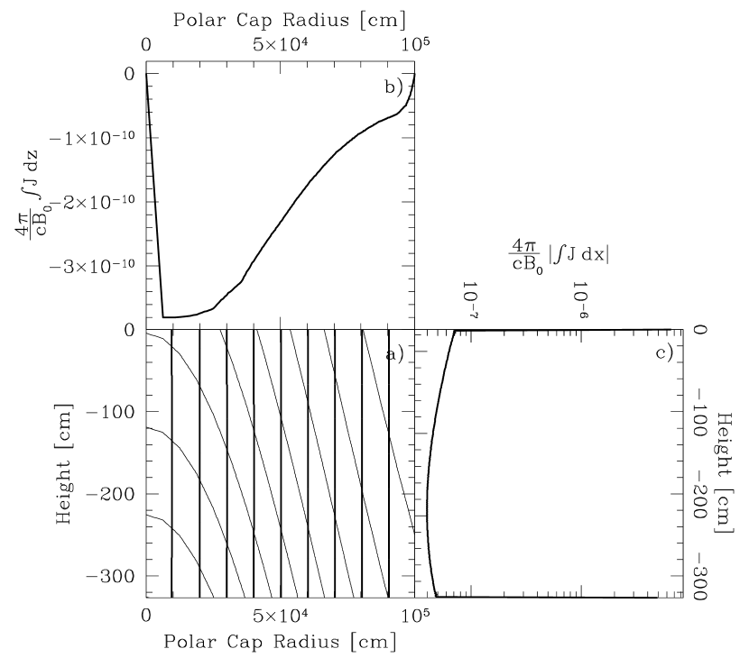
Figure 11: The confinement of accreted matter by a magnetic field. In panel a we show isochores (thin lines) for a matter distribution, at $z\rightarrow\infty$, of $F\propto[1+\exp(-|\varpi/R_{\rm cap}|^{2})]$, where $\varpi$ is the coordinate along the surface. The magnetic field (heavy lines) is assumed to be uniform in the region outside the plot. In panels b and c we show the current density integrated over $z$ and $\varpi$, respectively. The parameter $\beta(H/R_{\rm cap})$ varies from 0.24 at the top to 0.37 at the bottom, so that no appreciable spreading occurs, even though $\beta=8\pi P/B^{2}=74$ at the top ($z=0$). The induced dipole moment (not including the current sheets at the top and bottom) is $\mbox{\boldmath$\displaystyle\mu$}=-0.078B_{0}R_{\rm cap}{}^{3}\mbox{\boldmath$\displaystyle e$}_{z}$.

In Figures 11 and 12 we show two numerical solutions to equation (57). Panel a depicts the constant density contours (thin lines) and the lines of constant flux (thick lines). In panels b and c we show the integral of $J$ over the vertical coordinate $z$ and the radial coordinate $\varpi$, respectively. The matter overpressure induces a dipole moment, opposed to the stellar field, of order $B_{0}R_{\rm cap}{}^{3}$ inside the region. The existence of large current sheets at the top and bottom of the region is evident in panel c. These sheets are required by the boundary conditions that the field be uniform outside the region. In Figure 11 (Fig. 12), the parameter $\beta(H/R_{\rm cap})$ varies from 0.24 (0.97) at the top to 0.37 (6.1) at the bottom. As can be seen in Figure 12a, the maximum displacement of a field line from its equilibrium location is of order $500\,{\rm cm}$, so that $B_{\varpi}/B_{z}$ is of order unity. (The field lines are bent more than is visually apparent from panel a due to the different scales for the vertical and lateral displacements). The induced dipole (not including the current sheets at the top and bottom) is $\mbox{\boldmath$\displaystyle\mu$}=-0.078B_{0}R_{\rm cap}{}^{3}\mbox{\boldmath$\displaystyle e$}_{z}$ ($\mbox{\boldmath$\displaystyle\mu$}=-0.82B_{0}R_{\rm cap}{}^{3}\mbox{\boldmath$\displaystyle e$}_{z}$) for Figure 11 (Fig. 12).

While the field lines threading the crust are anchored in place, the field lines through the outer atmosphere are free to move outward. Because of the large induced dipole, the field lines in the atmosphere will be distorted from the matter-free configuration for a distance $\sim R_{\rm cap}\gg H$ above the ocean.

Figure 12: Same as Fig. 11, except that the matter distribution at $z\rightarrow\infty$ is $F\propto[0.5+\exp(-|\varpi/R_{\rm cap}|^{2})]$, and $\beta(H/R_{\rm cap})$ varies from 0.97 to 6.1. The displacement of the field line from its unperturbed configuration is about $500\,{\rm cm}$, so that $B_{\varpi}/B_{0}$ is of order unity, as expected (note that the vertical and horizontal scales in panel a are greatly different, so that the field line distortion is not as apparent). The induced dipole moment (not including the current sheets at the top and bottom) is $\mbox{\boldmath$\displaystyle\mu$}=-0.82B_{0}R_{\rm cap}{}^{3}\mbox{\boldmath$\displaystyle e$}_{z}$.

References

- [Angelini, Stella, & White 1991] Angelini, L., Stella, L., & White, N. E. 1991, ApJ, 371, 332
- [Arons & Lea 1976] Arons, J. 1976, ApJ, 207, 914
- [Azuma et al. 1994] Azuma, R. E. et al. 1994, Phys. Rev. C, 50, 1194
- [Ayasli & Joss 1982] Ayasli, S., & Joss, P. C. 1982, ApJ, 256, 637
- [Berger & van der Klis 1995] Berger, M., & van der Klis, M. 1995, A&A, 292, 175
- [Bildsten 1995] Bildsten, L. 1995, ApJ, 438, 852
- [Bildsten 1998] Bildsten, L. 1998, in “The Many Faces of Neutron Stars”, ed. A. Alpar, L. Buccheri, & J. van Paradijs, (Dordrecht: Kluwer), in press
- [Bildsten & Brown 1997] Bildsten, L., & Brown, E. F. 1997, ApJ, 477, 897
- [Bildsten & Cumming 1998] Bildsten, L., & Cumming, A. 1998, ApJ, submitted
- [Bildsten & Cutler 1995] Bildsten, L., & Cutler, C. 1995, ApJ, 449, 800
- [Bildsten, Salpeter, & Wasserman 1992] Bildsten, L., Salpeter, E. E., & Wasserman, I. 1992, ApJ, 384, 143
- [Buchmann 1996] Buchmann, L. 1996, ApJ, 468, L127
- [Buchmann 1997] Buchmann, L. 1997, ApJ, 479, L153
- [Caughlan & Fowler 1988] Caughlan, G. R., & Fowler, W. A. 1988, At. Data Nucl. Data Tables, 40, 283
- [Chakrabarty 1998] Chakrabarty, D. 1998, ApJ, 492, 342
- [Chakrabarty et al. 1997] Chakrabarty, D. et al. 1997, ApJ, 474, 414
- [Champagne & Wiescher 1992] Champagne, A. E., & Wiescher, M. 1992, Annu. Rev. Nucl. Part. Sci., 42, 39
- [Cox & Giuli 1968] Cox, J. P., & Giuli, R. T. 1968, Principles of Stellar Structure, Vol. 1 (New York: Gordon and Breach)
- [Dal Fiume et al. 1997] Dal Fiume, D., et al. 1997, IAU Circ., 6608
- [Elsner & Lamb 1977] Elsner, R. F., & Lamb, F. K. 1977, ApJ, 215, 897
- [Farouki & Hamaguchi 1993] Farouki, R. T., & Hamaguchi, S. 1993, Phys. Rev. E, 47, 4330
- [Freidberg 1987] Freidberg, J. P. 1987, Ideal Magnetohydrodynamics (New York: Plenum)
- [Fujimoto et al. 1984] Fujimoto, M. Y., Hanawa, T., Iben, I., Jr., Richardson, M. B. 1984, ApJ, 278, 813
- [Fujimoto et al. 1981] Fujimoto, M. Y., Hanawa, T., & Miyaji, S. 1981, ApJ, 247, 267
- [Fushiki 1986] Fushiki, I. 1986, PhD thesis, Harvard Univ.
- [Fushiki & Lamb 1987a] Fushiki, I., & Lamb, D. Q. 1987a, ApJ, 317, 368
- [Fushiki & Lamb 1987b] Fushiki, I., & Lamb, D. Q. 1987b, ApJ, 323, L55
- [Geppert & Urpin 1994] Geppert, U., & Urpin, V. 1994, MNRAS, 271, 490
- [Ghosh & Lamb 1979] Ghosh, P., & Lamb, F. K. 1979, ApJ, 234, 296
- [Haensel & Zdunik 1990] Haensel, P., & Zdunik, J. L. 1990, A&A, 227, 431
- [Hameury et al. 1983] Hameury, J. M., Bonazzola, S., Heyvaerts, J., & Lasota, J. P. 1983, A&A, 128, 369
- [Hansen 1973] Hansen, J.-P. 1973, Phys. Rev. A, 8, 3096
- [Homer et al. 1996] Homer, L., Charles, P. A., Naylor, T., van Paradijs, J., Auriere, M., & Koch-Miramond, L. 1996, MNRAS, 282, L37
- [Joss & Li 1980] Joss, P. C., & Li, F. K. 1980, ApJ, 238, 287
- [Konar & Bhattacharya 1997] Konar, S., & Bhattacharya, D. 1997, MNRAS, 284, 311
- [Lamb & Lamb 1978] Lamb, D. Q., & Lamb, F. K. 1978, ApJ, 220, 291
- [Lamb et al. 1973] Lamb, F. K., Pethick, C. J., & Pines, D. 1973, ApJ, 184, 271
- [Landau & Lifshitz 1980] Landau, L. D., & Lifshitz, E. M. 1980, Statistical Physics (3d ed.; Tarrytown: Pergamon)
- [Levine et al. 1991] Levine, A., Rappaport, S., Putney, A., Corbet, R., Nagase, F. 1991, ApJ, 381, 101
- [McClintock et al. 1977] McClintock, J. E., Rappaport, S. A., Nugent, J. J., and Li, F. K. 1977, ApJ, 216, L15
- [Miralda-Escudé et al. 1990] Miralda-Escudé, J., Haensel, P., & Paczyński, B. 1990, ApJ, 362, 572
- [Nelson et al. 1986] Nelson, L. A., Rappaport, S., & Joss, P. C. 1986, ApJ, 304, 231
- [Paczyński 1983] Paczyński, B. 1983, ApJ, 267, 315
- [Parmer et al. 1989] Parmer, A. N., White, N. E., Stella, L., Izzo, C., & Ferri, P. 1989, ApJ, 338, 359
- [Pethick & Sahrling 1995] Pethick, C. J., & Sahrling, M. 1995, ApJ, 453, L29
- [Ogata, Ichimaru, & Van Horn 1993] Ogata, S., Ichimaru, S., & Van Horn, H. M. 1993, ApJ, 417, 265
- [Romani 1990] Romani, R. W. 1990, Nature, 347, 741
- [Salpeter & Van Horn 1969] Salpeter, E. E., & Van Horn, H. M. 1969, ApJ, 155, 183
- [Schatz et al. 1998] Schatz, H. et al, 1998, Phys. Rep., 294, 167
- [Schmalbrock et al. 1983] Schmalbrock, P., et al. 1983, Nucl. Phys. A, 398, 279
- [Schinder et al. 1987] Schinder, P. J., Schramm, D. N., Wiita, P. J., Margolis, S. H., & Tubbs, D. L. 1987, ApJ, 313, 531
- [Shibazaki & Lamb 1989] Shibazaki, N., & Lamb, F. K. 1989, ApJ, 346, 808
- [Smit & van der Klis 1996] Smit, J. M., & van der Klis, M. 1996, A&A, 316, 115
- [Spitzer 1962] Spitzer, L. Jr. 1962, Physics of Fully Ionized Gases (2d ed.; New York: Wiley)
- [Taam 1982] Taam, R. E. 1982, ApJ, 258, 761
- [Taam 1985] Taam, R. E. 1985, Annu. Rev. Nucl. Part. Sci., 35, 1
- [Taam & Picklum 1978] Taam, R. E., & Picklum, R. E. 1978, ApJ, 224, 210
- [Taam & Picklum 1979] Taam, R. E., & Picklum, R. E. 1979, ApJ, 233, 327
- [Taam et al. 1996] Taam, R. E., Woosley, S. E., & Lamb, D. Q. 1996, ApJ, 459, 271
- [Timmes 1992] Timmes, F. X. 1992, ApJ, 390, L107
- [Timmes & Woosley 1992] Timmes, F. X., & Woosley, S. E. 1992, ApJ, 396, 649
- [Urpin & Geppert 1995] Urpin, V., & Geppert, U. 1995, MNRAS, 275, 1117
- [Urpin & Geppert 1996] Urpin, V., & Geppert, U. 1996, MNRAS, 278, 471
- [Urpin & Yakovlev 1980] Urpin, V. A., & Yakovlev, D. G. 1980, AZh, 57, 738
- [van Kerkwijk 1993] van Kerkwijk, M. H. 1993, A&A, 276, L9
- [van Kerkwijk et al. 1996] van Kerkwijk, M. H., Geballe, T. R., King, D. L., van der Klis, M., & van Paradijs, J. 1996, A&A, 314, 521
- [van Kerkwijk et al. 1992] van Kerkwijk, M. H., et al. 1992, Nature, 355, 703
- [Van Wormer et al. 1994] Van Wormer, L., Görres, J., Iliadis, C., Wiescher, M., & Thielemann, F.-K. 1994, ApJ, 432, 326
- [Wallace & Woosley 1981] Wallace, R. K., & Woosley, S. E. 1981, ApJS, 45, 389
- [Weaver & Woosley 1993] Weaver, T. A., & Woosley, S. E. 1993, Phys. Rep., 227, 65
- [Woosley & Taam 1976] Woosley, S. E., & Taam, R. E. 1976, Nature, 263, 101
- [Yakovlev & Urpin 1980] Yakovlev, D. G., & Urpin, V. A. 1980, AZh, 57, 526