Outflow collimation in young stellar objects

Abstract

In this paper we explore the effect of radiative losses on purely hydrodynamic jet collimation models applicable to Young Stellar Objects (YSOs). In our models aspherical bubbles form from the interaction of a central YSO wind with an aspherical circum-protostellar density distribution. Building on a previous non-radiative study (Frank & Mellema 1996) we demonstrate that supersonic jets are a natural and robust consequence of aspherical wind-blown bubble evolution. The simulations show that the addition of radiative cooling makes the hydrodynamic collimation mechanisms studied by Frank & Mellema (1996) more effective. We find a number of time-dependent processes contributing to the collimation whose relative strength depends on the age of the system and parameters characterising the wind and the environment. As predicted by Frank & Mellema (1996) the flow-focusing at an oblique inner shock becomes more effective when radiative cooling is included. An unexpected result of this is the production of cool ($T<10^{4}$ K), dense ($n\approx 10^{4}$ cm^-3) jets forming through conical converging flows at the poles of the bubbles. For steady winds the formation of these jets occurs early in the bubble evolution. At later times we find that the dynamical and cooling time scales for the jet material become similar and the jet beam increases in temperature ($T\approx 10^{6}$ K). The duration of the cool jet phase depends on the mass loss rate, $\dot{M}_{\rm w}$, and velocity, $V_{\rm w}$, of the wind. High values of $\dot{M}_{\rm w}$ and low values of $V_{\rm w}$ produce longer cool jet phases.

Since observations of YSO jets show considerable variability in the jet beam we present a simple one-dimensional (1-D) model for the evolution of a variable wind interacting with an accreting environment. We find that the accretion ram pressure can halt the expansion of the bubble on time scales comparable to the periodicity of the wind and length scales less than 100 AU, the approximate observed scale for YSO jet collimation. These models indicate that, in the presence of a varying protostellar wind, the hydrodynamic collimation processes studied in our simulations can produce cool jets with sizes and time scales consistent with observations.

1 Introduction

A large fraction of stars begin their lives in the midst of narrow supersonic streams of gas or ‘jets’. These jets are a common phenomenon and are observed to carry away large amounts of energy and momentum from the central regions of Young Stellar Objects (YSOs). The propagation of these jets has been well studied both analytically [Raga & Kofman 1992] and with sophisticated numerical tools [Blondin, Fryxell & Königl 1990, Stone & Norman 1994a]. However, the processes responsible for collimation remains an unsolved problem. The current consensus favours collimation through magnetohydrodynamical (MHD) effects [Königl 1989, Pudritz 1991, Shu et al. 1994]. While these models are promising they may require conditions which are not achieved in real YSO environments (such as particular field geometries and long collimation scale lengths). In addition some numerical simulations based on these MHD models show that while winds can effectively be produced collimation into a steady jet may be more difficult to achieve [Romanova et al. 1996]. Hydrodynamic collimation models such as DeLaval nozzles [Königl 1982, Raga & Cantó 1989] have fallen out of favour because of length scale requirements [Königl & Ruden 1993], stability considerations [Koo & McKee 1992], and the lack of an energy source to drive the outflow. Especially for low mass stars one can show that the outflows cannot be generated by radiation pressure. However, if one separates the issues of wind acceleration and jet collimation this last point is not a real objection. One can then have initial acceleration through an MHD process and collimation through a hydrodynamic process. In weighing the relative advantages of hydrodynamic and MHD collimation models it is clear that the hydrodynamic models offer the advantage of being simpler in terms of underlying physical processes and requirements on initial conditions.

Until recently the majority of jet collimation models, both hydrodynamic and MHD, have been analytic. To reduce the complexity of the equations involved, these models need simplifying assumptions which typically involve ignoring the time-dependence in the equations, in other words steady state solutions. This impliesignoring the dynamical feedback of the global flow [Raga & Cantó 1989] and freezing initial configurations such as exterior pressure distributions. These assumptions, though necessary to make initial progress, are suspect from first principles. In addition, it has become clear that the flows in YSO jets are essentially unsteady. Recent observations of HH jets show strong evidence for velocity variations within the jet beam [Hartigan et al. 1992], [Hartigan et al. 1996]. Molecular outflows, which may be driven by jets [Chernin et al. 1994], also show evidence for episodic variations in outflow speed and density [Bachiller, Tafalla, & Cernichado 1994]. These observations suggest that the driving of the YSO outflow and its interaction with the circumstellar environment are fundamentally time-dependent processes, and time-dependent numerical models are needed.

In a recent work Frank & Mellema [Frank & Mellema 1996] (hereafter FM96) revisited the issue of purely hydrodynamic collimation mechanism using high resolution numerical simulations. FM96 focused on the interaction of a wind from a protostar wind with an aspherical (toroidal) circum-protostellar environment. Studies of planetary nebulae have demonstrated that this kind of interaction can produce well collimated jets [Icke et al. 1992]. The mechanism has been called “Shock-Focused Inertial Confinement” (SFIC). In the SFIC mechanism it is the inertia of a toroidal environment rather than its thermal pressure, which produces a bipolar wind-blown bubble. The bubble’s reverse shock, which decelerates the wind, takes on an aspherical, prolate geometry [Eichler 1982]. The radially streaming central wind strikes this prolate shock obliquely focusing it towards the polar axis and initiating the jet collimation. Other effects such as instabilities along the walls of the bubble, help to maintain the collimation of the shocked wind flow.

In an initial study Frank & Noriega-Crespo [Frank & Noriega-Crespo 1994] used non-radiative numerical simulations to demonstrate that the SFIC mechanism can produce jets in the context of YSOs. Peter & Eichler [Peter & Eichler 1995] studied the inertial confinement of fully formed jets in a more general context. FM96 carried out a more extensive study of the SFIC mechanism in YSO systems. The high resolution simulations presented in FM96 showed that a central wind interacting with a toroidal shaped density distribution naturally leads to the development of strongly collimated supersonic flows. Toroidal density distributions are theoretically expected to form from the collapse of a rotating cloud [Tereby, Shu & Cassen 1984] or of a flattened filament [Hartmann, Calvet, & Boss 1996], or of a magnetised cloud [Li & Shu 1996]. In addition there is also some observational evidence for such structures [Lucas & Roche 1997, Kraemer et al. 1997].

The collimated supersonic flows found in the simulations are accompanied by all the usual features expected for gaseous jets: bow and jet shocks; turbulent cocoons; crossing shocks and internal Mach disks. Because the aim of FM96 was to explore the basic physics of the SFIC mechanism in detail they used simulations without cooling and then applied analytical models to explicate the underlying dynamics. In this way FM96 showed the dual nature of the collimated flow as both a supersonic jet and a wind-blown bubble. More importantly they also concluded that even a small degree of asphericity in the reverse shock is sufficient to produce strong flow focusing (cf. Icke 1988). Using an analytical approximation to estimate the effects of radiative cooling they found that with radiative cooling included these shocks are capable of achieving collimation on length scales smaller than 100 AU, consistent with the HST observations [Heathcote et al. 1996, Burrows et al. 1996]. Their analytical models also showed that flow focusing becomes even more effective in cooling shocks (cf. Icke 1988). This allows the wind to be redirected into a jet without becoming subsonic.

While the results of FM96 were promising many questions remain to be answered. These include: the dynamical role of cooling; the effect of more realistic environments; the connection with YSO observables. Each of these issues deserves considerable attention. Our philosophy in pursuing this line of research is to isolate domains of interest and use simulations as numerical experiments to reveal and then articulate the underlying physical processes. Following this strategy we focus here on the first question: the dynamical effect of radiative cooling. As we will demonstrate the addition of cooling to the simulations produces dramatic changes in the flow which enhance the previously studied non-radiative SFIC collimation process, as was predicted in FM96. What was not predicted is a new collimation process, which operates when radiative cooling is included. This process, first explored in a series of papers by Tenorio-Tagle, Cantó & Różyczka [Tenorio-Tagle, Cantó & Różyczka 1988], may be applicable to jet collimation not only in YSOs but also in other objects, such as planetary nebulae [Frank, Balick & Livio 1996, Mellema 1996]. Some of the results seen in our simulations are found in a more general and more abstracted series of simulations done by Peter & Eichler [Peter & Eichler 1996]. Their results confirm the efficacy of the radiative collimation processes explored in a more dynamical context here.

The organization of the paper is as follows: In Section 2 we describe the numerical method and initial conditions used in our simulations. In Section 3 we present and discuss the results of our simulations. In Section 4 we address the wind variability. Finally in Section 5 we present our conclusions along with a discussion of some issues raised by the simulations.

2 Computational Methods and Initial Conditions

The hydrodynamic interactions we wish to study are governed by the Euler equations with a ‘sink’ term due in the energy equation due to radiative losses.

$${\partial\rho\over\partial t}+\mn@boldsymbol{\nabla}\cdot\rho\mn@boldsymbol{u}=0\,,$$ (1)

$${\partial\rho\mn@boldsymbol{u}\over\partial t}+\mn@boldsymbol{\nabla}\cdot\rho\mn@boldsymbol{uu}=\mn@boldsymbol{\nabla}P\,,$$ (2)

$${\partial E\over\partial t}+\mn@boldsymbol{\nabla}\cdot\mn@boldsymbol{u}(E+p)=-{x^{2}_{\rm i}\rho\over\bar{m}}^{2}\Lambda(T)-{\partial x_{\rm i}\over\partial t}I_{\rm H}\,,$$ (3)

where

$$E={1\over 2}\rho|\mn@boldsymbol{u}|^{2}+{p\over(\gamma-1)}\,,$$ (4)

and

$$p={\rho kT\over\bar{m}}\,.$$ (5)

In the above equations ${\bar{m}}$ is the mean mass per particle, $x_{\rm i}$ is the fraction of ionized hydrogen, and we take $\gamma=5/3$.

2.1 Numerical methods

We have carried out our study using two different numerical codes each of which is cast in a different coordinate geometry. All the simulations are run in two dimensions, assuming cylindrical symmetry. The first code is based on a Roe-solver method [Mellema, Eulderink & Icke 1991] and uses spherical coordinates ($R,\theta$). The second code is based on the Total Variation Diminishing (TVD) method of Harten [Harten 1983] as implemented by Rye et al. [Ryu et al. 1995]. The TVD code solves the Euler equations in cylindrical coordinates ($r,z$). Both codes are explicit methods for solving hyperbolic systems of equations. Second order accuracy is achieved by finding approximate solutions to the Riemann problem at grid boundaries. Oscillations are prevented by using a lower order monotone scheme near steep changes.

Previous experience [Frank & Mellema 1994] has shown us the value of using two different codes, based on different numerical methods and applied with different geometries, to work on the same problem. One of the most difficult aspects of numerical studies is knowing to which extend one can trust the results. Applying two codes to the same problem can quickly and convincingly root out numerical artifacts. We note that the TVD code in its present configuration is more diffusive than the Roe solver code and this fact must be considered in comparing their results in detail. The main point we wish to make in comparing the two codes is that both produce hydrodynamically collimated jets via the same mechanisms.

In both codes cooling is included using operator splitting and is calculated from look-up tables for $\Lambda(T)$ taken from the coronal cooling curve of Dalgarno & McCray [Dalgarno & McCray 1972]. The treatment of the cooling term is different in both codes. For the Roe solver the collisional ionization equation for hydrogen is solved first and the computed value of $x_{\rm i}$ is fed into equation 3. The cooling source term is then integrated into the solution through iteration. Cooling through collisional ionization of hydrogen (the ${\partial x_{\rm i}\over\partial t}I_{\rm H}$ term) is also taken into account. Because of the iteration it is not necessary to set a cooling time limit on the time step, although in practise it helps to avoid numerical problems.

In the TVD code full ionization is assumed and the cooling is applied via an integration of the thermal energy ($E_{\rm t}$) equation

$${dE_{\rm t}\over dt}=-{\dot{E}_{\rm t}}=\left({\rho\over\bar{m}}\right)^{2}\Lambda(T)\,.$$ (6)

For application to the simulations the solution to this equation takes the form

$${E_{\rm t}}^{n+1}={E_{\rm t}}^{n}\exp(-{{\dot{E}_{\rm t}}\over{E_{\rm t}}^{n}}\Delta t)\,,$$ (7)

where the superscript $n$ refers to the time index ($t^{n}=n\Delta t$). The term in the exponential can be expressed as as $\Delta t/\Delta t_{\rm c}$ where $\Delta t_{\rm c}$ is the local cooling time scale of the gas: $\Delta t_{\rm c}={\dot{E}_{\rm t}}/E_{\rm t}$. This formulation has the advantage protecting ${E_{\rm t}}^{n+1}$ from becoming negative in regions of strong cooling. In practice one must choose the time step $\Delta t$ so as not to be in conflict with short cooling time scales. We use

$$\Delta t=\min[\Delta t_{\rm hydro},1.5\Delta t_{\rm c}]\,,$$ (8)

where $\Delta t_{\rm hydro}$ is the hydrodynamic time step set by the Courant condition.

Both codes have been tested against analytical models of wind-blown bubbles [Koo & McKee 1992] and were found to recover appropriate values of various shock positions and velocities.

2.2 Initial conditions

The initial conditions used in our simulations are identical to those used in FM96 and we refer the reader to that paper for the details. Our simulations begin with a stationary isothermal environment characterized by a aspherical (toroidal) density distribution. We have used a distribution $\rho(r,\theta)$ which creates a pseudo-disk of FWHM $=90^{\circ}$. The input parameters for the environment are the mass of the central protostellar object (taken to be $M=1$M_⊙), the accretion rate ${\dot{M}_{\rm a}}$ which determines the density in the environment, and finally, the equator to pole density contrast $q=\rho(0^{\circ})/\rho(90^{\circ})$. In the FM96 it was found that supersonic jets were produced for $q>7$.

As in FM96 we do not include infall velocity, nor the effects of gravity or rotation. As was noted in the introduction the aim is to isolate the effects of radiative cooling on the collimation models. In Section 4 we present analytical models that will address the effects of both gravity and accretion ram pressure on the the bubble dynamics and jet collimation. In addition the next paper in this series will focus on the SFIC collimation in more realistic environments [cf. Yorke, Bodenheimer & Laughlin 1993, Hartmann, Calvet, & Boss 1996].

An even further complication would be a non-axisymmetric accreting environment. How such an environment affects the flow cannot be addressed without 3-D models which is beyond the scope of the present work. One may also worry about the longevity of the toroidal density distributions. However, both Li & Shu [Li & Shu 1996] and Matsumoto, Hanawa & Nakamura [Matsumoto, Hanawa & Nakamura 1997] find self-similar (i.e. scale free) toroidal structures in their models, implying that the accretion flow will maintain this geometry over a long time span.

The central protostellar wind is fixed in an inner sphere of grid cells. The relevant input parameters are simply the mass loss rate ${\dot{M}_{\rm w}}$ and velocity $V_{\rm w}$ in the wind.

In Table 1 we list the relevant input parameters for the 5 simulations presented in this paper. We have carried out more than 30 simulations including a sequence of simulations at different resolutions ($64\times 320$; $128\times 640$; $256\times 1280$). These convergence tests demonstrate that the main collimation features are adequately resolved (though we have not reached full convergence). A comparison between the $128\times 640$ and $256\times 1280$ results shows that the higher resolution simulations reveal more detail but do not show changes in overall flow pattern.

However, our flow solutions do contain strong cooling regions which often our grids cannot adequately resolve. One must therefore be careful in interpreting the results as under-resolved cooling zones may lead to grid mixing. Problems like these can only be addressed by continued modelling at higher resolution when additional computational resources become available. However, seeing similar flow patterns in two different codes configured in different geometries strengthens the argument that we are seeing real physical effects rather than numerical artifacts. In fact very similar results have also been found when using a PPM (Piecewise Parabolic Method) code using an expanding grid to study strongly cooling wind-blown bubbles in the context of planetary nebulae (Dwarkadas, private communication). Thus the development of hydrodynamically collimated jets in wind-blown bubbles has been found in two different sets of numerical experiments with three different kinds of numerical tools.

Table 1: Initial Conditions For Runs A – E

run	${\dot{M}}_{\rm w}$	$V_{\rm w}$	${\dot{M}}_{\rm a}$	$q$	resolution
A	$1\times 10^{-7}$	350	$1\times 10^{-6}$	70	$256\times 1536$
B	$2\times 10^{-7}$	250	$1\times 10^{-5}$	70	$256\times 1280$
C	$1\times 10^{-7}$	450	$5\times 10^{-6}$	60	$256\times 1280$
D	$1\times 10^{-6}$	250	$1\times 10^{-7}$	50	$250\times 250$
E	$1\times 10^{-8}$	250	$1\times 10^{-9}$	50	$250\times 250$

3 Simulation Results

Here we present the results of several numerical simulations, calculated with both methods introduced above (TVD and Roe solver). We explore two sequences in parameter space, runs A to C form a sequence in outflow velocity (from 250 to 450 km $\rm{s}^{-1}$), calculated with the TVD-method. Runs D and E (calculated with the Roe solver) form a sequence in density, which serves to illustrate the importance of cooling. See Table 1. We mainly concentrate on describing the results of run A, and then point out some of the differences with the other runs.

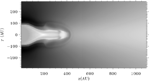
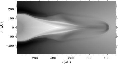
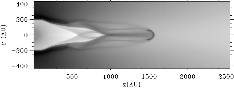
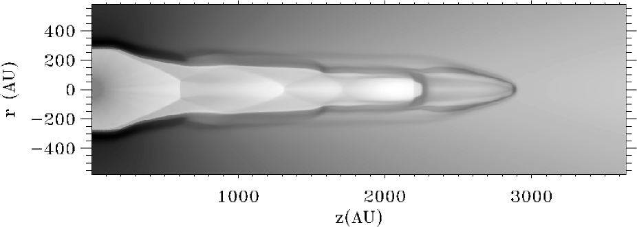
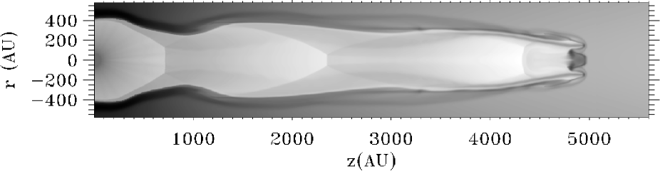
Figure 1: Density evolution for run A. The grey scales show $\log_{\rm 10}$ contours for times $t=$25, 62, 87, 137, 225 years. The darker shades are higher density. One sees the initial radiative phase, the development of the ‘cool jet’ and the development of the ‘hot jet’. The minimum/maximum pairs in units of cm^-3 are $(152,4.95\times 10^{6})$, $(80.2,4.05\times 10^{6})$, $(76.3,3.78\times 10^{6})$, $(24.8,3.20\times 10^{6})$, $(4.38,1.976\times 10^{6})$. See also Fig. 2.

3.1 Cool jet

The evolution of the flow pattern in run A is shown in Figs. 1 and 2. They show the density and temperature in logarithmic grey scales. One sees how initially the interaction creates an aspherical bubble, which is almost completely radiative. The freely expanding wind extends almost all the way to the shell of swept up ambient material. In the temperature plot (Fig. 2) one can see the thin cooling layer separating the outflow and the swept-up material and a small reservoir of hot gas at the very tip of the bubble.

As time progresses, a unique feature forms at the top of the bubble (Figs. 1b and 2b). This structure takes the form of a dense, high velocity jet, with a relatively low temperature, ($T\approx 10^{4}$ K), which is still higher than that of the surroundings. By tracking the advection of a passive fluid tracer we are able to identify the location of wind and ambient fluids at all times. This shows that the jet is composed only of wind material. The formation of this ‘cool jet’ is seen in all the TVD-code and the Roe-solver simulations where the cooling time scales are short. In addition the ‘cool’ jet formation occurs for a large range of outflow velocities as we will show below. The collimation process we see in our simulations appears to be related to the jet formation mechanism originally suggested by Cantó & Rodríguez [Cantó & Rodriguez 1980] and later studied by Cantó, Tenorio-Tagle & Różyczka [Cantó, Tenorio-Tagle & Różyczka 1988] (hereafter: CTTR) and Tenorio-Tagle et al. [Tenorio-Tagle, Cantó & Różyczka 1988] (hereafter: TTCR) using idealized analytical and numerical models. In the models of Cantó and collaborators a jet is formed by flows converging at the top of a radiative wind-driven bubble. A shock forms at the apex of the converging flow which redirects material into a narrow beam. We note that in the studies of CTTR and TTCR the converging beams were imposed as initial conditions. In our results they are a natural and robust consequence of the interaction between the outflow and the surrounding material.

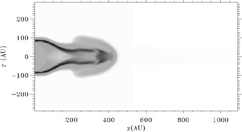
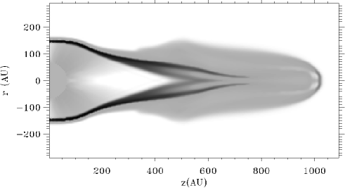
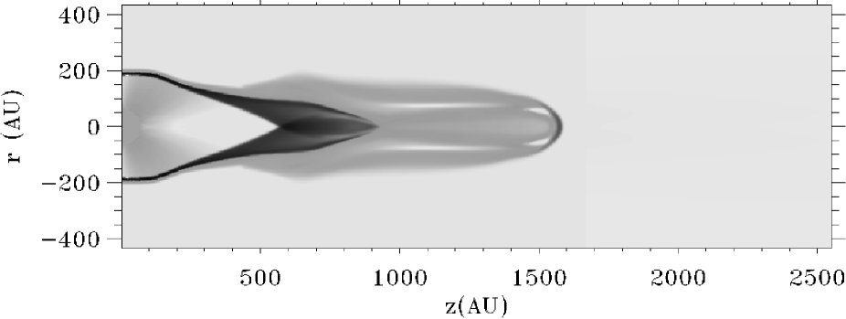
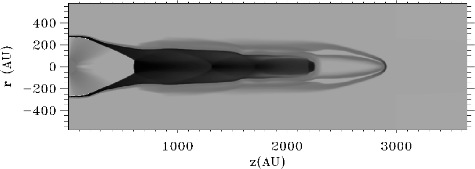
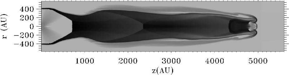
Figure 2: Temperature evolution for run A. The grey scales show $\log_{\rm 10}$ contours for times $t=$25, 62, 87, 137, 225 years. The darker shades are higher temperatures. Note the presence of high temperature gas filling much of the volume in the first frame. The minimum/maximum pairs in units of K are $(993,1.98\times 10^{6})$, $(988,1.86\times 10^{6})$, $(429,2.76\times 10^{6})$, $(12.4,2.97\times 10^{6})$, $(28.6,3.12\times 10^{6})$.

The angle of incidence (between the beam and the symmetry axis) is quite low here. This can be seen in Fig. 3, which shows a contour plot of the direction of the flow at the base of the jet ($t=62$ years). The quantity plotted is the direction of the flow vectors, the contours running from $-6^{\circ}$ to $0^{\circ}$, and negative angles implying a direction towards the symmetry axis. One can see how there is a beam flowing towards the axis at an angle of about $-5^{\circ}$, and how a jet (with flow angle close to $0^{\circ}$) forms at the axis. An angle of incidence of $5^{\circ}$ is lower than any of the cases explored by TTCR But low angles are actually a good condition for the mechanism, since not much kinetic energy is lost in the shock. In fact the shock is so weak here that it is hardly noticeable. At the same time the collimation is very effective, something that could already be seen in the results of CTTR and TTCR.

Although the same idea lies behind the work of CTTR and TTCR and the results presented here, there are some important differences. In CTTR the bubble was assumed to be in pressure equilibrium with the surroundings, which is not the case here. This has implications for the long term evolution of these structures, something we will come back to in Section 4. Both the analytical models of CTTR and the numerical models of TTCR were further simplified by assuming a steady state configuration at the base of the flow with completely homogeneous beams colliding at the symmetry axis. Our flow is time-dependent and far from homogeneous. The converging flows which appear in our simulations have density, velocity and pressure varying with position. The idealization we do have in common with the previous work is the assumption of a perfect, ‘rigid’ symmetry axis.

Figure 3: Contour plot of the angle of flow for run A. Only the area with the converging flow is shown. The symmetry axis is on the left. Contours are $-6^{\circ}$, $-5^{\circ}$, $-4^{\circ}$, $-3^{\circ}$, $-2^{\circ}$, $-1^{\circ}$, $0^{\circ}$. An angle of $0^{\circ}$ means flow parallel to the symmetry axis and negative values mean flow pointing towards the symmetry axis.

Despite these differences it is still instructive to make a simple comparison between the analytic models and the behaviour in the simulations. The input parameters for the CTTR model are the initial density $\rho_{0}$, width $y_{0}$, and angle of incidence $\theta$ of the converging flow as well as the inverse compression ratio $\zeta$ across shock at the tip of flow ($\zeta=1/4$ for a non-radiative shock). CTTR derived the following equations for the jet radius $r_{\rm j}$, length $d_{\rm j}$, density $\rho_{\rm j}$, and velocity $v_{\rm j}$:

$$r_{\rm j}={y_{0}\tan{\alpha}\over\tan\alpha+\tan\theta}\,,$$ (9)

$$d_{\rm j}={y_{0}\over\tan\alpha+\tan\theta}\,,$$ (10)

$$\rho_{\rm j}=\rho_{0}{1+\tan\theta/\tan\alpha\over\zeta}\,,$$ (11)

$$v_{\rm j}=v_{0}\cos(\theta+\alpha)/\cos\alpha\,,$$ (12)

where $\alpha$ is the half opening angle of the shock at the tip of the converging flow or in other words the angle between the shock and the symmetry axis,

$$\tan\alpha={(1-\zeta)-\sqrt{(1-\zeta)^{2}-4\zeta\tan^{2}\theta}\over 2\tan\theta}\,.$$ (13)

Taking values from the situation shown in Fig. 3 we have an angle of incidence $\theta$ of around $5^{\circ}$ and a beam velocity $v_{0}$ of approximately 300 km $\rm{s}^{-1}$. For a qualitative comparison we assume the adiabatic case (i.e. using an inverse compression factor of $\zeta=0.25$ since the shocks are weak) which leads to a jet opening angle $\alpha$ of $1\aas@@fstack{\circ}7$, or nearly perfect collimation. The width of the beam $y_{0}$ at the convergence point ($z=540$ AU) is measured to be approximately 12 cell sizes (or $6.5\times 10^{14}$ cm), leading to a jet cross section $r_{\rm j}$ of 3 cell sizes (or $1.6\times 10^{14}$ cm) and a length $d_{\rm j}$ of 102 cell sizes (or $5.6\times 10^{15}$ cm), both approximately consistent with the result in the simulation. For the derived values of $\theta$ and $\alpha$ the jet velocity $v_{\rm j}$ turns out to be 0.99 of the beam velocity, so $\sim 300$ km s^-1, and the shock velocity $v_{\rm s}^{0}$ a factor 0.12 of that, so around 36 km s^-1, making it approximately a (weak) Mach 2 shock. The density of the beam is far from homogeneous, ranging from 1000 to 5000 cm^-3 which, still following the CTTR model, would lead to jet densities of 16,000 to 80,000 cm^-3. In our simulation the jet density varies from 20,000 to 50,000 cm^-3. So, within all the uncertainties the match between the analytic description and the simulation is quite good, showing that it is indeed the convergence of conical flows that produces the initial jet in these simulations.

Following the evolution of this ‘cool jet’ we find that the bow shock of the jet has a velocity of $\approx$ 110 km $\rm{s}^{-1}$. The flow velocity in the jet beam lies between 160 and 200 km $\rm{s}^{-1}$ and typical values for the Mach number are around 16 (at $t=62$ years), and 35 (at $t=112$ years), so the jet is highly supersonic. The temperature in the main body of the jet is around 1,000 K (but several 100,000 at the head), and the density is typically 2,000 $\rm{cm}^{-3}$, at $t=112$ years (though ten times as large in the earlier phases, $t\sim 60$ years). The width of the main channel is about 100 AU (five to ten times the width of the initial focusing region), the wings adding another 50 AU.

As we said in Section 2, resolution effects may affect the details of the numerical results. The presence of density gradients in the focusing region may be real or may be due to grid-mixing. The same is true for the role of instabilities (particularly Kelvin-Helmholtz) which may not be captured in these simulations. Future studies will need to address these points using higher resolution studies.

3.2 Hot jet

The further evolution of the jet is influenced by another change in the structure of the flow pattern. At about $t=80$ years a high temperature ($T\sim 10^{6}$ K) region develops at the top of the bubble and the base of the jet (Figs. 1c and 2c). The emergence of this high temperature gas marks the transition from a radiative to an adiabatic configuration. This transition starts at the poles because the densities are lowest there, and consequently the cooling time longer. The transition from radiative to adiabatic can be followed by looking at the shape of the wind shock. At $t=62$ years it is very aspherical with an an ellipticity of $e=0.33$ where $e=R_{\rm sw}(0^{\circ})/R_{\rm sw}(90^{\circ})$ and $R_{\rm sw}$ is the radius of the wind shock. As time progresses the shape relaxes. At $t=225$ years the wind shock has reached an ellipticity of only $e=0.5$. We note however that FM96 found some degree of asphericity even in the fully non-radiative case and that this was sufficient to produce collimation.

The high pressure region at the top of the bubble develops its own jet structure in much the same way as was described in FM96. Although the gas is decelerated at the wind shock, the constriction in the flow channel (the contact discontinuity) quickly re-accelerates the flow so that it almost reaches the original wind velocity (350 km $\rm{s}^{-1}$). A DeLaval nozzle is not needed however. The obliqueness of the shock relative to the free streaming wind at lower latitudes is high enough that post-shock material is focused towards the axis but never becomes subsonic. This focusing effect for aspherical wind shocks was described in FM96 where we predicted that the collimated flow behind the oblique shock could retain its supersonic character. The calculations presented in that paper also demonstrated that this effect becomes stronger when some degree of post-shock cooling is included. This is exactly what is observed in the simulations presented here. This also shows that the inclusion of cooling does not invalidate the results obtained for the non-cooling case. In fact, as was argued in FM96, cooling enhances some of hydrodynamic collimation effects, such as the asphericity of the wind shock.

This second jet, or ‘hot jet’, has a Mach number at the base of about 3 to 4. It catches up with the slower ‘cool jet’ and in the last frame has almost completely overtaken it ($t=225$ years). In the mean time it develops similarly to the hot jets described in Paper I, forming internal working surfaces. These working surfaces are not stationary, but travel along the jet with pattern velocities of around 50 to 100 km $\rm{s}^{-1}$, not unlike the observed ones. As the jet grows, material in its beam continues to cool and the temperature drops from about $2\times 10^{6}$ K just after an internal working surface to about $2\times 10^{5}$ K just before the next one. Since the velocity does not change the Mach number of the jet grows as material traverses the beam reaching values as high as $M\approx 8$ just before an internal working surface. A vector plot of the velocity field at $t=225$ years is shown in Fig. 4.

Figure 4: The velocity field for run A at $t=225$ years. The length of the vectors is proportional to the absolute value of the velocity. The maximum value is 350 km $\rm{s}^{-1}$ and the minimum 0 km $\rm{s}^{-1}$. One can see the focusing at the base of the jet and near the internal working surface.

Thus, our simulation shows a sequence of two jets, an early ‘cool jet’ formed by the focusing of the outflow along the inner shock of a momentum-driven bubble, and a later ‘hot jet’ formed by the SFIC mechanism described in FM96. As the system evolves this second jet overtakes the first.

3.3 Different wind velocities

Run B has almost the same parameters as run A except for a mass loss rate thats higher by a factor of 2 and a wind velocity which is 250 km $\rm{s}^{-1}$. Because of this lower wind speed one expects cooling to play a more important role ($T_{\rm shock}\propto V_{\rm shock}^{2}$) and we do find that in this case the cool jet phase persists for a far longer time (about a factor of 5). We note however that the same sequence of cool to hot jet that was seen in run A also occurs in B and the results of runs A and B look similar when they have reached similar size scales. Run C with a 450 km $\rm{s}^{-1}$ outflow also develops both a cool and a hot jet phase but here the cool jet phase lasts only for a short time. Fig. 5 shows the comparison of the jets for runs B and C.

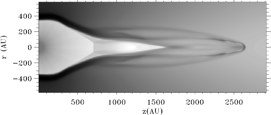
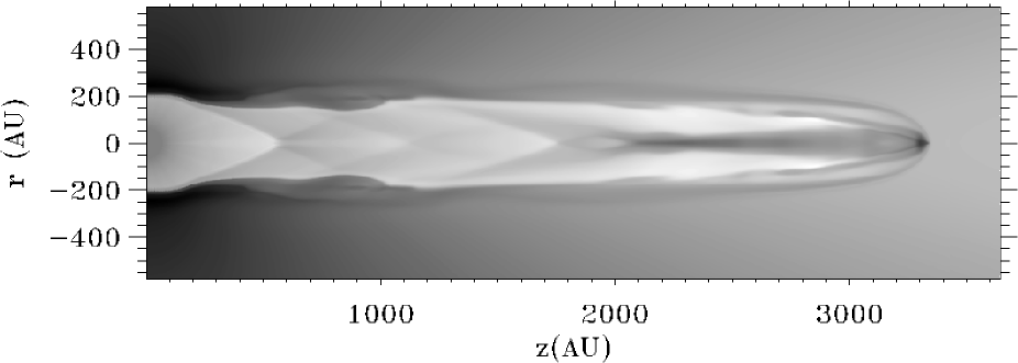
Figure 5: Comparison between runs B and C. The grey scales show $\log_{\rm 10}$ density contours for run B ($t=210$ years) and run C ($t=80$ years). In run C the ‘cool jet’ has been overtaken by the ‘hot jet’ and the whole structure is much narrower. The minimum/maximum pairs in units of cm^-3 are $(39.0,2.11\times 10^{6})$ and $(12.0,3.90\times 10^{6})$.

Obviously the velocity is an important parameter for setting the time scales of the different phases, but at the same time these results show that if there is substantial cooling a cool jet will form, even at outflow velocities as high as 450 km $\rm{s}^{-1}$. In fact for these high velocities the jet stays narrower; see Fig. 5.

3.4 The importance of cooling

To illustrate the importance of cooling for our collimation mechanism we performed simulations with the similar parameters, but differing a factor 100 in absolute density in both the outflow and the surroundings (runs D and E). The difference in density implies a factor $10^{4}$ less cooling in run E. The simulation was done on a grid of cylindrical spherical coordinates, using the Roe solver, and serves also a check that a different method produces similar results. In Fig. 6 we show the result for the two runs at the same time ($t=76$ years). Note first the lower value of the equator to pole density contrast, $q=50$, in these runs compared with the previous simulations. In run D one sees the same structure as described above, a momentum driven bubble with a jet forming at the tip. The jet is again very narrow, in fact hardly resolved. In run E we see a very different situation. The lack of cooling has caused the formation of an extensive bubble of hot shocked wind material. The inner shock is still somewhat aspherical, and a moderate degree of collimation occurs, but it is clearly of a different character than in run D. This is the type of collimation that was described by FM96. The comparison of these two runs shows that cooling is essential in creating these type of collimated outflows.

The results from run D also show that the inner shock region is sensitive to an instability in which ripples form along it. This behaviour is more noticeable in this simulation mainly because of the less diffusive character of the Roe solver method. The instability does not appear to have a large impact on the overall flow pattern. Run E and the simulations in FM96 display similar instabilities which lead to the formation of a hollow column of dense material, surrounding the jet beam. This collimating ‘chimney’ is not seen in runs A–D. This may be due to cooling making the walls stiffer to the instabilities or it may simply be a resolution effect. We do not believe we have adequate grid cells to resolve the post-shock cooling region which has $d_{\rm cool}<10^{13}$ cm [Blondin, Fryxell & Königl 1990] to the extent that the fate of instabilities can be accurately tracked. Regardless of the fate of the chimney in the context of these simulations the phenomena may be important in jet producing environments where radiative cooling is expected to be unimportant such as in active galactic nuclei.

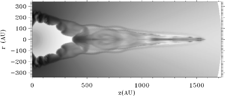
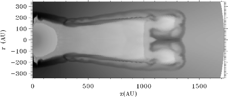
Figure 6: Comparison between runs D and E. The grey scales show $\log_{\rm 10}$ density contours for run D and run E (both at $t=76$ years). Run D is still completely radiative, and a cool jet has formed, while in run E an extensive hot bubble has developed. The minimum/maximum pairs in units of cm^-3 are $(412,1.01\times 10^{6})$ and $(0.195,6.65\times 10^{4})$

.

3.5 Jet temperature

Although the cooling time-scale for the material in the hot jet beam is longer than the time it takes to traverse the jet (in these simulations), the cooling time-scale is still relatively short. For run B, $t_{\rm cool}<500$ years at the base of flow. For run C, $t_{\rm cool}<50$ years at the base of flow. Since observed jet size scales are much larger than our computational grid ($L\approx 1$ pc) the material in the beam may be able to cool to lower temperatures on time-scales shorter than the jet lifetime. This tendency is apparent in run C where the cooling length $d_{\rm cool}=v_{\rm j}t_{\rm cool}<5\times 10^{16}$ cm. Fig. 5 clearly shows the presence of dense gas in the beam. This gas has cooled after having passed through the wind shock. We note also that we have used wind mass loss rates that are on the lower end of the observationally accepted spectrum [Natta 1989, Ceccarelli et al. 1997]. Higher mass loss rates mean high densities, shorter cooling time scales which for our models imply longer periods of cool jet collimation.

The issue of cooling the jets is an important point as they bear directly on the observational consequences of our model. The emission properties of a $T=10^{6}$ K plasma are obviously quite different than those for gas with $T<10^{4}$ K. For outflows from low mass stars current observations favour a cool jet scenario (Hartigan, private communication). There is however clear evidence for emission from ionized gas in the form of radio jets [Rodríguez 1995]. For high mass stars the situation is more complicated. The high velocities expected from their stellar winds almost ensures that any shocks in the wind will drive the gas to very high temperatures ($T>10^{6}$ K). Thus the thermal state of the gas is a critical diagnostic for our models. In future papers we plan to address this issue by examining the observational consequences of the various models using a ‘synthetic observations’ approach (cf. Frank & Mellema 1994). At the same time more observational work on the temperatures of the jets and outflows is needed.

4 The Effect of Wind Variability

The results from the previous section demonstrate that strong collimation can be achieved from purely hydrodynamic interactions between winds and protostellar environments. But to apply this model to young stars we must account for the time scales inherent to YSO jets and molecular outflows, assuming that jets are connected to the outflows [Chernin et al. 1994]. Recent deep exposure images of HH jets such as HH34 [Bally & Devine 1994] and HH46/47 [Heathcote et al. 1996] reveal multiple bow shock structures implying jet lifetimes of many thousands of years or more. In addition, the molecular outflows have dynamical lifetimes on the order of $10^{3}$ to $10^{5}$ years [Bachiller 1996]

If our simulations were allowed to run for such long periods we would expect the equatorial regions of the wind blown bubble to expand until the confining medium is eventually swept away. In the process the jet radius $r_{\rm j}$, which is of the order of the bubble’s equatorial radius $R_{\rm eq}$ would grow to an unacceptably large size. Thus if our model is to be viable it must account for the observed long lifetimes, small cross sections, and small collimating length scales of the jets. In this section we provide arguments that our model can account for these scales in a way which recovers additional aspects of YSO jets as well.

First we note that our simulations are simplified in that they do not include the presence of an accretion disk (of radial extend $\approx 100$ AU). In a realistic model it is unlikely that a dense but thin disk, offering a relatively small cross section and high inertia to the wind, would be pushed away. In addition for low mass stars it is likely that the wind itself may be originating in the inner regions of the disk [Shu et al. 1994]. Above and beyond the disk the bubble can be constrained in a number of ways. Magnetic fields threading the circum-protostellar environment can provide additional pressure restraining the growth of the bubble. If the field lines are anchored to a disk then magnetic tension can be quite effective in constraining the expansion of the bubble [Kwan & Tademaru 1995].

A more attractive and potentially more realistic means for stopping the equatorial growth of the bubble comes directly from the observations. As was mentioned above many HH jets show clear signs of variations in velocity along the jet beams. In the most extreme case the jet appears to be temporarily shut off, which explains the multiple bow-shock structures. In the HH34 superjet Bally & Levine [Bally & Devine 1994] find a periodicity in the beam of $\tau_{\rm j}=900/V_{\rm j300}$ years where $V_{\rm j300}$ is the jet velocity in units of 300 km $\rm{s}^{-1}$. Thus it is likely that $300<\tau_{\rm j}<900$ years. In addition smaller scale variations with periods $\tau<100$ years are seen in many HH jet beams (Morse, private communication). It is reasonable that the velocity variations in the jet beam are a measure of velocity variations in the source material of the jet. If this is the case then one should consider a scenario where the the wind-blown bubble is driven by a time-variable wind. In our simulations we did not include the effect of either gravity or the inward directed accretion flow. Both of these effects will decelerate the flow and constrain the bubble, particularly near the equator where the bubble radius is small so that the accretion velocity ($\propto R^{-0.5}$) and gravitational force density is high.

Figure 7: Evolution of spherical wind blown bubbles in accretion environment. Shown are the radius of 5 bubbles driven winds with different periods as a function of time. Solid line corresponds to a period of $P=10^{6}$ years. Dotted line: $P=500$ years. Dashed line: $P=400$ years. Dashed-dot line: $P=300$ years. Dashed-dot-dot line: $P=200$ years.

Thus it is possible that even though a bubble can be ‘launched’ by a protostellar wind the accretion ram pressure and gravitational deceleration may be able to significant slow, halt or even reverse the expansion of the bubble during a quiescent phase. To test this conjecture we developed a simple model for the interaction of a periodic stellar wind with an accreting environment. The model assumes spherical symmetry and strong radiative losses from the wind and ambient shocks so that we can use a thin shell approximation. The mass of the shell $M_{\rm s}$ and its radius $R_{\rm s}$. The equations for mass and momentum conservation for a shell of mass $M_{\rm s}$ and radius $R_{\rm s}$ are

$${dR_{\rm s}\over dt}=V_{\rm s}\,,\\$$ (14)

$${dM_{\rm s}\over dt}=4\pi{R_{\rm s}}^{2}\rho_{\rm w}(R_{\rm s})(V_{\rm w}-V_{\rm s})+$$

$$\quad\quad 4\pi{R_{\rm s}}^{2}\rho_{\rm a}(R_{\rm s})(V_{\rm s}+V_{\rm a})\,,$$ (15)

$${dM_{\rm s}V_{\rm s}\over dt}=4\pi{R_{\rm s}}^{2}\rho_{\rm w}(R_{\rm s})V_{\rm w}(V_{\rm w}-V_{\rm s})-$$

$$\quad\quad 4\pi{R_{\rm s}}^{2}\rho_{\rm a}(R_{\rm s})V_{\rm a}(V_{\rm s}+V_{\rm a})-{GM_{*}M_{\rm s}\over{R_{\rm s}}^{2}}\,,$$ (16)

[Volk & Kwok 1985]. Using the following definitions we can rewrite equations 15 and 16 in the form of a simple set of coupled ordinary differential equations (ODEs)

$$\rho_{\rm w}(R_{\rm s})={{\dot{M}_{\rm w}}\over 4\pi{R_{\rm s}}^{2}V_{\rm w}}\,,$$ (17)

$$\rho_{\rm a}(R_{\rm s})={{\dot{M}_{\rm a}}\over 4\pi{R_{\rm s}}^{2}V_{\rm a}(R_{\rm s})}\,,$$ (18)

$$V_{\rm a}(R)=\sqrt{{2GM_{*}\over{R_{\rm s}}}}\,,$$ (19)

$${dM_{\rm s}\over dt}={{\dot{M}_{\rm w}}\over V_{\rm w}}(V_{\rm w}-V_{\rm s})+{{\dot{M}_{\rm a}}\over V_{\rm a}}(V_{\rm s}+V_{\rm a})\,,$$ (20)

$${dV_{\rm s}\over dt}={1\over M_{\rm s}}\left[{\dot{M}_{\rm w}\over V_{\rm w}}(V_{\rm w}-V_{\rm s})^{2}-{\dot{M}_{\rm a}\over V_{\rm a}}(V_{\rm s}+V_{\rm a})^{2}-\right.$$

$$\quad\quad\left.{GM_{*}M_{\rm s}\over{R_{\rm s}}^{2}}\right]\,.$$ (21)

Equations 14, 20 and 21 together with initial conditions and a prescription for $V_{\rm w}=V_{\rm w}(t)$ define our model. For the wind velocity we take

$$V_{\rm w}(t)=V_{\rm wo}\left[{1\over 2}\left(1+\cos\left({2\pi t\over\tau_{\rm w}}\right)\right)+.01\right]\,,$$ (22)

and $\dot{M}_{\rm w}$ is kept constant. We also tried the case in which $\dot{M}_{\rm w}$ varies in the same way as $V_{\rm w}$, which gives similar results.

To solve our coupled set of ODEs we use a 4th order Runge-Kutta method with an adaptive step-size. The parameters for the wind ($\dot{M}_{\rm w}$ and $V_{\rm wo}$) and the environment are the same as in Model A, see Table 1. The initial radius at which the integration begins is $R_{\rm so}=6.5\times 10^{13}$ cm. The initial mass of the shell $M_{\rm so}$ was taken to be the amount of circumstellar mass originally contained in the volume $4\pi R_{\rm so}^{3}/3$. The initial velocity was arbitrarily taken to be $V_{\rm so}=5V_{\rm a}(R_{\rm so})$. The assumption is that before the start of the integration, the bubble was set in motion, perhaps by an energetic episodic outburst from the protostar. This initial condition gives a total energy in the shell of $10^{40}$ ergs which is more than five orders of magnitude less than what is released in a typical FU Orionis outburst [Hartmann & Kenyon 1996].

We calculated the evolution of the bubble for the case where the wind is constant as well as for four time-dependent wind models with periods $\tau_{\rm w}=$500, 400, 300 and 200 years. The results are shown in Fig. 7. For the constant wind the bubble expands monotonically although it does experience changes in velocity due to accretion ram pressure and gravitational forces. When the wind is allowed to vary these forces produce dramatic changes in the bubble’s evolution. For all four variation periods we see that the expansion of bubble can be reversed ($V_{\rm s}<0$) for some time. For longer periods the bubble gains enough momentum before the wind enters a minimum to either continue a slow expansion ($\tau_{\rm w}=500$ years) or maintain a constant average radius ($\tau_{\rm w}=400$ years). For shorter periods the bubble is “crushed” during the wind’s quiescent phase by the inward directed forces. Note that we end the calculation if the shock radius $R_{\rm s}$ became smaller than $10^{12}$ cm.

Two important points should be kept in mind. Firstly, the results are sensitive to the initial conditions. Whether a bubble expands, oscillates or collapses is a strong function of the initial position $R_{\rm so}$ and velocity $V_{\rm so}$ of the shell, and the momentum input of the wind. But for each set of $(R_{\rm so},V_{\rm so})$ it is always possible to find parameters for the wind which will lead to one of these three solutions. The second point concerns the extension of this model to non-spherical bubbles. Our simulations show that the equatorial radius in an aspherical bubbles is always less than that derived from a 1-D calculation (FM96). Thus the results shown in Fig. 7 should be taken as an upper limit to the equatorial size scale of the bubble and hence the scale of the collimation region.

From these results we conclude that that, in principle, time varying winds can produce wind-blown bubbles whose size never increases beyond some upper limit. If these bubbles produce jets through the hydrodynamic mechanisms described in Section 3, the model age and collimation scales can be made consistent with observations. We imagine that during a periodic increase in mechanical luminosity the YSO will begin driving a bubble which in turn produces collimated jets. As the wind speed varies the bubble either oscillates around some average radius (producing variations in the jet beam) or it collapses entirely. Jet production begins again when the momentum in the wind has increased enough to produce another bubble.

These oscillating bubbles are likely to be subject to Rayleigh-Taylor instabilities, especially around the turn-around time. How this affects the bubble structure and jet formation is difficult to say on the basis of the simple one-dimensional model. It is a potential problem to this scenario which we intend to study in future papers.

5 Conclusions

The results presented in this paper show that the collimation of an outflow from a central object through the interaction with a surrounding toroidal density distribution can be very efficient. In FM96 we addressed the case of non-cooling flows and showed that these can be collimated much more efficiently than one would anticipate from a simple analysis. Here we included the effects of cooling and found that some of the effects described in FM96 still hold, but that there is an additional collimating effect producing converging, collimated flows at the poles of the wind blown bubble. This effect appears only to operate under cooling conditions, presumably because only then is the distance between the wind shock and contact discontinuity small enough to constrain shocked wind material into a narrow converging flow focused towards the axis. The cooling also allows the wind shock to take on more prolate geometries which enhances the flow focusing.

When cooling is effective the interaction between a spherical outflow and a toroidal environment is found to consist of two phases. Initially the bubble is nearly completely radiative and the focusing of the flow at the top of the bubble creates a dense, cool jet. The basic mechanism for this is the same one that was studied by CTTR although the circumstances here are somewhat different from the ones described there. The collimation achieved is very good, the jet is an order of magnitude narrower than the radiative bubble. We call this this the ‘cool jet’.

This ‘cool jet’ phase is followed by a ‘hot jet’ which also forms at the top of the bubble. In this second case the collimation mechanism is similar to the one described in FM96. This second jet starts forming when the cooling at the top of the bubble becomes less efficient due to lower values of the density there. The hot jet follows the same path as the cool one and eventually overtakes it. The collimating processes consist essentially of focusing at the inner shock (including supersonic post-shock flow), and the inertia of surrounding material.

The difference between the cool and hot jet phases may be particularly relevant when comparing low mass and high mass star formation and their jets. High mass stars are likely to possess high velocity winds; when these are shocked cooling is likely to be ineffective at the high post-shock temperatures. The jets which formed this way may be fast and hot. The shocks may also produce significant non-thermal radiation via the first-order Fermi process [Ip 1995, Henriksen, Ptuskin & Mirabel 1991]. Such non-thermal emission has already been observed. Reid et al. [Reid et al. 1995] found strong synchrotron emission arising at the centre of a linear chain of maser sources. Their interpretation is that the wind from a massive star is being redirected via shocks into a jet which drives the maser sources. This closely matches what we predict from our model. Recent high resolution images show the synchrotron emission actually appears as a two sided jet emanating from the geometric centre of the two maser flows [Wilner et al. 1997].

We also showed that it is, in principle, possible to obtain long-lived jets with the correct collimation scales if the wind is variable. In that case the bubble can collapse back towards the star during the wind’s quiescent phase; new jets form during the next active outburst phase. This may naturally explain the knots and multiple bow-shocks observed in some HH jets.

The current investigation completes our work on the fundamental hydrodynamics of the time-dependent hydrodynamic collimation. The next step will involve using more realistic proto-circumstellar environments and including relevant diagnostics to make a comparison with observations. This latter point is crucial and must be carried out carefully. The main difference between our models and those which rely on collimation through MHD effects is the presence of strong shocks. In our our models oblique shocks are essential for redirecting an uncollimated wind into a jet. The tracers of these shocks and the absorbing effect of the dense surrounding medium must be calculated carefully if realistic comparisons between theory and observations are to be made.

References

- [Bachiller 1996] Bachiller R., 1996, ARAA, 34, 111
- [Bachiller, Tafalla, & Cernichado 1994] Bachiller R., Tafalla M., Cernichado J., 1994, ApJ, 432, L127
- [Bally & Devine 1994] Bally J., Devine D., 1994, ApJ, 428, L65
- [Blondin, Fryxell & Königl 1990] Blondin J. M., Fryxell B. A., Königl A., 1990, ApJ, 360, 370
- [Burrows et al. 1996] Burrows C. J. et al., 1996, ApJ, 473, 437
- [Cantó & Rodriguez 1980] Cantó J., Rodríguez L. F., 1980, ApJ, 239, 982
- [Cantó, Tenorio-Tagle & Różyczka 1988] Cantó J., Tenorio-Tagle G., Różyczka M., 1988, A&A, 192, 287 (CTTR)
- [Ceccarelli et al. 1997] Ceccarelli C., Haas M. R., Hollenbach D. J., Rudolph A. L., 1997, ApJ, 476, 771
- [Chernin et al. 1994] Chernin L. M., Masson C. R., Dal Pino E. M., Benz W., 1994, ApJ, 426, 204
- [Dalgarno & McCray 1972] Dalgarno A., McCray R., 1972, ARAA, 10, 375
- [Eichler 1982] Eichler D., 1982, ApJ, 263, 571
- [Frank & Mellema 1994] Frank A., Mellema G., 1994, ApJ, 430, 800
- [Frank & Mellema 1996] Frank A., Mellema G., 1996, ApJ, 472, 684 (FM96)
- [Frank & Noriega-Crespo 1994] Frank A., Noriega-Crespo A., 1994, A&A, 290, 643
- [Frank, Balick & Livio 1996] Frank A., Balick B., Livio M., 1996, ApJ, 471, L53
- [Hartigan et al. 1992] Hartigan P., Morse J. A., Heathcote S., Cecil G., 1992, ApJ, 414, L121
- [Hartigan et al. 1996] Hartigan P., Reipurth B., Morse J. A., Heathcote S., Bally J., Heathcote S., Schwartz R. D., 1996, BAAS, 28, 885
- [Harten 1983] Harten A., 1983, J. Comp. Phys., 49, 357
- [Hartmann & Kenyon 1996] Hartmann L., Kenyon S., 1996, ARAA, 34, 207
- [Hartmann, Calvet, & Boss 1996] Hartmann L., Calvet N., Boss A., 1996, ApJ, 464, 387
- [Heathcote et al. 1996] Heathcote S., Morse J. A., Hartigan P., Reipurth B., Schwartz R. D., Ball J., Stone J. M., 1996, AJ, 112, 1141
- [Henriksen, Ptuskin & Mirabel 1991] Henriksen R., Ptuskin V., Mirabel I., 1991 A&A, 248, 221
- [Icke 1988] Icke V., 1988, A&A, 202, 177
- [Icke et al. 1992] Icke V., Mellema G., Balick B., Eulderink F., Frank A. 1992, Nat, 355, 524
- [Ip 1995] Ip W. H., 1995, A&A, 300, 283
- [Königl 1982] Königl A., 1982, ApJ, 261, 115
- [Königl 1989] Königl A., 1989, ApJ, 342, 208
- [Königl & Ruden 1993] Königl A., Ruden S. P., 1993, in Levy E. H., Lunine J. I., eds, Protostars and Planets III. Univ. of Arizona Press, Tucson, AZ. p. 641
- [Koo & McKee 1992] Koo B., McKee C. F., 1992, ApJ, 388, 103
- [Kraemer et al. 1997] Kraemer K. E., Jackson J. M., Paglione T. A. D., Bolatto A. D., 1997, ApJ, 478, 614
- [Kwan & Tademaru 1995] Kwan J., Tademaru E., 1995, ApJ, 454, 382
- [Li & Shu 1996] Li Z., Shu F., 1996, ApJ, 472, 211
- [Lucas & Roche 1997] Lucas P. W., Roche P. F., 1997, MNRAS, in press
- [Matsumoto, Hanawa & Nakamura 1997] Matsumoto T., Hanawa T., Nakamura F., 1997, ApJ, 478, 569
- [Mellema 1996] Mellema G., 1996, in Kundt W. R., ed, Jets from Stars and Galactic Nuclei. Springer, Berlin. p. 149
- [Mellema, Eulderink & Icke 1991] Mellema G., Eulderink F., Icke V., 1991, A&A, 252, 718
- [Morse et al. 1992] Morse J. A., Hartigan P., Cecil G., Raymond J. C., Heathcote S. 1992, ApJ, 339, 231
- [Natta 1989] Natta A. 1989, in Reipurth B., ed, Low Mass Star Formation and Pre-Main Sequence Objects. ESO, Garching bei München. p. 365
- [Pelletier & Pudritz 1992] Pelletier G., Pudritz R. E., 1992, ApJ, 394, 117
- [Peter & Eichler 1995] Peter W., Eichler D., 1995, ApJ, 438, 244
- [Peter & Eichler 1996] Peter W., Eichler D., 1996, ApJ, 466, 840
- [Pudritz 1991] Pudritz R. E., 1991, in Lada C. J., Kylafis N. D., eds, The Physics of Star Formation and Early Stellar Evolution. Kluwer, Dordrecht. p. 365
- [Raga & Cantó 1989] Raga A. C., Cantó J., 1989, ApJ, 344, 404
- [Raga & Kofman 1992] Raga A. C., Kofman L., 1992, ApJ, 386, 222
- [Reid et al. 1995] Reid M. J., Argon A. L., Masson C. R., Menten K. M. Moran J. M., 1995, ApJ, 443, 238
- [Rodríguez 1995] Rodríguez L. F., 1995, RevMexAA Ser. Conf, 1, 1
- [Romanova et al. 1996] Romanova M., Ustyugova G., Koldoba A., Chechetkin V., Lovelace R., 1996, preprint
- [Ryu et al. 1995] Ryu D., Brown G. L., Ostriker J. P., Loeb A., 1995, ApJ, 452, 364
- [Stone & Norman 1994a] Stone J. M., Norman M. L., 1994, ApJ, 413, 198.
- [Shu et al. 1994] Shu F., Najiata J., Ostriker E., Wilkin F., Ruden S., Lizano S., 1994, ApJ, 429, 781
- [Tenorio-Tagle, Cantó & Różyczka 1988] Tenorio-Tagle G., Cantó J., Różyczka M., 1988, A&A, 202, 256 (TTCR)
- [Tereby, Shu & Cassen 1984] Tereby S., Shu F., Cassen P., 1984, ApJ, 286, 529
- [cf. Yorke, Bodenheimer & Laughlin 1993] Yorke H. W., Bodenheimer P., Laughlin G., 1993, ApJ, 411, 274
- [Volk & Kwok 1985] Volk K., Kwok S., 1985, A&A, 153, 79
- [Wilner et al. 1997] Wilner D. J., Reid M. J., Menten K. M., Moran J. M., 1997, in Malbet F., Castets A., eds., Poster proceedings of IAU Symp. 182 on Herbig–Haro Objects and the Birth of Low Mass Stars. Obs. de Grenoble, Grenoble. p. 193