Simulations of superhumps and superoutbursts

Abstract

We numerically study the tidal instability of accretion discs in close binary systems using a two-dimensional SPH code. We find that the precession rate of tidally unstable, eccentric discs does not only depend upon the binary mass ratio $q$. Although the (prograde) disc precession rate increases with the strength of the tidal potential, we find that increasing the shear viscosity $\nu$ also has a significant prograde effect. Increasing the disc temperature has a retrograde impact upon the precession rate.

We find that motion relative to the binary potential results in superhump-like, periodic luminosity variations in the outer reaches of an eccentric disc. The nature and location of the luminosity modulation is a function of $\nu$. Light curves most similar to observations are obtained for $\nu$ values appropriate for a dwarf nova in outburst.

We investigate the thermal-tidal instability model for superoutburst. A dwarf nova outburst is simulated by instantaneously increasing $\nu$, which causes a rapid radial expansion of the disc. Should the disc encounter the $3:1$ eccentric inner Lindblad resonance and become tidally unstable, then tidal torques become much more efficient at removing angular momentum from the disc. The disc then shrinks and $\dot{M}_{\rm d}$ increases. The resulting increase in disc luminosity is found to be consistent with the excess luminosity of a superoutburst.

1 Introduction

In a previous paper (Murray 1996, hereafter Paper I) we described a two dimensional smoothed particle hydrodynamics (SPH) code specifically designed for thin disc problems. We showed that the standard SPH artificial viscosity term introduces a kinematic shear viscosity, $\nu$, into a disc simulation that can be accurately estimated analytically by taking the SPH equation of motion to the continuum limit. For a two dimensional SPH code with the standard cubic spline kernel one obtains

$$\nu=\frac{1}{8}\,\zeta\,c\,h.$$ (1)

where $\zeta$ is the coefficient of the linear artificial viscosity term, $c$ is the sound speed, and $h$ is the SPH smoothing length (which has been kept fixed in all calculations described herein). Equation 1 was verified with axisymmetric ring-spreading calculations, and by comparing the stationary end state of a simulation of a disc in a binary with axisymmetric theory.

Two simulations of discs in low mass ratio $(q=3/17)$ binary systems evolving under steady mass transfer from the secondary were described. In agreement with calculations in Whitehurst (1988) and Hirose & Osaki (1990), the discs encountered the binary system’s $3:1$ eccentric inner Lindblad resonance (see Lubow 1991a). As a result, both discs became considerably eccentric and, as seen in the inertial frame, precessed slowly in the prograde direction. Whitehurst (1988) proposed that the superhump phenomenon seen in some short period cataclysmic variables was the signature of a precessing, eccentric disc. Indeed, in the simulations described in Paper I approximately ten to twenty per cent of the total luminosity from the eccentric disc was modulated at the frequency of the motion of the disc’s semi-major axis in the binary potential.

In this paper we describe a more thorough numerical investigation of the so called tidal instability of accretion discs in close binary systems. Simulations for a range of binary mass ratios, disc temperatures, and shear viscosities are described in order to illustrate the relative importance of these parameters in determining whether discs are tidally unstable. Eccentricity growth rates and disc precession rates are compared with observations and with analytical results obtained by Lubow (1991a, 1992). We go on to demonstrate that tidal instability can not only explain the superhumps seen in SU UMa systems, but also provide a long-term increase in energy dissipation in the disc that is consistent with the excess luminosity of SU UMa superoutbursts. Simulations described here provide considerable support for the thermal-tidal instability model for superoutburst proposed by Osaki (1989).

In section 2 we briefly outline our current understanding of SU UMa systems, superhumps and superoutbursts. In section 3.1 we discuss our numerical scheme, focusing on alternative methods of introducing shear viscosity into disc calculations. Then in section 3.2 we detail the assumptions and parameter settings used in the various simulations. Section 4 is devoted to numerical results of superhump simulations (4.1), and superoutburst simulations (4.2). Our major conclusions are summarised in section 5.

2 Preamble

2.1 The SU Ursae Majoris systems

Cataclysmic variable (CV) stars are semi-detached binary systems, with a white dwarf as the detached component (primary), and a low mass star as the contact component (secondary). For a comprehensive review of the observations and theory of CVs see Warner (1995). Typically a few tenths of a solar mass, the secondary star loses mass to the more massive white dwarf via Roche lobe overflow. In the absence of strong magnetic fields, the transferred gas forms an accretion disc around the white dwarf. CVs display a wide variety of eruptive behaviours, and non-magnetic systems are phenomenologically categorised on this basis.

Dwarf novae are CVs that undergo luminosity increases (outbursts), typically of 2–5 magnitudes, which last a few days and recur on a time-scale of days to weeks. The SU Ursae Majoris (SU UMa) systems form a subclass of dwarf novae that also exhibit a related but distinct phenomenon, called superoutburst. These eruptions are approximately one magnitude brighter than normal outbursts and last as long as a couple of few weeks rather than just a few days. The accretion disc has been found to be the source of the excess luminosity of both normal outbursts and superoutbursts. Because superoutbursts often very closely follow a normal outburst, and because of similarities in the rises to maximum, it is likely that superoutbursts are triggered by normal outbursts.

For a recent review of the observational details of the superoutburst phenomenon, the reader is once again referred to Warner (1995). Here we merely highlight a few relevant points. Firstly, it appears that all SU UMa systems have short periods and that all dwarf novae with short periods are SU UMa systems. Thorstensen et al. (1996) tabulated the orbital periods for 26 SU UMa systems. Of these, TU Men had the longest orbital period with $P_{\rm b}=169.34\,{\rm min}$. Even TU Men’s period is short relative to the orbital periods of ordinary dwarf novae. Warner (1995) made the remark that all dwarf novae with periods $P_{\rm b}\la 3\,{\rm hrs}$ are eventually identified as SU UMa systems.

The shorter a CV’s orbital period is, the smaller its binary mass ratio, $q={M_{\rm sec}}/{M_{\rm pri}}$, is expected to be. Those dwarf novae with periods less than three hours (i.e. the SU UMa systems) are thought to have $q\la 0.3$.

2.2 Superhumps

Superhumps are large amplitude modulations of a CV’s optical light curve. Typically, the superhump period, $P_{\rm sh}$, is a few per cent longer than the binary period. Until recently, superhumps had been seen only in SU UMa systems during their superoutburst phase. This is no longer the case. Patterson et al. (1995) observed the superhumps in the SU UMa system V1159 Orionis to persist well after superoutburst had ended. Modulations tentatively identified as superhumps have also been observed in several other short period cataclysmic variables (see Patterson & Richman 1991, Retter, Leibowitz & Ofek 1997) that don’t exhibit classic dwarf novae activity.

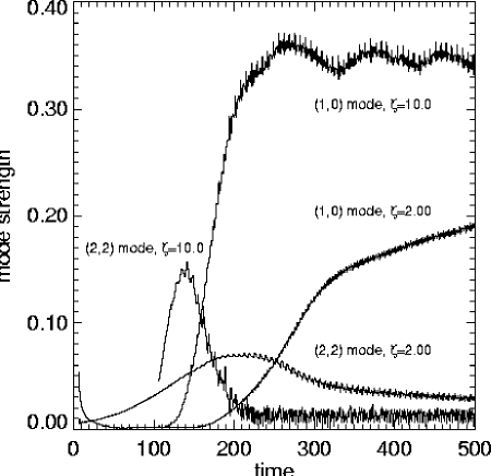
Figure 9: Strengths of the eccentric $(1,0)$ and the tidal $(2,2)$ modes for the superoutburst simulation ($\zeta=10.0$) and for run 6 ($\zeta=2.00$). Time (in $\Omega_{\rm b}^{-1}$) is measured from the beginning of run 6. Thus the superoutburst simulation starts at $t=100.00\,\Omega_{\rm b}^{-1}$.

Thorstensen et al. plotted the fractional superhump period excess for 26 SU UMa systems as a function of $P_{\rm b}$ (their figure 9), and obtained a line of best fit

$$\frac{P_{\rm sh}-P_{\rm b}}{P_{\rm b}}=-0.0344+(0.0382\,{\rm hr}^{-1})\,P_{\rm b}.$$ (2)

With $P_{\rm b}$ thought to be an increasing function of $q$, we can infer that the superhump period is also dependent upon the binary mass ratio. Significantly, the superhump period excess does not go to zero with the binary period. This empirical relationship suggests that in the limit of very small $q$, the superhump period would be shorter than the binary period.

For a given system $P_{\rm sh}$ is commonly found not to be completely stable but may in fact decrease slightly over the course of a single superoutburst (see e.g. Patterson et al. 1995).

2.3 The Thermal-Tidal Instability Model for Superoutbursts

Osaki (1989) proposed a model for SU UMa superoutbursts that incorporates the thermal instability model for normal dwarf nova outbursts, and a tidal instability that induces the accretion disc to become eccentric. The details of the thermal instability model can be found in Cannizzo (1993a). Central to the model is the hypothesis that angular momentum transport is much more efficient on the hot branch of the limit-cycle than on the cold branch. A dwarf nova outburst then is a period of enhanced mass flux $\dot{M}_{\rm d}$ through the disc. Cannizzo (1993b) found that a disc with Shakura-Sunyaev viscosity parameters $\alpha_{\rm hot}=0.2$ and $\alpha_{\rm cold}=0.01$ best reproduced the observed dwarf nova outbursts of SS Cygni.

The tidal instability is due to the $3:1$ eccentric inner Lindblad resonance (see Lubow 1991a). Only in systems with small binary mass ratio $(q\la 0.3)$ can the disc extend to the resonant radius, and then only if angular momentum transport in the disc is reasonably efficient. It should only be possible to excite the resonance in short period CVs that are on the hot branch (whether permanently or temporarily) of the thermal limit-cycle.

In Osaki’s so called thermal-tidal instability model for superoutbursts, each normal outburst causes a net radial expansion of the disc. When the disc expands sufficiently it encounters the resonance and becomes eccentric. Osaki proposed that in its eccentric state, the disc would be subject to greatly enhanced tidal torques that increased the mass flux, $\dot{M}_{\rm d}$, through the disc and therefore increased the disc luminosity, explaining why superoutbursts are significantly brighter than normal outbursts. In the inertial frame, the eccentric disc exhibits a slow prograde precession, and superhumps are explained as a beat phenomenon between the motion of the disc and the motion of the binary. The thermal-tidal instability model is reviewed in Osaki (1996).

3 Numerical Method

3.1 SPH

The two-dimensional smoothed particle hydrodynamics (SPH) code used here has already been described in Paper I. In that paper, we demonstrated the code’s ability to reliably model an accretion disc with a given kinematic shear viscosity, $\nu$. By taking the equations of motion for the SPH particles to the continuum limit, one finds that the standard SPH artificial viscosity term generates a force per unit mass

$${\bf{a}}_{\rm v}=\frac{\zeta h\kappa}{2\Sigma}\,({\bf{\nabla}}\cdot(c\Sigma{\bf{S}})+{\bf{\nabla}}(c\Sigma{\bf{\nabla}}\cdot{\bf{v}})).$$ (3)

Here $\zeta$ is the coefficient of the linear SPH artificial viscosity term, $h$ is the smoothing length, $\Sigma$ is the disc column density, ${\bf{v}}$ is the velocity, and

$$S_{ab}=\frac{{\rm\partial}v_{a}}{{\rm\partial}x_{b}}+\frac{{\rm\partial}v_{b}}{{\rm\partial}x_{a}}$$ (4)

is the deformation tensor. In two dimensions

$$\kappa=\frac{\pi}{4}\,\int_{0}^{\infty}{r^{2}}\,\frac{{\rm d}W}{{\rm d}r}\,dr.$$ (5)

For the standard cubic spline kernel, $\kappa=\frac{1}{4}$. If the sound speed is only slowly varying in space, the SPH artificial viscosity produces a shear viscosity with magnitude given by equation 1. In regions where the dilatation is non-zero, a bulk viscosity is also produced.

In the inner accretion disc, orbits are approximately circular and the shear term dominates the dissipation. In the outer disc where the tidal influence of the secondary is stronger, the bulk term is more important. The radial extent of the disc depends upon the relative magnitudes of the shear and bulk viscosities (Papaloizou and Pringle 1977)). $r_{\rm m}$, the mean radius of the largest simply periodic test particle orbit that doesn’t intersect other such orbits of smaller radius (Paczyński 1977), is a simple estimator of the boundary between shear and bulk viscosity dominated regions of the disc.

The standard linear SPH artificial viscosity term includes shear and bulk viscosity in a fixed ratio. One can derive SPH interpolant estimates of $\nabla^{2}\,{\bf{v}}$, and hence include independent shear and bulk viscosity terms in the SPH equations. Two possible SPH formulations were introduced by Flebbe et al. (1994) and Watkins et al. (1996). However these methods require two levels of interpolation to generate the second derivatives of the velocity and so smooth information over a larger region. Furthermore, in these formulations, the forces between two particles are not antisymmetric and along the particles’ line of centres. As a result, angular momentum is only conserved at a global level to an accuracy dictated by the interpolation scheme. As we wish to use the dissipation terms to transport angular momentum it is highly desirable that angular momentum be conserved as precisely as possible. With the dissipation term we use, linear and angular momentum are conserved to machine accuracy at the particle level.

In standard SPH, there is a ‘viscous switch’ that sets the viscous force between two particles to zero if they are receding from one another. This is to ensure that dissipation only occurs in regions of compression. For our disc SPH code, the switch is disabled. The quadratic term in the standard SPH artificial viscosity formulation is not used. This term always produces a repulsive force between two particles and so causes problems at the outer edge of the disc where particles are flung to very large radii.

3.2 Simulation Details

We use the scalings of Lin and Pringle (1976), where the total system mass $M$, the binary orbital angular velocity $\Omega_{\rm b}$, and the interstellar separation $d$, are all set to one.

We approximate the gravitational potential of the binary to be that of two point masses in circular orbit of radius $d$ about each other. We have an open inner boundary condition, i.e. there is a hole in the computational domain of radius $r_{\rm wd}$ centred on the position of the primary (point mass). At the end of each time step particles lying within this circle are removed from the simulation. In all simulations described here we use $r_{\rm wd}=0.02\,d$. Particles that end a time step either within the secondary star’s Roche lobe or a distance $r>0.9\,d$ from the primary’s centre of mass are also deleted.

An isothermal equation of state (i.e. constant sound speed c) is used. We also set the SPH artificial viscosity parameter $\zeta$ to be constant, so that the kinematic and bulk viscosities will be constant. As in Paper I, energy dissipation in the disc is calculated using the SPH energy equation (see their equation 17).

Mass is added to the calculation in one of two ways. If we wish to incorporate the mass transfer stream in the simulation we add a single particle per time step $\Delta t$ at the inner Lagrangian point. In principle, the stream boundary conditions at $L_{1}$ are a function of the binary mass ratio $q$ (see Lubow and Shu 1975). In practice we always added particles with an initial speed $v_{\rm inj}=0.1\,d\,\Omega_{\rm b}$, in a direction $0.367$ radians prograde of the binary axis. If we do not wish to include the mass transfer stream in the calculation we simply add one particle per time interval $\Delta t$ in a circular Keplerian orbit of radius $r_{\rm c}$. Standard practice is to choose $r_{\rm c}$ to be the circularisation radius, which is again a function of the mass ratio. For these simulations, when we did add particles in circular orbit, it was at $r_{\rm c}=0.1781\,d$. Unless specifically stated, we always chose the interval between particle addition to be $\Delta t=0.01\,\Omega_{\rm b}^{-1}$

As we have an isothermal equation of state and constant $\nu$, the fluid equations are independent of the mass scaling. In other words our choice of particle mass has no effect upon the simulation outcome beyond scaling the surface density. In every simulation then, we chose the particle mass to give us a mass transfer rate from the secondary star of $10^{-9}\,M_{\odot}{\rm yr}^{-1}$ assuming $P_{\rm b}=0.063121$ days (the period for OY Car).

4 Results

4.1 Tidal Instability and Superhumps

We have completed twelve simulations in which we began with zero initial mass and followed the viscous evolution of the disc under steady mass addition. The results are summarised in Table 1. Note that runs 4 and 5 were previously described in Section 4 of Paper I as simulations 1 and 2 respectively. In run 6, the shear viscosity $\nu=5\times 10^{-5}d^{2}\,\Omega_{\rm b}$. In runs 7,8 and 12, $\nu=2.5\times 10^{-5}d^{2}\,\Omega_{\rm b}$. In all the other calculations, $\nu=2.5\times 10^{-4}d^{2}\,\Omega_{\rm b}$.

We followed each calculation for a time (see column 4 of the table) that was sufficient for us to determine whether the disc would become eccentric or not, and also long enough for us to accurately measure precession periods. For example, as it was apparent that run 1 had reached an essentially steady state, and as it was clear that the disc would not become eccentric, the simulation was terminated at $t=1652.05\,\Omega_{\rm b}^{-1}$.

Computing requirements also dictated the length of various simulations. The total number of particles in a disc at steady state is proportional to the rate at which particles are added to the disc, and inversely proportional to the viscosity. Of course the computing time increases with the number of particles. On the other hand, if we wished to follow the viscous evolution of a relatively inviscid disc, we are required to follow the calculation for many binary orbital periods. Hence when we reduced $\nu$ by a factor 10 in runs 7 and 8, we also reduced the rate of particle addition (but not mass addition) to the disc to one sixth the standard value.

Most of the simulations result in eccentric, precessing discs. Our technique for determining the period of the disc’s motion in the binary frame $P_{\rm d}$, differs from the method used in Paper I. There we measured the motion of the disc’s centre of mass and obtained a mean value for $P_{\rm d}$. We estimated an uncertainty in our figure from the standard deviation of the data. However, it is possible to identify $P_{\rm d}$ in simulation ‘luminosity’ data as well. At regular time intervals ($0.01\,\Omega_{\rm b}^{-1}$) we record the rate at which energy is being dissipated in various regions of the disc, to obtain time series that can be analysed for periodicities in the same manner as observational data. We loosely equate the energy dissipation rate to luminosity. These time series, which we shall refer to as ‘simulation light curves’, are illustrated in figure 6 and discussed later in this section.

To obtain a mean period $P_{\rm d}$ we simply Fourier transform the simulation light curve. As noted in Paper I, simulation light curves from the entire disc are made quite noisy by the action of a small number of particles releasing large amounts of energy in the inner disc. Thus we used light curves obtained from disc regions at radii $r>0.20\,d$. The Fourier spectrum from run 10 is shown in Fig. 1. Clearly there is only one frequency in the data at 215 cycles per $1400.00\,\Omega_{\rm b}^{-1}$. The other peaks are simply higher harmonics. The spectra from the other runs are similarly unambiguous, with the peaks being only one or two cycles wide. The values given for ${P_{\rm d}}/{P_{\rm b}}$ for runs 4 and 5 are consistent with, but more precise than, the values given in Paper I.

Table 1: Summary of simulations and their basic results

Run	$q$	$c$	$\zeta$	Time	${P_{\rm d}}/{P_{\rm orb}}$	${P_{\rm d}}/{P_{\rm orb}}$	$\lambda_{\rm t}$	$\lambda_{\rm m}$	final $S_{(1,0)}$	$t_{\rm inst}$
		$d\,\Omega_{\rm b}$		$\Omega_{\rm b}^{-1}$	(mean)	(max)	$\Omega_{\rm b}$	$\Omega_{\rm b}$		$\Omega_{\rm b}^{-1}$
1	0.29	0.02	10.00	1652.05	no oscillation	—	—	—	$0.001\pm 0.001$	—
2	0.25	0.02	10.00	2000.00	$1.128\pm 0.004$	e	$0.26\pm 0.01$	$0.012\pm 0.001$	$0.15\pm 0.01$	729.81
3	0.25	0.06	3.333	2000.00	$1.073\pm 0.003$	$1.099\pm 0.006$	0.3	$0.018\pm 0.001$	$0.53\pm 0.01$	181.24
4	3/17	0.02	10.00	1000.00	$1.079\pm 0.009$	f	$0.10\pm 0.01$	$0.046\pm 0.002$	$0.31\pm 0.02$	367.88
5	${3/17}^{a}$	0.02	10.00	1000.00	$1.074\pm 0.009$	f	g	$0.058\pm 0.002$	$0.35\pm 0.03$	63.66
6	${3/17}^{a}$	0.02	2.000	870.20	$1.064\pm 0.001$	$1.074\pm 0.001$	g	$0.052\pm 0.004$	${0.220}^{h}$	183.75
7	${3/17}^{b}$	0.02	1.000	6374.76	$1.049\pm 0.001$	$1.070\pm 0.001$	g	$0.020\pm 0.004$	$0.27\pm 0.01$	689.28
8	${3/17}^{a,b}$	0.02	1.000	8551.08	$1.047\pm 0.001$	$1.069\pm 0.002$	g	$0.025\pm 0.003$	$0.29\pm 0.01$	480.66
9	1/9	0.02	10.00	1618.77	$1.053\pm 0.003$	f	0.059 – 0.066	$0.036\pm 0.002$	$0.39\pm 0.05$	198.59
10	1/9	0.06	3.333	2000.00	$1.036\pm 0.002$	$1.051\pm 0.004$	0.06 – 0.07	$0.0190\pm 0.0005$	$0.52\pm 0.02$	181.24
11	1/19	0.02	10.00	1436.20	no oscillation	—	—	—	$0.001\pm 0.001$	—
12	${1/19}^{a}$	0.02	1.000	1000.00	$1.018\pm 0.001$	f	0.0027	$0.018\pm 0.002$	${0.232}^{h}$	342.19

^a mass added in circular orbit at radius $r_{\rm c}$.

^b particles added singly every $\Delta t=0.06\,\Omega_{\rm b}^{-1}$

^e period is stable to within uncertainty in measurement of ${P_{\rm d}}/{P_{\rm orb}}$.

^f ${P_{\rm d}}$ increases over first 10 or so periods.

^g use the same value as in run 4.

^h eccentricity increasing at a rate $0.0001$ per scaled time unit.

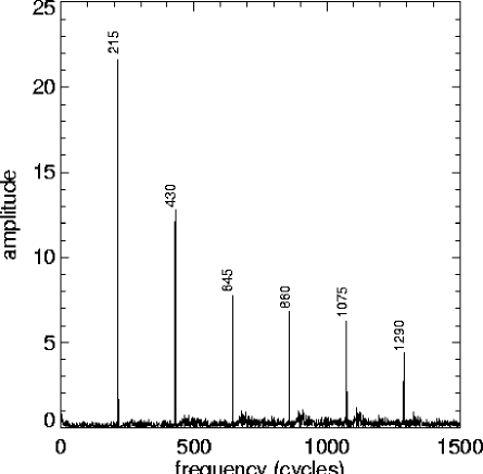
Figure 1: Fourier transform of the outer disc $(r>0.20\,d)$ light curve from run 10. The time series covers a $1400.00\,\Omega_{\rm b}^{-1}$ time period with a resolution of $0.01\,\Omega_{\rm b}^{-1}$. We thus estimate $P_{\rm d}=1400.00/215\,\Omega_{\rm b}^{-1}$.

The mean values of ${P_{\rm d}}/{P_{\rm b}}$ are listed in column 6 of Table 1. As noted in Paper I (see their Table 3), for a given mass ratio $q$, different authors have obtained a range of values for ${P_{\rm d}}/{P_{\rm b}}$. One can append the results of three dimensional simulations completed by Whitehurst (1994) to that table. Because everybody had used their own numerical scheme, it was not clear whether the differences were physical or numerical.

From Table I however it is now apparent that ${P_{\rm d}}/{P_{\rm b}}$ is not simply a function of $q$. It is also influenced by the temperature and dissipation in the disc. For example the only difference between runs 9 and 10 is a factor 3 increase in the pressure. Note that $\zeta$ was reduced a factor three from run 9 to run 10 so that only the pressure and not the viscosity differed between the two calculations. The mass ratio and mode of mass addition are also identical. Both discs evolved to eccentric, precessing final states. Yet the hotter disc (run 10) had a significantly shorter $P_{\rm d}$. This is consistent with the analysis of Lubow (1992), who found that gas pressure had a retrograde influence on the disc precession. The same comparison can be made between runs 2 and 3. Because the sound speed in run 3 is three times greater than in run 2 but the viscosity parameter $\zeta$ is three times smaller, the two simulations differ only in the value of the pressure. We note however that the disc in run 2 was only ever barely cognizant of the resonance. $P_{\rm d}/P_{\rm b}$ is very large in run 2. The greater pressure in run 3 on the other hand allowed the disc to expand further outwards and interact more strongly with the resonance.

In Paper I we found there to be no evidence of any trends, secular or periodic, in $P_{\rm d}$. Now, with a larger set of simulations, and an improvement in our analysis, we must revise that statement. We borrow from the observers’ bag of tricks and use O–C diagrams to detect changes in $P_{\rm d}$. We take a simulation light curve, smooth it somewhat, and obtain timings for maxima in the disc dissipation. These are our ‘observed’ maxima. The test period in each case is the mean value of $P_{\rm d}$, given in column 6 of Table 1. We have now observed two types of change in $P_{\rm d}$ that occur as the disc evolves from an axisymmetric state to a non-axisymmetric steady state.

The O–C diagram for run 3 is shown in Fig. 2. For the first 40 or so revolutions of the disc in the binary frame, the observed $P_{\rm d}$ has a value that is slightly longer than the test period. At this time the disc eccentricity is growing exponentially. Then, at about the same time as the eccentricity growth slows, $P_{\rm d}$ begins to decrease. $P_{\rm d}$ and the eccentricity then stabilise together. We only observed this behaviour in those discs that became eccentric reasonably slowly. We used the O–C diagrams to estimate the initial value for $P_{\rm d}/P_{\rm b}$ (listed in Table 1).

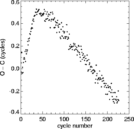
Figure 2: O–C diagram for run 3 relative to a test period of $6.774\,\Omega_{\rm b}^{-1}$. We take the dissipation rate ‘light curve’ from the outer disc ($r>0.2\,d$) and smooth it by taking a running mean over 200 points. The first ‘observed’ peak in the light curve occurred at $t=450.72\,\Omega_{\rm b}^{-1}$. The first forty or so cycles have mean period $6.905\pm 0.038\,\Omega_{\rm b}^{-1}$.

When the disc initially encounters the resonance, the oscillations induced in the simulation ‘light curve’ are of comparable magnitude to the background noise. There is thus considerable variation in the length of the first few cycles. Nevertheless it is apparent that the mean period of the first few cycles is less than the test period i.e. the first few cycles are shorter than the long term average period. Fig. 3, the O–C diagram of run 6 shows this clearly. The initial 25-30 cycles roughly form a concave upwards parabola indicating that $P_{\rm d}$ is increasing. Then $P_{\rm d}$ apparently decreases again to reach a stable value at about the same time that the eccentric instability saturates. Simulations where this is seen are marked in Table 1 with an $f$.

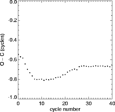
Figure 3: First 40 cycles of the O–C diagram for run 6 relative to a test period of $6.736\,\Omega_{\rm b}^{-1}$. We take the dissipation rate ‘light curve’ from the outer disc ($r>0.2\,d$) and smooth it by taking a running mean over 200 points. The first ‘observed’ peak in the light curve occurred at $t=155.50\,\Omega_{\rm b}^{-1}$.

The last four columns of Table 1 summarise the behaviour of the eccentric mode. As in Lubow (1991b)  and in Paper I, we determine the strength of the $(l\,\theta-m\,\Omega_{\rm b}t)$ mode, $S_{(l,m)}$, by Fourier decomposing the disc density distribution in azimuth and time. In particular we use $S_{(1,0)}$ to estimate the disc eccentricity. Column 8 gives a theoretical estimate for the exponential growth rate of the eccentricity in each disc. Column 9 lists the measured growth rate of $S_{(1,0)}$. Column 10 gives the strength of the eccentric mode at the end of each simulation. This value indicates how strongly the disc is affected by the resonance. The final column, which lists the time at which $S_{(1,0)}=0.01$, is a measure of when the disc initially encounters the resonance.

The theoretical estimates for the growth rate, $\lambda_{\rm t}$, are obtained using the analysis in Lubow (1991a). There, an expression was obtained for the eccentricity growth rate, $\lambda_{0}$, of a narrow ring of material at the resonance radius $r_{\rm res}$. The growth rate for a disc

$$\lambda_{\rm t}=C\lambda_{0},$$ (6)

where the correction factor

$$C=\frac{M_{\rm res}\,\,e_{\rm res}}{M_{\rm d}\,{<e>}}.$$ (7)

Here $M_{\rm res}$ is the mass of material in the resonance region, $M_{\rm d}$ is the total disc mass, $e_{\rm res}$ is the eccentricity at the resonance radius, and $<e>$ is the mass averaged eccentricity of the entire disc. We see from equation 7 that if there is sufficient mass at the resonance, and the eccentricity there is larger than the mass averaged value, it is possible for the eccentricity of a disc to grow at a faster rate than an ‘ideal’ narrow ring. We point this out as the rise times of superoutbursts are relatively short, which implies that the disc must become eccentric reasonably rapidly.

In calculating the values for $\lambda_{\rm t}$ in Table 1, and also in Paper I, we assumed that the eccentricity of the disc was uniform. Figure 4, a plot of $S_{(1,0)}$ at different radii as a function of time, shows that the eccentric mode strength in run 3 is an increasing function of the radius. We see from figure 5 that $S_{(1,0)}$ at the resonant radius is approximately three to five times the value for the entire disc. It is not unreasonable to assume the eccentricity behaved similarly in the other simulations (with the possible exception of run 2 where the resonance only weakly interacted with the disc). Therefore the values in column 8 may underestimate the ideal growth rate of the eccentricity by a factor five or so. This would make the disagreement between $\lambda_{\rm t}$ and $\lambda_{\rm m}$ more pronounced, with theory and simulation then only being in reasonable agreement for run 12. In all other cases the measured eccentricity growth is much slower than predicted by analysis.

SPH simulations by Lubow (1991b, 1992) that included only the $m=3$ component of the tidal potential (i.e. that component directly involved in the resonance), produced eccentricity growth rates that were in good agreement with the theory. However, when the full binary potential was used in the calculation, the eccentricity growth rate was much reduced. Lubow (1992) found that non-resonant stresses excited in the disc by the $m=2$ component of the tidal field were the principal culprits.

Figures 4 and 5 show the eccentricity growing equally rapidly at different radii. The time at which the mode strength reaches a plateau however, is a function of the radius. There is a huge inexplicable dip in the eccentric mode strength of the annulus $0.30\,d<r<0.35\,d$. In the absence of this trough, the mode appears to be growing at the same rate in this annulus as it is at other radii.

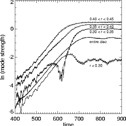
Figure 4: Logarithm of the eccentric mode strength $S_{(1,0)}$ as a function of time for various regions of the disc in run 3. Time units are $\Omega_{\rm b}^{-1}$.

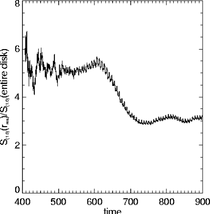
Figure 5: Ratio of the strength of the eccentric mode in the annulus $0.40\,d<r<0.45\,d$ to $S_{(1,0)}$ for the entire disc.

Figure 6: Each frame shows a few cycles of the light curve of one of the runs once the disc precession has fully developed. In each case we plot the rate of energy dissipation ($M\,d^{2}\,\Omega_{\rm b}^{3}$) at radii $r>0.05\,d$ as a function of time $(\Omega_{\rm b}^{-1})$. In runs 6 and 12 the disc has not reached a stationary state as the total mass (and the background dissipation rate) is still increasing. In all other cases the disc is in a ‘steady state’.

The periodic stressing of the disc as it rotates in the binary frame introduces a cyclic component into the simulation light curves, which we shall refer to as the ‘superhump signal’. The ‘superhumps’ from nine of the simulations are collected in Figure 6. The light curves produced by the low viscosity simulations (runs 6, 8 and 12 are illustrated) are clearly different from those of the high viscosity calculations. In the latter we see sharp spikes superposed on a lower amplitude, noisy signal which has two peaks per cycle. The low viscosity runs on the other hand have one tall reasonable broad peak per cycle, superposed on an almost flat background luminosity. The high frequency noise is much less apparent in these curves. We would also like to single out the light curve of simulation 2. Of all the high viscosity simulations it is the only one without the characteristic sharp spikes. The remaining superhump signal is of small amplitude and is almost swamped by high frequency noise. This is consistent with our interpretation that the disc in run 2 only barely encountered the resonance, and didn’t interact strongly with it.

In Paper I we showed that the sharp spikes in the high viscosity simulations were due to dissipation in small knots of material. These knots formed near apastron on highly eccentric orbits in the outer disc. The dissipation occurred when the knots, moving towards periastron, collided with gas on less eccentric orbits in the inner disc. These knotty structures are far less prominent in the low viscosity simulations. In general, the outer boundaries of the low viscosity discs are smoother and more regular than those of the high viscosity discs (see figures 8 and 12 of Paper I for density plots of runs 4 and 5), and the low viscosity discs have a less fragmentary appearance.

Recall from Paper I that the Shakura-Sunyaev viscosity parameter

$$\alpha(r)=\frac{1}{8}\,\zeta\,h\,\Omega(r)\,c^{-1},$$ (8)

where $\Omega(r)$ is the angular velocity at radius $r$ in the disc. Thus $\alpha(r_{\rm res})=3/16$ in simulations 7,8 and 12, $3/8$ in run 6, and $15/8$ in the other runs. The lower values are quite close to observational estimates of $\alpha$ for dwarf novae in superoutburst. This is pleasing because it is precisely these simulations that give results most similar to the observations.

In our simulations, the superhump signal is produced in the disc’s outer regions. In figure 7 we show approximately one superhump cycle from simulation 12, plotting the energy dissipated at radii $r>0.3\,d$ as a function of time. Compare the superhump’s amplitude of approximately $42\,\,M\,d^{2}\,\Omega_{\rm b}^{3}$ with the steady background luminosity at these radii of only $34\,\,M\,d^{2}\,\Omega_{\rm b}^{3}$ (keeping in mind that the disc is not in steady state). In figure 8 we show the locations of the particles responsible for the superhump signal. At each time shown we selected all the particles in the outer disc ($r>0.3\,d$) with a luminosity greater than a set threshold $(5.0\times 10^{-3}\,\,M\,d^{2}\,\Omega_{\rm b}^{3})$, and plotted them. The total luminosity of the selected particles is shown in the upper right corner of each frame. Matching these values to figure 7 it is clear that we have isolated the source of the hump in the simulation light curves.

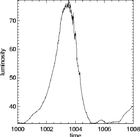
Figure 7: Luminosity, i.e. energy dissipation rate, ($M\,d^{2}\,\Omega_{\rm b}^{3}$) from radii $r>0.30\,d$ as a function of time ($\Omega_{\rm b}^{-1}$) for simulation 12.

Figure 8: The ‘superhump source’ for simulation 12. These nine plots, covering most of a disc rotation period $P_{\rm d}$, map the disc regions that are responsible for the signal shown in figure 7. In each frame, on axes corotating with the binary, we plot the ‘most luminous’ particles in the outer disc, i.e. those particles at radii $r>0.30\,d$ that have a luminosity greater than $5.0\times 10^{-3}M\,d^{2}\,\Omega_{\rm b}^{3}$. The total luminosity due to the selected particles is shown in the upper right of each frame, and the time is printed in the lower left. The x and y axes are scaled to the interstellar separation $d$. The Roche lobe of the primary is drawn in each frame. The system is rotating anticlockwise. The white dwarf primary is located at the origin.

4.2 Simulations of superoutburst

In this section we describe two simulations that test a key assumption of the thermal-tidal instability model; that tidal forces remove angular momentum more efficiently from a resonant disc than from a non-resonant disc. One can calculate the rate of angular momentum removal from a narrow gas ring at the $3:1$ resonance (see equation 62 of Lubow 1991a). But how efficiently can angular momentum be extracted from a disc that has just expanded into the resonance region at the beginning of a (normal) outburst? Is the resultant increase in energy dissipation large enough to account for observed superoutburst luminosities?

To simulate an outburst, we instantaneously increase the artificial viscosity in a simulation by a factor 5 or 10. This gives us only a crude approximation of an outburst, with the entire disc being suddenly forced to change from a cool, inviscid state to a hot, viscous state. A more detailed outburst model, that allows different parts of the disc to change state at different times could be easily implemented by allowing each SPH particle to have its own $\zeta$.

For the first calculation we subjected the low viscosity, $q=3/17$ disc (run 6) to a five-fold increase in viscosity, by setting $\zeta=10.0$ at time $t=100.00\,\Omega_{\rm b}^{-1}$. All other parameters were left unchanged. For reasons that will become clear shortly, we shall refer to this simulation as the ‘superoutburst calculation’. In the absence of any change in the viscosity, the run 6 disc encountered the resonance and became tidally unstable at $t_{\rm inst}=183.75$. However, with the aid of the sudden increase in the viscosity, the ‘superoutburst’ disc expanded and became resonant almost immediately.

The strongest non-resonant tidal response in the disc occurs in the $(2,2)$ mode. As such, the $(2,2)$ mode strength provides a measure of the radial extent of the disc. The relative strengths of the $(1,0)$ and $(2,2)$ modes also tell us whether the disc is resonant or non-resonant, or equivalently whether the disc is stationary in the inertial frame or stationary in the binary frame.

In figure 9, the $(1,0)$ and $(2,2)$ modes for the superoutburst calculation and for run 6 are plotted as functions of time. The sharp initial increase in the $(2,2)$ mode strength shows that the superoutburst disc rapidly expanded in response to the increase in viscosity. However, tidal instability then set in. As the disc eccentricity rose, tidal torques became more efficient at removing angular momentum from the disc. Consequently the disc shrank once more, as witnessed by the subsequent decline in the $(2,2)$ mode. The weakening of the $(2,2)$ mode implied an increase in the inward mass flux $\dot{M}_{\rm d}$ which, as we shall see below, caused an increase in the disc luminosity.

Tidal instability also caused the disc in run 6 to shrink, but much less dramatically. Note that the eccentricity in run 6 continued increasing even after the tidal instability had became saturated at $t=300\,\Omega_{\rm b}^{-1}$. In this case, both the total disc mass and angular momentum continued to grow because tidal torques were still not strong enough to remove all the angular momentum being added with new disc material at $r_{\rm c}$.

Light curves for run 6 and the superoutburst simulation are plotted in figure 10. Note that the superoutburst disc was initially much more luminous than the disc in run 6. However the excess luminosity decayed fairly rapidly. Recall that the inwards mass flux in an axisymmetric, Keplerian disc is given by

$$\dot{M}_{\rm d}=6\pi r^{\frac{1}{2}}\frac{{\rm\partial}}{{\rm\partial}r}(\nu\Sigma r^{\frac{1}{2}}).$$ (9)

From equation 9 it is apparent that the instantaneous viscosity increase caused $\dot{M}_{\rm d}$ to increase to a rate greater than the mass transfer rate from the secondary. This lead to a general decline in density in the disc, which in turn caused $\dot{M}_{\rm d}$ to decay to a steady state value. Thus the initial decline in the superoutburst disc luminosity is explained.

But the luminosity of the superoutburst simulation did not then flatten out. Rather, it reached a minimum value of $707.46\,M\,d^{2}\,\Omega_{\rm b}^{3}$ at $t=148.92\,\Omega_{\rm b}^{-1}$ and then rose once more. The minimum in the luminosity coincided almost exactly with the maximum strength of the $(2,2)$ mode which occurred at $t=141.83\,\Omega_{\rm b}^{-1}$. The mean luminosity in the superoutburst simulation peaked at about $1000\,M\,d^{2}\,\Omega_{\rm b}^{3}$ at time $t=240\,\Omega_{\rm b}^{-1}$. Thus there was a 40–50 % increase in the energy output of the disc over a time interval of about 15 orbital periods. In other words the disc brightened by about 0.4 magnitudes over approximately one day, which is consistent with observations of the rise to superoutburst maximum.

The disc luminosity then slowly declined as the disc adjusted to the increased tidal torques at the outer edge. The light curve is qualitatively similar to the extended decline of a superoutburst. The limitations of our simulation probably preclude closer comparison with observations. For a start we used an isothermal equation of state (i.e. the speed of sound was constant). The effective Shakura-Sunyaev viscosity parameters of our simulations were much larger than those found by Cannizzo (1993b) to be appropriate for a normal outburst. For the superoutburst simulation we had $\alpha_{\rm hot}(r_{\rm res})=15/8$ and $\alpha_{\rm cold}(r_{\rm res})=3/8$. Also, the ratio $\alpha_{\rm hot}/\alpha_{\rm cold}=5$ in our simulation, which was rather small. Furthermore, rather than having a constant $\alpha$ throughout, our simulations have constant kinematic viscosity $\nu$. One would expect that the proportion of the disc mass that enters the resonance region, and hence the superoutburst luminosity will be dependent upon $\nu$.

Note also in figure 10 that the superhump signal appeared well before the ‘superoutburst maximum’. Superhumps are not usually observed until approximately a day after superoutburst maximum has occurred. However, recent observations of both ER UMa (Kato, Nogami & Masuda 1996) and V1159 Orionis (Patterson et al. 1995) found superhumps on the rise to superoutburst maximum.

Some idea of the radial dependence of the superoutburst luminosity can be gained from figure 11, in which light curves generated by different annuli of the superoutburst disc are plotted. The initial luminosity dip up to time $t\simeq 200\,\Omega_{\rm b}^{-1}$ was shallower at larger radii. Indeed, at the largest radii (not shown) the dip was in fact a hump, reflecting the initial expansion of the disc in response to the increase in $\zeta$. Figure 11 shows that the superoutburst in the inner disc is delayed somewhat with respect to the superoutburst in the outer regions. This is consistent with there being an enhancement in the mass flux at the outer edge of the disc which then works its way inwards. As a result the superoutburst light became somewhat bluer with time. Also notice that the superhump signal first became apparent, and had the largest amplitude, in the light curve of the annulus $0.20\,d<r<0.30\,d$. A small superhump signal appeared somewhat later in the $0.10\,d<r<0.20\,d$ light curve.

We completed a second ‘normal outburst’ calculation, using run 12 ($q=1/19$, $\zeta=1.00$) as the seed simulation. At $t=300.00\,\Omega_{\rm b}^{-1}$ we reset the viscosity to $\zeta=10.0$, but left the other parameters unchanged. The $(1,0)$ and $(2,2)$ mode strengths for the normal outburst simulation and run 12 are plotted as functions of time in figure 12. Shortly after $t=300.00\,\Omega_{\rm b}^{-1}$ the radial expansion of the run 12 disc was arrested as the disc became unstable ($t_{\rm inst}=342.19$). However at mass ratio $q=1/19$ the $3:1$ resonance is too weak to drive a disc with $\zeta=10.0$ to tidal instability (see run 11). Hence, in the normal outburst simulation, the sudden increase in $\zeta$ simply caused the disc to expand radially. The eccentricity in the normal outburst simulation did not increase.

Light curves for run 12 and the normal outburst simulation are shown in figure 13. The normal outburst simulation luminosity declined rapidly from a high initial value as the disc adjusted to the increased viscosity. This time however, without a tidal instability sponsored increase in the mass flux, there was no second rise in the luminosity. The diminutive superhumps of run 12 clearly show how weak the $3:1$ resonance is for this mass ratio.

The simulations described in this section provide support for the thermal-tidal instability model for superoutburst. In particular, we find that when a rapidly expanding disc encounters the $3:1$ eccentric inner Lindblad resonance and becomes tidally unstable, large quantities of angular momentum are removed from the disc causing it to shrink once more. The energy released is sufficient to account for the excess luminosity of a superoutburst.

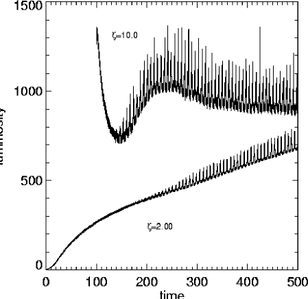
Figure 10: Luminosity $(M\,d^{2}\,\Omega_{\rm b}^{3})$ from radii $r>0.05\,d$ in the superoutburst simulation. The equivalent light curve for run 6 is also plotted (lower curve). Note that a superhump signal is apparent in both curves.

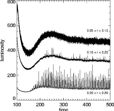
Figure 11: Luminosity $(M\,d^{2}\,\Omega_{\rm b}^{3})$ of various disc annuli in the superoutburst simulation. Notice that the superhump signal predominately comes from radii $r>0.20\,d$. From bottom to top, the curves have minima at $t=137.37$,$143.03$ and $154.58\,\,\Omega_{\rm b}^{-1}$.

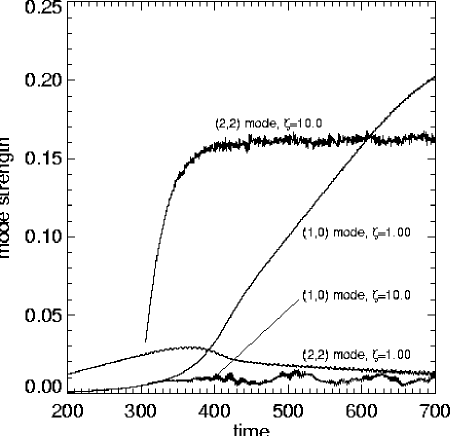
Figure 12: Mode strengths for the normal outburst simulation ($\zeta=10.0$), and for run 12 ($\zeta=1.00$). Time (in $\Omega_{\rm b}^{-1}$) is measured from the beginning of run 12. Thus the normal outburst simulation starts at $t=300.00\,\Omega_{\rm b}^{-1}$.

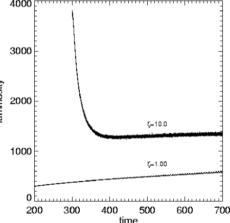
Figure 13: Luminosity $(M\,d^{2}\,\Omega_{\rm b}^{3})$ from radii $r>0.05\,d$ in the normal outburst simulation. The equivalent light curve for run 12, is also plotted (lower curve). Note that a superhump signal is only apparent for run 12.

5 Conclusions

We conclude that the disc precession period (which we identify with the superhump period) is not uniquely determined by the binary mass ratio. This point is clearly illustrated by figure 14, where the ‘superhump period excesses‘, $(P_{\rm d}-P_{\rm b})/P_{\rm b}$, for the simulations of section 4.1 are plotted against $q$. We find that gas pressure and viscosity are also important in determining the disc precession period. This conclusion contradicts the findings of Whitehurst & King (1991). Concluding that the binary mass ratio was the sole factor that determined the precession period, they estimated $P_{\rm d}$ from the orbital periods of non-interacting test particles moving in the binary’s gravitational potential. Specifically, they estimated that the superhump period was equal to the period of doubly periodic test particle orbits in the vicinity of the resonance, as measured in the inertial frame. Setting to one side for a moment concerns about using non-interacting particles, in the observations and in the simulations, the superhump phenomenon recurs at a common position in the binary frame. Hence their estimate should have been

$$P_{\rm d}\simeq P_{\rm b}(1+w/\Omega_{\rm b})$$ (10)

where $\omega$ is the angular rate of precession of the particle’s line of apsides.

We do not wish to overstate the case as figure 14 clearly shows the superhump period excess increasing with mass ratio, indicating that the tidal potential is most important in the determination of $P_{\rm sh}$. However, if we are to use an expression similar to equation 10 to predict the binary mass ratio from the orbital and superhump periods, then viscosity and gas pressure must be accounted for. We mentioned in section 4.1 that increasing the gas pressure had a retrograde effect upon the disc precession. Such an effect may be significant in actual SU UMa systems. Recall that equation 2, the empirical relationship between the superhump and binary periods, suggests that systems with very small orbital period (and hence by inference a very small mass ratio) will have $P_{\rm sh}<P_{\rm b}$. We suggest that this is due to gas pressure slowing the disc precession in the manner described in Lubow (1992).

We found small but significant changes in the disc precession period. In several cases, $P_{\rm d}$ decreased slightly once the resonance had saturated and the disc eccentricity had stabilised. Thus it may be possible to use the small changes in $P_{\rm sh}$ over the course of a single superoutburst to determine whether disc eccentricity is growing or declining.

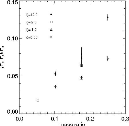
Figure 14: Superhump period excess (with error bars shown) as a function of binary mass ratio for the simulations of section 4.1.

Both in Paper I and here (see figure 8) we showed where in the disc the periodic component of the thermal energy generation occurs. However, we neglected the details of the disc’s vertical structure in our calculations, and so we must be very cautious about comparing these results with observational attempts to isolate the superhump source (e.g. Warner & O’Donoghue 1988, and O’Donoghue 1990). In other words, the time taken for energy released on the disc midplane to reach the disc surface is likely of the order of a dynamical time (${\Omega(r)}^{-1}$).

Billington et al. (1996) found dips in the ultraviolet light from the inner disc of OY Car in superoutburst that coincided with the superhumps. Using a modified eclipse mapping technique, they showed that the dips could be explained if the disc had a raised outer rim that obscured the inner disc. Figures 7 and 8 showed that in simulation 12 the ‘superhump source’ accounted for just over half the outer disc luminosity. This indicates that there are sufficiently large azimuthal temperature gradients in the outer disc to generate the 10-20% variations in the height of the outer disc that the observations of Billington et al. imply. They suggest that the superhump luminosity is actually ultraviolet radiation from the inner disc that is reprocessed down to the optical in the raised disc rim. In our simulations, the periodic component of the ‘light curve’ was of sufficient amplitude to be comparable to superhumps. We propose that the original superhumps are powered simply by the variable thermal energy dissipation in the outer disc. This would naturally generate an outer disc that varied in height with azimuth. It is possible that reprocessing of light from the inner disc causes further evolution in the disc rim, leading to the late superhumps that are seen towards the end of a superoutburst.

Whitehurst & King concluded that the growth rate of the tidal instability was too slow to be consistent with observations of superoutbursts. They suggested that a burst of mass transfer from the secondary was required to accelerate the rate at which the disc becomes eccentric. We do not agree with that conclusion. Our results show that a disc can become eccentric on a time scale consistent with the rise time of a superoutburst. Recall that in figure 11 superhump-like modulations of the light curve were visible on the rise to maximum luminosity. In this simulation mass was added in circular orbit at radius $r_{\rm c}$. We found that mass addition from $L_{1}$ slowed rather than accelerated growth in the $(1,0)$ mode (not however to a rate that was inconsistent with superoutburst observations). Lubow (1994)  found analytically that the impact of the stream upon the disc acted to reduce disc eccentricity.

Finally, the simulations of section 4.2 provide strong support for the thermal-tidal instability model for superoutburst. We approximated a dwarf nova outburst by instantaneously increasing the shear viscosity. We found that when a rapidly expanding disc also became tidally unstable, there was an increase in the disc luminosity that was consistent with a superoutburst. In our simulation, superhump-like modulations were apparent on the rise to maximum luminosity. In a second case, where the expanding disc did not become tidally unstable, there was no increase in the luminosity.

The author would like to thank Steve Lubow for much encouragement, useful advice and constructive criticism.

References

- [1] Billington, I., Marsh, T. R., Horne, K., Cheng, F. H., Thomas, G., Bruch, A., O’Donoghue, D., Eracleous, M., 1996, 279, 1274
- [2] Cannizzo, J.K., 1993a, in Wheeler J. C., ed., Accretion Disks in Compact Stellar Systems, World Scientific, Singapore, p. 6
- [3] Cannizzo, J.K., 1993b, ApJ, 419, 318
- [4] Flebbe, O., Münzel, S., Herold, H., Riffert, H., Ruder, H., 1994, ApJ, 431, 754
- [5] Hirose M., Osaki Y., 1990, PASJ, 42, 135
- [6] Kato, T, Nogami, D., Masuda, S., 1996, PASJ, 48, L5
- [7] Lin D. N. C., Pringle J. E., 1976, in Eggleton P., ed., Structure and Evolution of Close Binary Systems. D Reidel, Dordrecht, p. 237
- [8] Lubow S. H., 1991a, ApJ, 381, 259
- [9] Lubow S. H., 1991b, ApJ, 381, 268
- [10] Lubow S. H., 1992, ApJ, 401, 317
- [11] Lubow S. H., 1994, ApJ, 432, 224
- [12] Lubow S. H., Shu F. H., 1975, ApJ, 198, 383
- [13] Murray, J. R., 1996, MNRAS, 279, 402
- [14] O’Donoghue D., 1990, MNRAS, 246, 29
- [15] Osaki, Y., 1989, PASJ, 41, 1005
- [16] Osaki, Y., 1996, PASP, 108, 39
- [17] Paczyński, B., 1977, ApJ, 216, 822
- [18] Papaloizou, J., Pringle, J., E., 1977, MNRAS, 181, 441
- [19] Patterson, J., Richman, H., 1991, PASP, 103, 735
- [20] Patterson, J., Jablonski, F., Koen, C., O’Donoghue, D., Skillman, D. R., 1995, PASP, 107, 1183
- [21] Retter, A., Leibowitz, E. M., Ofek, E. O., 1997, to appear in MNRAS
- [22] Thorstensen, J. R., Patterson, J. O., Shambrook, A., Thomas G., 1996, PASP, 108, 73
- [23] Warner, B., 1995, Cataclysmic Variable Stars. Cambridge University Press, Cambridge
- [24] Warner, B., O’Donoghue, D., MNRAS, 1988, 233, 705
- [25] Watkins, S. J., Bhattal, A. S., Francis, N., Turner, J.A., Whitworth, A. P., 1996, A&AS, 119, 177
- [26] Whitehurst, R., 1988, MNRAS, 232, 35
- [27] Whitehurst, R., 1994, MNRAS, 266, 35
- [28] Whitehurst, R., King, A., 1991, MNRAS, 249, 25