Microlensing of Globular Clusters as a Probe of Galactic Structure

Abstract

The spatial distribution of compact dark matter in our Galaxy can be determined in a few years of monitoring Galactic globular clusters for microlensing. Globular clusters are the only dense fields of stars distributed throughout the three-dimensional halo and hence are uniquely suited to probe its structure. The microlensing optical depths towards different clusters have varying contributions from the thin disk, thick disk, bulge, and halo of the Galaxy. Although measuring individual optical depths to all the clusters is a daunting task, we show that interesting Galactic structure information can be extracted with as few as $40$–$120$ events in total for the entire globular cluster system (observable with 2–5 years of monitoring). The globular cluster microlensing is particularly sensitive to the core radius of the halo mass distribution and to the scale length, surface mass density, and radial scale height variations of the thin disk.

1 Introduction

The search for compact dark matter in the mass range $10^{-6}$–$10^{2}{\,M_{\odot}}$ using microlensing (Paczyński 1986) has come to fruition with the detection of many microlensing events towards the Galactic bulge, Large Magellanic Cloud, and Small Magellanic Cloud by various projects to monitor millions of stars (Alcock et al. 1993, 1996, 1997a,b; Aubourg et al. 1993; Udalski et al. 1993). These studies have confirmed the presence of a massive bar in the Galaxy by detecting more microlensing events than expected towards the Galactic bulge (Udalski et al. 1994; Alcock et al. 1995a; Paczyński et al. 1994; Zhao, Spergel, & Rich 1995) and have found evidence for a massive halo by detecting 8 times more events towards the Large Magellanic Cloud (LMC) than can be explained by known stellar populations (Alcock et al. 1997a).

Uncertainties in the spatial distribution, kinematics, and masses of the lensing objects remain (cf. review by Paczyński 1997). One of the major uncertainties is our incomplete knowledge of Galactic structure. Possible locations for the lenses include a maximal Galactic disk (Kuijken 1997), the LMC’s disk (Sahu 1994), and the Galaxy’s halo. Here we propose using globular cluster stars as background objects to discriminate the spatial distribution of the lensing objects statistically. This is possible because the globular clusters are distributed throughout the halo of our Galaxy, albeit concentrated towards the center. Therefore we can probe many lines of sight through varying amounts of the halo, disk, and bar of the Galaxy to determine the relative contributions of each to microlensing. Similar strategies using the ratios of Bulge, LMC and SMC optical depths have been suggested by Sackett and Gould (1993) to constrain halo flattening, and by Gould, Miralda-Escudé & Bahcall (1994) to constrain relative contributions of the thin and thick disks and the halo.

Another concern for microlensing studies is that the Galactic halo may be clumpy, as would be expected under the Searle and Zinn (1978) picture of Galaxy formation. The discoveries of the Sagittarius dwarf galaxy (Ibata, Gilmore & Irwin 1994) and of a possible intervening population towards the LMC (Zaritsky & Lin 1997) provide examples of clumps of stars, in tidal tails or dwarf spheroids in the halo, that might raise the number of microlensing events towards some lines of sight (Zhao 1997). Monitoring microlensing events towards many Galactic directions where globular clusters are located will average over such fluctuations in halo density and thereby alleviate the potential worry about non-representative lines of sight.

Because the globular clusters are distributed throughout the Galaxy’s halo, such a campaign of monitoring along different Galactic directions would be invaluable for weighing the compact massive component of the Galaxy (in stars or brown dwarfs) not only in the halo, but also in the thick disk, thin disk, and bulge. Measuring individual optical depths to the clusters is not practical, but interesting Galactic structure information can be extracted with as few as $40$–$120$ events in total for the entire globular cluster system (observable with 2–5 years of monitoring).

In section 2, we review necessary background information on microlensing and on the globular clusters. We take M 15 as an example and discuss the observability of lensing events in globular clusters, using resolved stars and pixel lensing. In section 3, we study the number of events required to distinguish between representative Galaxy models using Monte Carlo simulations. Finally, in section 4 we discuss some more implications of this work and summarize our conclusions. An appendix contains analytic results that supplement the simulations in section 3.

2 Microlensing of a Globular cluster

The optical depth to microlensing is defined as the probability that a background source will be amplified by a factor $1.34$ (Refsdal 1964; Vietri & Ostriker 1983). This amplification corresponds to the background source lying inside the Einstein radius of the lens. Because the area in the Einstein ring is proportional to lens mass, the optical depth depends only on the mean mass density and not on the masses of individual lensing objects, provided only that the Einstein radius substantially exceeds the physical size of both source and lens. This condition requires lensing masses $M\gtrsim 10^{27}\hbox{g}\sim M_{\oplus}$ for length scales typical in the Galaxy. The geometry of source, lens, and observer affect the Einstein radius, and the full expression for the lensing optical depth $\tau$ is (Vietri & Ostriker 1983)

$$\tau=\int_{0}^{D}{4\pi G\rho\over c^{2}}L\left(1-{L\over D}\right)dL$$ (1)

where $D$ is the distance to the background source, $L$ is the distance along the line of sight, $\rho$ is the local mass density at distance $L$, and $G$ and $c$ are the gravitational constant and the speed of light.

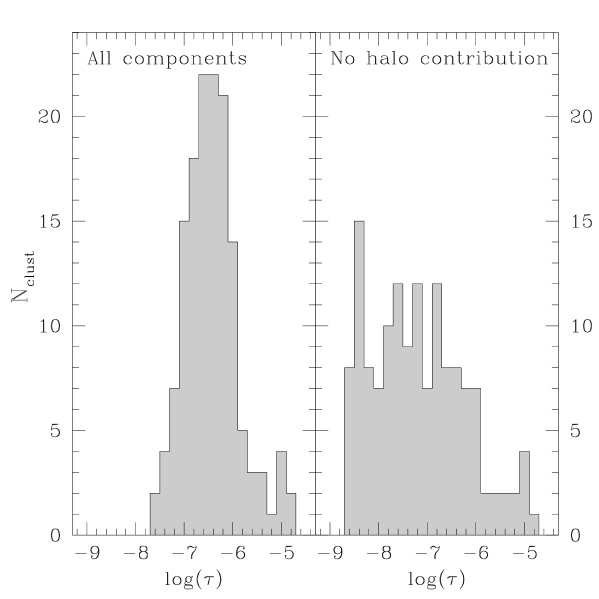
Figure 1: Histograms of microlensing optical depths to Galactic globular clusters under a “standard” model (model 5,6,7a in table 1). Left panel: Histogram of total optical depths. Right panel: Histogram of the optical depth due to the disk and bar components alone. The latter case is a lower bound to the expected optical depths, and omits the lensing contribution of both the stellar halo and the dark matter halo.

The Galaxy has $\sim 150$ globular clusters, distributed in a spheroidal halo about the Galactic center. Each typically contains $\sim 10^{4}$–$10^{5}$ stars to a limiting magnitude of $V\leq 22$, giving a total of $\simeq 10^{6}$–$10^{7}$ stars to monitor. The optical depth to the clusters is $10^{-6}$–$10^{-8}$, depending on the cluster location in the Galaxy and the Galactic model (Figure 1). In addition to the lensing optical depth, a full analysis would need to consider the mass distribution of the lenses and their velocities in order to predict the event rate and duration. These can then be compared to the time sampling of monitoring projects to determine the efficiency of a search. Such exhaustive analyses have been carried out for the Galactic bulge, Magellanic clouds, and M31 (Alcock et al 1995b), which are already being monitored. Observationally, the median duration of events towards the bulge is 30 days (Alcock et al 1997a). The typical timescale for globular cluster microlensing events may be comparable or somewhat different, depending on the relative kinematics of globular clusters and the lensing populations.

The number of stars in a globular cluster that can be resolved and individually monitored from the ground will depend upon the number of stars in the cluster, the degree of concentration, the distance to the cluster and the seeing conditions. In the inner regions, crowding (up to 130 stars per square arcsecond for $V<22$) is too severe for individual stars to be observed. Here one can instead monitor the brightness variations of pixels, which are a combination of many stars; this is the so-called pixel-lensing regime (Crotts 1992; Colley 1995).

We account for crowding by first calculating the effective number of stars that can be monitored in the cluster M 15, and then scaling the results for clusters of other luminosities and heliocentric distances. We chose M 15 as an example because stars in the interior core (down to $0.3\arcsec$) have been resolved by Hubble Space Telescope observations (Guhathakurta et al. 1996). M 15 is at a distance of $\simeq 10\,\hbox{kpc}$, about the median distance to globular clusters. It has a high concentration index, which will lead us to a conservative (low) estimate for the fraction of resolved stars in a typical cluster. M 15 is also 2.7 times brighter (in V-band absolute flux) than the average cluster.

The stars in the crowded interiors of Globular clusters can be monitored for pixel lensing events, where one pixel brightens due to the microlensing of one of the unresolved stars. The rate of detectable lensing events for each star is lower than in the uncrowded regime, because for a fixed amplification of the total flux in a pixel, a star needs to undergo a larger magnification, which depends on the fraction of light in the pixel arising from that star. This in turn depends on the number of stars in the pixel and the brightness of the star. Since the crowding varies continuously, decreasing from the unresolved core to resolved stars in the exterior, we calculate the mean effective optical depth for the entire cluster using a pixel microlensing formalism. In the outer regions of the cluster, where the surface density drops to $\lesssim 1$ star per pixel, the lensing cross sections approach the typical Einstein ring area.

Suppose a microlensing event is claimed for a fixed fractional increase in the brightness of a pixel. Following Colley (1995),

$$\Delta m=-2.5\times\log{{Aqf_{*}+f_{pix}}\over{qf_{*}+f_{pix}}}~{}~{},$$ (2)

where $\Delta m$ is the brightness change in magnitudes, $A$ is the amplification, $q$ is the fraction of the amplified star’s light falling in the peak pixel of the point spread function, $f_{*}$ is the flux of the star, and $f_{pix}$ is the flux due to other sources in the pixel. The maximum radius $u$ that produces amplification $A$ is given by (Refsdal 1964)

$$A={{u^{2}+2}\over{u\sqrt{u^{2}+4}}}$$ (3)

where $u=R/R_{E}$, and $u^{2}$ gives the area as a fraction of the area of the Einstein ring area $\pi R_{E}^{2}$. If the star were resolved and the only one contributing to the flux in that pixel, $u=1$ and $A=3/\sqrt{5}$. Using the luminosity function of M 15 and its surface brightness profile (Guhathakurta et al 1996; Trager, King, & Djorgovski 1995) we calculate the loss of efficiency, which is the ratio of the area in the lens plane required to brighten the star in a field of surface brightness $S$ vs when it is alone. This is a function of the surface brightness of the pixel and the brightness of the star. Summing over the stellar luminosity function $f(m)$ for M 15 (Guhathakurta 1996) in V band,

$${\cal E}(r)=\left.\int_{m_{1}=12}^{m_{2}=22}f(m)u(m)^{2}dm\right/\int_{m_{1}=12}^{m_{2}=22}f(m)dm~{}~{},$$ (4)

where $u$ has an implicit dependence on the local surface brightness and hence on $r$. The value of ${\cal E}$ varies from $6.4\times 10^{-4}$ at a radial distance of $0.1\arcsec$ from the center and approaches 1 at $r\simeq 500\arcsec$ when stellar density reaches 0.12 stars per square arcsecond. With $3\times 10^{5}$ stars to a radius of $600\arcsec$ and a mean efficiency of $\langle{\cal E}\rangle=65.9\%$, the cluster can be treated like a cluster with $2\times 10^{5}$ fully resolved stars.

For other globular clusters, we retained the radial profile and luminosity function models from M 15. The total numbers of stars were scaled relative to M 15 according to each cluster’s V band luminosity. The projected distribution on the sky (and hence crowding) and the number of stars above our $V<22$ cutoff were adjusted for the distances to the individual clusters. The mean number of effectively resolved stars inside a $600\arcsec$ radius was $5.7\times 10^{4}$ per cluster.

3 Distinguishing between Galactic models

We report here on a series of simulations to determine how well microlensing observations of globular clusters can distinguish among plausible Galactic models. In each test, the microlensing optical depth towards each cluster is calculated under two assumed Galactic models, and the probability of inferring the correct model is calculated for a given number of events. The results are then inverted to calculate the number of microlensing events needed to infer the correct Galactic model from the distribution of lensing events among the clusters with 90% confidence.

The models generally consisted of three mass components: The thin disk, the halo, and the central bar. A fourth component, the thick disk, was added in one model. All the mass is assumed to be in compact objects. The optical depth to microlensing is calculated using equation (1), substituting the density $\rho=\rho_{\hbox{disk}}+\rho_{\hbox{bar}}+\rho_{\hbox{halo}}+\rho_{\hbox{thick disk}}$.

The models were required to obey three constraints. (1) Rotation Curve: The potential of the Galaxy consisting of these components was required to fit the rotation curve in the inner Galaxy excluding the bar region ($2.5\,\hbox{kpc}<R<R_{0}$) and a flat rotation curve with circular speed $220\,\hbox{km}/\hbox{s}$ in the outer Galaxy ($R_{0}<R<16.5\,\hbox{kpc}$) (Knapp, Tremaine, & Gunn 1978; Gunn, Knapp, & Tremaine 1979; Fich, Blitz, & Stark 1989; Malhotra 1994, 1995). $R_{0}$ is the Sun-Galactic Center distance, and is taken to be $8.5\,\hbox{kpc}$ throughout this work. (2) The second constraint is the local surface mass density of the thin disk, $\Sigma_{0}$, which lies in the interval $40M_{\odot}/\,\hbox{pc}^{2}\lesssim\Sigma_{0}\lesssim 80M_{\odot}/\,\hbox{pc}^{2}$ (Kuijken & Gilmore 1989, 1991; Bahcall, Flynn, & Gould 1992; Flynn & Fuchs 1994). We implement this by either fixing the local surface mass density or adjusting other parameters to ensure that the final value lies in the observationally acceptable range. This resolves some of the degeneracy between the radial force due to the disk and that due to the halo. (3) A third, implicit, constraint is the mass profile of the thin disk. From gas dynamics it is demonstrated to be an exponential with roughly the same scale length as the light (Knapp 1990; Malhotra 1995, 1994).

The Thin Disk: The functional form of the disk density component(s) was taken to be

$$\rho_{d}=\Sigma_{0}/(2z_{1})\times\exp(-[r-R_{0}]/r_{1})\times(\hbox{sech}[z/z_{1}])^{2}~{}~{},$$ (5)

where $r_{1}$ is the exponential scale length, $z_{1}$ is the scale height, and $(r,z)$ are Galactocentric cylindrical coordinates (Spitzer 1942). We took $z_{1}=0.20\,\hbox{kpc}$ at the Solar radius. The scale height was usually kept constant with radius. Such constancy is indicated by most studies of external galaxies (van der Kruit & Searle 1982), and is consistent with the diffuse near infrared light of the Milky Way (Spergel, Malhotra, & Blitz 1996; Freudenreich 1996). However, there may be exceptions to this rule (de Grijs & Peletier 1997), so in one case [model 5B] the scale height was allowed to increase with radius according to $z_{1}\propto 1/\Sigma(r)\propto\exp(r/r_{1})$. This flaring is the appropriate behavior for a self-consistent isothermal thin disk with constant vertical velocity dispersion and exponentially decreasing surface density.

Halo: A power law halo was adopted, following Evans (1993,1994) and Alcock et al (1995b):

$$\rho_{h}={v_{0}^{2}\over 4\pi Gq^{2}}{(1+2q^{2})r_{c}^{2}+r^{2}+(2-q^{-2})z^{2}\over\left(r_{c}^{2}+r^{2}+z^{2}/q^{2}\right)^{2}}~{}~{},$$ (6)

where $r_{c}$ is the core radius of the halo and $q$ the halo flattening parameter. Note that Alcock et al’s parameter $\beta$ has been set to $\beta\equiv 0$, so that the asymptotic behavior at large radii is a flat rotation curve with circular speed $v_{0}$. The power law halo component admits a self-consistent distribution function and an analytic potential; the latter was useful in ensuring that the models match observational rotation curve constraints. We do not include halo truncation, since relatively few globular clusters lie at galactocentric radii $\gg 10\,\hbox{kpc}$ while present evidence suggests the halo extends to $40$–$50\,\hbox{kpc}$ (Little & Tremaine 1987).

Bar/Bulge: Detailed models of the central bar of our Galaxy have now been constructed by several groups (Dwek et al 1995; Zhao et al 1995; Stanek et al 1997). We chose to follow the Zhao et al (1995) bar model:

$$\rho_{b}={M_{b}\over 8\pi abc}e^{-s^{2}/2}$$ (7)

where $a=1.49\,\hbox{kpc}$, $b=0.58\,\hbox{kpc}$, and $c=0.40\,\hbox{kpc}$ are the major axis, minor axis, and vertical scale lengths; $s^{4}=\left[(x/a)^{2}+(y/b)^{2}\right]^{2}+(z/c)^{4}$; and $(x,y,z)$ is a Cartesian coordinate system aligned with the bar. We took the major axis of the bar to be at an angle $\phi$ with respect to the Sun-Galactic center line, and took the plane $z=0$ to be the Galactic plane (so that the bar is not tilted). In the rotation curve fits, we did not include data closer than $2.5\,\hbox{kpc}$ from the Galactic center, because of complex non-circular motions in the bar, and approximated the potential of the bar as a point source potential of the same mass.

Tests: Seven tests were executed in all. Each determined the sensitivity of globular cluster microlensing observations to one parameter by comparing two paired models having a range of that parameter. Other structural parameters were adjusted as needed to maintain consistency with the rotation curve. The models are summarized in table 1. Test 1 is designed to discriminate between models with a large and small halo core radius. Other components necessarily become more massive in the case of a large core radius. Test 2 varies the halo flattening parameter, while keeping everything else fixed. Test 3 uses a fixed disk mass but a range of disk scale length; the halo parameters here change substantially also. Test 4 primarily explores local disk surface mass density. Test 5 allows the scale height of the thin disk to increase with Galactocentric radius. Test 6 includes a thick disk component of scale height $600\,\hbox{pc}$, surface density $1M_{\odot}/\,\hbox{pc}^{2}$, and scale length identical to the thin disk. Finally, test 7 varies the angle of the Galactic bar with respect to the Sun-Galactic center line. Note that the rotation curve constraint couples the parameters of different Galactic components in our models. Differences between microlensing optical depths in models A and B of a test may thus be due to changes in more than one Galactic component.

For each model, the microlensing optical depth to each cluster was determined by evaluating equation (1) numerically for the density model given by equations (5)–(7). Our cluster sample consisted of 140 globular clusters whose coordinates, distances, and absolute V band magnitudes are tabulated in Djorgovski & Meylan (1993) and Djorgovski (1993). As a consistency check, we also implemented some of the halo models by Sackett & Gould (1993), and verified that our numerical integration code reproduced their optical depths towards the Magellanic Clouds and Galactic Bulge within 1%.

Given the optical depths, we then approximated the effect of an observing campaign by defining the effective number $n$ of trials per star monitored. This is essentially the number of independent lensing events we expect to observe per unit optical depth, or equivalently, the number of event durations spanned by the observing campaign. Formally, $n$ is defined by $\langle E_{*}\rangle=n\tau$, where $\langle E_{*}\rangle$ is the number of events expected per star monitored and $\tau$ is the lensing optical depth. Accounting for inefficiencies in the monitoring program, we write $n\approx\epsilon t/d$. Here $t$ is the duration of the monitoring program, $d$ is the mean duration of lensing events, and $\epsilon$ is the fraction of events that will be detected given the time sampling of the observing program. The observing efficiency $\epsilon$ can be approximated as $\epsilon=\epsilon_{1}\epsilon_{2}$, where $\epsilon_{1}$ is the fraction of the year a source can be monitored and $\epsilon_{2}$ is the fraction of events with durations longer than the time between observations and shorter than $t$. Note, though, that a precise calculation of $n$ would require the full 6-dimensional phase space distribution function of the lenses to determine $\epsilon$. We use the approximations $d\sim 30\,\hbox{days}$ and $\epsilon\sim 0.3$, so that $n\sim 3.5\times(t/\hbox{yr})$.

A simulation consists of assuming a uniform number of trials $n$ for all clusters, and for each cluster drawing a random number of “observed” events from a Poisson distribution with mean $\langle E\rangle=N_{*}n\tau$ under an assumed Galaxy model. The likelihood of obtaining the resulting fake data set is then computed under this model and under an alternate model. The model with the larger likelihood is taken as the inferred model. Many such simulations are run to obtain the probability of inferring the wrong model for each assumed model / alternate model pair. The test is then repeated for many values of $n$. In the limit of infinite data ($n\rightarrow\infty$), the probability of error goes to zero.

Table 1 contains values of the effective number of trials $n_{90}$ required to distinguish between the two models in each test at the 90% confidence limit (i.e., with a 10% chance of inferring the incorrect model). Because this probability need not be the same for the two input models, two values of $n_{90}$ are tabulated for each test. To determine $n_{90}$, we interpolate between measured error probabilities in simulations at a few values of $n$ using scaling relations from appendix A: $p(\hbox{error})=\hbox{erfc}(h)/2$ where $h\propto\sqrt{n}$. These scaling relations can also be used to determine the values of $n$ needed to achieve other confidence levels in distinguishing between models.

Model	$\Sigma_{0}$	$r_{1}$	$v_{0}$	$r_{c}$	$q$	$M_{b}$	$\phi$	$\log_{10}[n_{90}]$	$E_{tot,90}$
1A	40	3.5	175	2.5	0.8	1.00	25	0.82	51.3
1B	50	3.0	201	10.0	0.8	1.31	25	0.78	42.5
2A	50	3.0	183	6.9	1.0	1.00	25	1.60	263
2B	50	3.0	183	6.9	0.625	1.00	25	1.63	315
3A	67	3.5	161	5.43	0.8	1.00	25	1.10	89.9
3B	50	2.5	220	16.15	0.8	1.00	25	1.06	80.6
4A	80	3.31	200	15.21	0.8	1.00	25	1.19	110
4B	40	2.65	200	8.6	0.8	1.00	25	1.21	108
5A	50	3.0	183	6.9	0.8	1.00	25	0.40	17.5
5B∗	50	3.0	183	6.9	0.8	1.00	25	0.46	18.2
6A	50	3.0	183	6.9	0.8	1.00	25	2.93	5884
6B∗∗	49	3.0	183	6.9	0.8	1.00	25	2.93	5997
7A	50	3.0	183	6.9	0.8	1.00	25	2.22	1155
7B	50	3.0	183	6.9	0.8	1.00	12.5	2.22	1221

Table 1: Parameters for tested Galaxy models. See text for definitions of model parameters. The units are as follows: $\Sigma_{0}$ ($M_{\odot}/\,\hbox{pc}^{2}$); $r_{1}$ ( kpc); $v_{0}$ ($\,\hbox{km}/\hbox{s}$); $r_{c}$ ( kpc); $M_{b}$ ($10^{10}M_{\odot}$); $\phi$ (degrees). Remaining quantities are dimensionless. The primary parameter tested in each model pair is in bold face in the table. The thin disk vertical scale height $z_{1}=0.20\,\hbox{kpc}$ unless otherwise noted. $\lg[n_{90}]$ and $E_{tot,90}$ give the results of the simulations. $E_{tot,90}$ is essentially the number of lensing events required to distinguish a model from its alternative at the $90\%$ confidence level; $n_{90}=E_{tot,90}/(\sum N_{*,j}\tau_{j})$ is the corresponding effective number of trials (as defined in text). The $1\sigma$ random error in $n_{90}$ and $E_{tot,90}$ is $2.8\%$.

These calculations do not include the optical depth due to self-lensing (i.e., lensing of one cluster star by another). This is justified by the low geometric weight given to the integrand in equation 1 when $D-L\sim 1\,\hbox{pc}$. Dimensional analysis shows that for a cluster having mass $M_{cl}$ and characteristic radius $a$, the self-lensing optical depth should be of order $GM_{cl}/(ac^{2})$. We did more detailed calculations for clusters with density $\rho\propto\left(1+(r/a)^{2}\right)^{-1}$ for $r<r_{t}=a\hat{r_{t}}$ and $\rho\equiv 0$ for $r>r_{t}$. These yield mean optical depth to self-lensing $\langle\tau_{s}\rangle=GM_{cl}f(\hat{r_{t}})/(2ac^{2})=2.4\times 10^{-9}(M_{cl}/10^{6}M_{\odot})(1\,\hbox{pc}/a)f(\hat{r_{t}})$, where $f\approx 3.5/\hat{r_{t}}$ to $15\%$ accuracy for $5\lesssim\hat{r_{t}}\lesssim 500$. For plausible cluster parameters, then, $\langle\tau_{s}\rangle\lesssim 10^{-9}$, which is negligible compared to foreground optical depths (Figure 1).

The microlensing observations of the globular cluster system are most powerful in our tests 5 (flat vs. flaring disk), 1 (halo core radius), 3 (disk scale length), and 4 (local disk surface density). In general, the microlensing optical depths towards the globular clusters are sensitive to the large scale structural parameters of the Galaxy’s most massive components, while they are not very sensitive to the presence or absence of a low mass thick disk (test 6) or to changes in the bar geometry within plausible limits (test 7). The sensitivity to test 5 is in part because model 5B (disk scale height increasing with galactocentric radius) is an extreme flaring model. We therefore take test 1 as our most favorable result for fully realistic models.

Our simulations were constructed on the assumption that the same observational program is applied to each globular cluster. This assumption could be replaced by assigning different priorities to different clusters. The most reasonable observational program might leave out the poorest clusters entirely as providing an insufficient number of stars to be useful, while selectively including or rejecting other clusters depending on what facet of Galactic structure is being probed. For example, tests of disk flaring might omit observations of clusters at high Galactic latitude, where the disk contribution to $\tau$ is negligible. Illustrative simulations with restricted subsets of clusters show that the duration of a monitoring campaign need only be doubled to achieve $90\%$ confidence discrimination between model pairs with a well chosen sample of $\sim 10$ clusters. This strategy allows a specific model pair to be tested using a small fraction of the telescope time needed for a microlensing survey of the entire cluster system. Its results will, however, be more strongly affected by halo substructure. In addition, the optimum cluster subsample may be different for different model pairs.

4 Conclusions

From the simulations in this paper we see that the total number of events required to distinguish between models is typically $\sim 40$–$120$ for the whole set of clusters.

The precise observing time required to achieve $\sim 100$ total events also depends on the lensing event duration. In this paper we have simply adopted a duration of 30 days, which is the median duration of microlensing events seen so far. The actual event durations will depend upon the masses and the spatial distribution of the lenses, and on the relative kinematics of the lens and the globular clusters in question. Statistics of event durations will, of course, provide further constraints on the masses, kinematics and spatial distribution of the lenses. With this event duration of 30 days and monitoring the globular cluster system to a magnitude limit of $V<22$ one should be able to distinguish between typical Galactic models discussed here [tests 1, 3, and 4] in 2–5 years. For comparison, ongoing microlensing projects have found 45 events in a year after monitoring $\simeq 10^{7}$ stars towards the bulge and 8 events for $\simeq 10^{7}$ stars towards LMC in 2 years. The event rate towards the globular cluster system should be between these two rates, because the clusters are distributed over a range of Galactic coordinates with a concentration towards the Galactic center. Two to five years is not an excessive amount of time given that the MACHO, OGLE, and EROS monitoring programs have been in operation for 5 years (1992-1997).

Appendix A Analytic results for comparison of two models

Consider a comparison of two models under a fixed observing strategy. Let $\mu_{j:i}$ be the expected number of events and $\tau_{j:i}$ the optical depth towards cluster $j$ under model $i$. The two are related by $\mu_{j:i}=n_{j}N_{*,j}\tau_{j:i}$, where $n_{j}$ characterizes the observing time spent on cluster $j$ (section 3) and $N_{*,j}$ is the effective number of resolved stars in cluster $j$ (section 2). Then if model 1 is correct, the probability of obtaining a data set whose likelihood under model 2 exceeds that under model 1 is

$$P(\hbox{error}) = {1\over 2}-{1\over 2\pi}\int_{-\infty}^{\infty}{1\over k}\sin\left\{\sum_{j=1}^{N_{c}}k\left(\mu_{j:2}-\mu_{j:1}\right)+\mu_{j:1}\sin\left[k\ln\left(\mu_{j:1}/\mu_{j:2}\right)\right]\right\}$$ (A1)

$$\times\exp\left\{\sum_{j=1}^{N_{c}}\mu_{j:1}\left(\cos\left[k\ln\left(\mu_{j:1}/\mu_{j:2}\right)\right]-1\right)\right\}dk~{}~{}.$$

A more readily calculated (though approximate) scaling is that $P(\hbox{error})\approx\hbox{erfc}\left(h\right)/2$, where $\hbox{erfc}(x)\equiv 2\int_{x}^{\infty}e^{-x^{2}}dx/\sqrt{\pi}$ is the complementary error function, and where multiplying all the $n_{j}$ by a factor $\alpha$ changes $h$ by a factor $\sqrt{\alpha}$. Both these results are consistent with our simulations over the range of $P(\hbox{error})$ investigated. Interested readers may contact the authors for derivations of these results.

References

- (1) Alcock, C. et al. 1993, Nature, 365, 621.
- (2) Alcock, C. et al 1995a, ApJ 445, 133
- (3) Alcock, C. et al 1995b, ApJ 449, 28
- (4) Alcock et al. 1996, astro-ph/9606134
- (5) Alcock et al. 1997b, astro-ph/9708190
- (6) Alcock, C. et al 1997a, ApJ 479, 119
- (7) Aubourg, E. et al., 1993, Nature, 365, 623.
- (8) Bahcall, J. N., Flynn, C., & Gould, A. 1992, ApJ 389,234
- (9) Colley, W. N. 1995, AJ 109, 440
- (10) Crotts, A. P. S. 1992, ApJ 399, L43
- (11) de Grijs, R., & Peletier, R. F. 1997, A&A Letters 320, L21
- (12) Djorgovski, S., & Meylan, G. 1993, in “Structure and Dynamics of Globular Clusters,” eds. S. Djorgovski & G. Meylan, p. 325
- (13) Djorgovski, S., 1993, in “Structure and Dynamics of Globular Clusters,” eds. S. Djorgovski & G. Meylan, p. 373
- (14) Dwek, E., Arendt, R. G., Hauser, M. G., Kelsall, T., Lisse, C. M., Moseley, S. H., Silverberg, R. F., Sodroski, T. J., & Weiland, J. L. 1995, ApJ 445, 716
- (15) Evans, N. W. 1993, MNRAS 260, 191
- (16) Evans, N. W. 1994, MNRAS 267, 333
- (17) Fich, M., Blitz, L., & Stark, A. A. 1989, ApJ 342, 272
- (18) Flynn, C., & Fuchs, B. 1994, MNRAS 270, 471
- (19) Freudenreich, H. T. 1996, ApJ 468, 663
- (20)
- (21) Guhathakurta, P., Yanny, B., Schneider, D. P., & Bahcall, J. N. 1996, AJ 111, 267
- (22) Gould, A., Miralda-Escudé, J., Bahcall, J.N. 1994, ApJ 423, L105
- (23) Gunn, J. E., Knapp, G. R., & Tremaine, S. 1979, AJ 84, 1181
- (24) Ibata, R. A., Gilmore, G., & Irwin, M. J. 1994, Nature 370, 194
- (25) Knapp, G.R. 1990, in CITA workshop on the mass of the Galaxy ed. M. Fish (Toronto, Canadian Inst. Theor. Phys.), 355
- (26) Knapp, G. R., Tremaine, S., & Gunn, J. E. 1978, AJ 83, 1585
- (27) Kuijken, K. 1997, ApJ, 486, L19
- (28) Kuijken, K. & Gilmore, G. 1991, ApJ 367, L9
- (29) Kuijken, K., & Gilmore, G. 1989, MNRAS 239, 605
- (30) Little, B., & Tremaine, S. 1987, ApJ 320, 493
- (31) Malhotra, S. 1995, ApJ 448, 138
- (32) Malhotra, S. 1994, ApJ 433, 687
- (33) Paczyński, B. 1986, ApJ 304, 1
- (34) Paczyński, B. et al. 1994, ApJ 435, L113
- (35) Paczyński, B. 1997, ARA&A 34, 419
- (36) Refsdal, S. 1964, MNRAS 128, 307
- (37) Sackett, P. D., & Gould, A. 1993, ApJ 419, 648
- (38) Sahu, K. 1994, Nature, 370, 275
- (39) Searle, L., & Zinn, R. 1978, ApJ 225, 357
- (40) Spergel, D. N., Malhotra, S., & Blitz, L. in “Spiral Galaxies in the Near-IR”, eds. Minitti & Rix, p. 128
- (41) Spitzer, L. 1942, ApJ 95, 329
- (42) Stanek, K. Z., Udalski, A., Szymanski, M, Kaluzny, J., Kubiak, M., Mateo, M., & Krzeminski, W. 1997, ApJ 477, 163
- (43) Trager, S. C., King, I. R., & Djorgovski, S. 1995, AJ 109, 218
- (44) Udalski, A. et al. 1993, Acta Astron., 43, 289
- (45) Udalski, A. et al. 1994, Acta Astron., 44, 165
- (46) van der Kruit, P. C., & Searle, L. 1982, A&A 110, 61
- (47) Vietri, M., & Ostriker, J. P. 1983, ApJ 267, 488
- (48) Zaritsky, D., & Lin, D. N. C. 1997, astro-ph/9709055, to appear in AJ
- (49) Zhao, H. 1997, astro-ph/9703097, submitted to MNRAS
- (50) Zhao, H., Spergel, D. N., & Rich, R. M. 1995, ApJ 440, L13
- (51)