Small Scale Perturbations in a General MDM Cosmology

Abstract

For a universe with massive neutrinos, cold dark matter, and baryons, we solve the linear perturbation equations analytically in the small-scale limit and find agreement with numerical codes at the $1-2\%$ level. The inclusion of baryons, a cosmological constant, or spatial curvature reduces the small-scale power and tightens limits on the neutrino density from observations of high redshift objects. Using the asymptotic solution, we investigate neutrino infall into potential wells and show that it can be described on all scales by a growth function that depends on time, wavenumber, and cosmological parameters. The growth function may be used to scale the present-day transfer functions back in redshift. This allows us to construct the time-dependent transfer function for each species from a single master function that is independent of time, cosmological constant, and curvature.

1 Introduction

The mixed-dark-matter (MDM) scenario for structure formation involves a hot component of massive neutrinos as well as the usual cold and baryonic dark matter components. In this case, even calculations in linear perturbation theory are non-trivial due to the time-dependent energy-momentum relation and non-vanishing angular moments of the neutrino distribution. Perturbations no longer grow uniformly with time independent of scale. Specifically, the growth of fluctuations is suppressed below the time-dependent free-streaming scale of the neutrinos due to collisionless damping. Numerical calculations with state-of-the-art Boltzmann codes (e.g. Ma & Bertschinger  1995; Dodelson, Gates, & Stebbins  1996; Seljak & Zaldarriaga  1996) still require a fair amount of time to solve the evolution equations on small spatial scales. Moreover, the additional parameter represented by the neutrino mass $m_{\nu}$ makes an exhaustive search of parameter space more difficult and has led most workers to date to fix parameters such as the baryon density (see e.g. Ma  1996). For these reasons, we consider here an analytic treatment of small-scale perturbation theory in MDM cosmologies.

The inclusion of baryonic dark matter further complicates the dynamics. Recent measurements of high-redshift deuterium abundances (Tytler et al.  1996; but see Rugers & Hogan  1996) and new theoretical interpretations of the Lyman–$\alpha$ forest (Weinberg et al.  1997, and references therein) suggest a value of the baryon density $\Omega_{b}$ greater than the fiducial nucleosynthesis value of $0.0125h^{-2}$ (Walker et al.  1991). Baryons suppress fluctuations on small scales because, prior to recombination, photon pressure from the cosmic microwave background supports them against collapse. Hu & Sugiyama (1996, hereafter HS (96)) developed a formalism to account for this effect and solve the evolution equations exactly on small scales. The key aspect to the treatment is the ability to ignore completely the role of baryons as a gravitational source for enhancing CDM fluctuations.

Massive neutrinos act in a manner similar to the pre-recombination baryons. On scales smaller than their free-streaming length, the neutrinos are smoothly distributed and hence do not contribute to the growth of perturbations. Here we generalize the techniques of HS (96) to include the hot component, thereby allowing us to solve analytically for the transfer function on the smallest scales. We then consider how to describe the end of free streaming and the resulting infall of neutrinos into the existing potential wells. This allows us to collapse all of the late-time neutrino effects and base the transfer function on a single time-independent function of scale.

In an MDM cosmology with realistic baryon content, the amplitude of small-scale fluctuations is important due to growing evidence of early structure formation from high-redshift observations. The model has difficulty in explaining observations of galaxies at redshift $z\sim 3$ (Steidel et al.  1996; Mo & Fukugita  1996) as well as damped Lyman-$\alpha$ systems at at comparable redshift (Mo & Miralda-Escudé  1994; Kauffmann & Charlot  1994; Klypin et al.  1995; Ma et al.  1997). Baryons only exacerbate this problem and tighten the upper limit on $\Omega_{\nu}$. Indeed, they yield a stronger effect for MDM as compared to CDM cosmologies because $\Omega_{b}/(\Omega_{0}-\Omega_{\nu})$ rather than $\Omega_{b}/\Omega_{0}$ enters into the fluctuation amplitude. Similarly, the growth rate of fluctuations is determined by $\Omega_{\nu}/\Omega_{0}$ such that a given $\Omega_{\nu}$ causes more suppression in a low-density universe. Our results here should therefore aid in the investigation of the parameter space left available to MDM cosmologies.

The outline of this paper is as follows. After establishing the notation in §2, we present in §3 the small-scale solutions of the perturbation equations derived in the Appendix. We use these solutions in §4 to study the behavior of neutrino infall and to find analytic approximations thereof. From these results, we construct in §5 the transfer functions in time and wavenumber for the cold dark matter and total density perturbations and find agreement at the percent level with analytic results in the small-scale limit. In §6, we show how these results may be scaled to cosmologies with a cosmological constant or spatial curvature.

2 Notation

We begin by establishing the notation used throughout. The density of the $i$th particle species ($i=c$, cold dark matter; $b$, baryonic dark matter; $\nu$, massive neutrinos) today in units of the critical density is denoted $\Omega_{i}$, whereas the fraction of the total matter density today $\Omega_{0}=\sum_{i}\Omega_{i}$ is denoted $f_{i}=\Omega_{i}/\Omega_{0}$. As short-hand, we employ for example $i=cb$ to denote $f_{cb}=f_{c}+f_{b}$. Note that $f_{c}+f_{b}+f_{\nu}=1$. Density perturbations are expressed as $\delta\rho_{i}/\rho_{i}=\delta_{i}$, where the hybrid combinations are density weighted (e.g. $\delta_{cb}=f_{c}\delta_{c}+f_{b}\delta_{b}$). The CMB temperature is given by $T_{\rm CMB}=2.7\Theta_{2.7}{\rm\,K}$; the best determination to date is $2.728\pm 0.004{\rm\,K}$ (Fixsen et al.  1996; 95% confidence interval) at which it is fixed for most of our expressions. Finally, as usual the Hubble constant is written as $H_{0}=100h{\rm\,km\,s^{-1}\,Mpc^{-1}}$.

Time is parameterized as $y=(1+z_{\rm eq})/(1+z)$, where

$$z_{\rm eq}=2.50\times 10^{4}\Omega_{0}h^{2}\Theta_{2.7}^{-4}$$ (1)

is the redshift of matter-radiation equality. The second important epoch is when the baryons are released from the Compton drag of the photons near recombination, i.e. $y_{d}=y(z_{d})$ where (HS (96); Eisenstein & Hu  1997a)

$$z_{d} = 1291{(\Omega_{0}h^{2})^{0.251}\over 1+0.659(\Omega_{0}h^{2})^{0.828}}[1+b_{1}(\Omega_{b}h^{2})^{b_{2}}]\,,$$ (2)

$$b_{1} = 0.313(\Omega_{0}h^{2})^{-0.419}[1+0.607(\Omega_{0}h^{2})^{0.674}]\,,$$

$$b_{2} = 0.238(\Omega_{0}h^{2})^{0.223}\,.$$

After this epoch, baryons fall into the potential wells provided by the cold dark matter and participate in gravitational collapse.

We often label the comoving wavenumber $k$ relative to the scale that crosses the horizon at matter-radiation equality, thus defining the quantity

$$q={k\over{\rm Mpc}^{-1}}\Theta_{2.7}^{2}(\Omega_{0}h^{2})^{-1}={k\over 19.0}(\Omega_{0}H_{0}^{2})^{-1/2}(1+z_{\rm eq})^{-1/2}\,.$$ (3)

The small-scale limit is defined as $q\gg 1$. In the next section (§3), we place an additional restriction that the momentum of the neutrinos keep them out of the perturbations formed by the heavier species. Such scales are below the free-streaming scale, which itself shrinks with time [c.f. eq. (13)]. We show in §4 how to account for neutrino infall.

We often encounter functions of wavenumber or time that depend additionally on cosmological parameters; we denote these as e.g. $F(y,q;f_{\nu}\ldots)$. Where the cosmological parameter dependence is not being emphasized, we often drop the parameters after the semicolon, e.g. $F(y,q)=F(y,q;f_{\nu}\ldots).$

3 Small Scale Solution

Below the free-streaming scale of the neutrinos (see §4) and sound horizon of the baryons at recombination, the equations of motion for matter density fluctuations may be solved analytically in a matter $+$ radiation universe using the techniques of HS (96). The key approximation is that on sufficiently small scales the neutrinos move too quickly to trace the perturbations in the CDM and baryons. In this case, the neutrinos contribute no gravitational sources to the evolution equations of the other species, thereby slowing the growth of fluctuations. The baryons have a similar behavior prior to the drag epoch; in the Appendix we describe how to include both effects. The result is that density perturbations grow as

$$\delta_{cb}(y,q;f_{\nu},f_{b},y_{d})=D_{cb}(y;f_{\nu})\delta_{d}(q;f_{\nu},f_{b},y_{d})\,.$$ (4)

Equation (4) states that the density perturbation today is the product of a growth function $D_{cb}$ that depends on the neutrino fraction and the amplitude $\delta_{d}$ of fluctuations entering the growing mode at the Compton drag epoch $y_{d}$.

The quantity

$$p_{i}(f_{i})={1\over 4}\left[5-\sqrt{1+24f_{i}}\right]\geq 0$$ (5)

determines the reduction from a linear growth rate $\delta\propto y$, where $f_{i}$ is the fractional density in gravitationally clustering components: $i=c$ and $i=cb$ before and after the drag epoch respectively. Hence the growth factor is given by Bond et al. (1980)

$$D_{cb}(y;f_{\nu})=y^{1-p_{cb}},$$ (6)

where we take $\Omega_{0}=1$; we generalize to $\Omega_{0}\neq 1$ in §6.

The amplitude of the fluctuation entering the growing mode at the drag epoch is

$$\delta_{d}(q;f_{\nu},f_{b},y_{d})=9.50M_{d}(q)\Phi(0,q)\,,$$ (7)

where $\Phi(0,q)$ is the initial amplitude of the potential perturbation. The quantity $M_{d}$ expresses the matching condition between the growing mode $y^{1-p_{c}}$ before the drag epoch and $y^{1-p_{cb}}$ after the drag epoch, as well as the matching required to describe the onset of matter domination. We find

$$M_{d}(q;f_{\nu},f_{b},y_{d}) = {f_{c}\over f_{cb}}{5-2(p_{c}+p_{cb})\over 5-4p_{cb}}(1+y_{d})^{p_{cb}-p_{c}}$$ (8)

$$\times\left[1+{p_{c}-p_{cb}\over 2}\left(1+{1\over{(3-4p_{c})(7-4p_{cb})}}\right)(1+y_{d})^{-1}\right]\,A_{1}(q)\,.$$

where

$$A_{1}(q;f_{\nu b},f_{\nu})={1-0.553f_{\nu b}+0.126f_{\nu b}^{3}\over 1-0.193f_{\nu}^{1/2}+0.169f_{\nu}}\ln({1.84\beta_{c}q})\,,$$ (9)

with

$$\beta_{c}=[1-0.949f_{\nu b}]^{-1}\,.$$ (10)

Equation (8) results from a series expansion in $(1+y_{d})^{-1}$ of the analytic solution and accounts for small deviations from the power-law growing-mode behavior due to radiation. The expansion is only accurate for $f_{b}+f_{\nu}\lesssim 0.6$ and $y_{d}\gtrsim 1$, but the form in the Appendix is general. Notice that $M_{d}\rightarrow A_{1}$ as $f_{b}\rightarrow 0$ and that the term in brackets introduces only a small correction since $y_{d}\gtrsim 1$ in cases of interest.

Figure 1: Growth suppression from the neutrinos and baryons. The addition of neutrinos slows the growth of CDM $+$ baryon fluctuations after matter-radiation equality $y>1$ (upper panel, curve $b$ compared with curve $b$). Increasing the baryon fraction further suppresses fluctuations by a time-independent factor at $y>y_{d}$ due to growth suppression in the CDM fluctuations for $1<y<y_{d}$ and the lack of baryon fluctuations in the weighted density perturbations (upper panel, curve $c$). The analytic expressions (dashed lines) agree with numerical results (solid) for $\Omega_{0}=1$, $h=0.5$ and $q=160$ at the $1\%$ level except for $5\%$ discrepancies at $y\leq 1$.

In Fig. 1, we display an example of the time evolution of a mode given by the analytic solution (including here the decaying mode given in the Appendix, important for $y\lesssim y_{d}$) compared with numerical solutions. The $5\%$ offset at early times is due to changes in the expansion rate as the neutrinos become non-relativistic. The oscillatory errors arise from neglect of baryon acoustic oscillations; these Silk damp away well before the drag epoch for these scales. The main effect of the neutrinos is to slow the growth of the CDM and baryons after equality $(y>1)$ because they represent a smooth gravitationally-stable component on these scales. Similarly, since the baryons have no fluctuations on these scales until they fall into CDM potential wells after the drag epoch $y_{d}$, they reduce the growth rate between equality and the drag epoch. Furthermore, they reduce the net fluctuation $\delta_{cb}$ as $f_{c}/f_{cb}$ leading to the offset between the curves in Fig. 1.

4 Neutrino Infall

Eventually, the neutrinos fall into the CDM potential wells, breaking the approximation of the last section. The neutrino thermal velocity decays with the expansion of the universe as $v_{\nu}\propto(am_{\nu})^{-1}$; infall occurs when their velocity slows sufficiently as to allow clustering by the Jeans criteria (Bond & Szalay  1983; Ma  1996):

$$k_{\rm fs} = 4\pi G\rho a^{2}/v_{\nu}^{2}\propto(1+z)^{-1/2}(\Omega_{0}h^{2})^{3/2}(f_{\nu}/N_{\nu})\,,$$

$$q_{\rm fs} \propto y^{1/2}(f_{\nu}/N_{\nu})\,.$$ (11)

Recall that $k$ and $q$ are related by equation (3). Here $N_{\nu}$ is the number of massive neutrino species, assumed to be degenerate in mass. For simplicity, we restrict our examples to $N_{\nu}=1$ throughout, but we have verified that the infall description is valid for $N_{\nu}\neq 1$ at the $1-2\%$ level in the range $0\leq z\leq 25$.

On scales $q\ll q_{\rm fs}$, the neutrinos will follow the cold dark matter. By acquiring density perturbations, they enhance the CDM$+$baryon potential wells and drive the growth rate back up to $y$. The CDM$+$ baryon density fluctuations thus acquire a scale dependence to their growth rate

$$D_{cb}(y,q;f_{\nu})=\left[1+\left(y\over 1+y_{\rm fs}(q;f_{\nu})\right)^{0.7}\right]^{p_{cb}/0.7}y^{1-p_{cb}}\,,$$ (12)

where the coefficient $0.7$ represents a fit to the numerical evolution.

The transition epoch $y_{\rm fs}$ incorporates two effects. The first is that from equation (11) the characteristic epoch for infall for a given wavenumber must scales as $y\propto(qN_{\nu}/f_{\nu})^{2}$. The second is that the growing modes of the free-streaming epoch $\propto y^{1-p_{cb}}$ and the infall epoch $\propto y$ must be matched across the transition. This matching condition may only depend on $f_{\nu}$. We find that the total effect is well approximated by

$$y_{\rm fs}(q;f_{\nu})=17.2f_{\nu}(1+0.488f_{\nu}^{-7/6})(qN_{\nu}/f_{\nu})^{2}\,,$$ (13)

In Fig. 2 we show the enhancement of density fluctuations due to infall and compare $D_{cb}$ from equation (12) to numerical solutions for various $q$ (short-dashed lines).

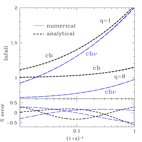
Figure 2: Analytic vs. numerical descriptions of neutrino infall for $f_{\nu}=0.3$, $f_{b}=0.01$, $\Omega_{0}=1$, $h=0.5$. Upper panel: Growth functions compared to the fully free-streaming time-dependence of $y^{1-p_{cb}}$; numerical CDM $+$ baryon fluctuations compared with growth function $D_{cb}$ (short-dashed lines) numerical CDM $+$ baryon $+$ neutrino density-weighted fluctuations compared with $D_{cb\nu}$ (long-dashed lines). No infall is represented by a horizontal line of amplitude 1 ($cb$) and $f_{cb}=0.69$ ($cb\nu$) here. Lower panel: relative error.

Furthermore, the density-weighted fluctuation

$$\delta_{cb\nu}=f_{cb}\delta_{cb}+f_{\nu}\delta_{\nu}$$ (14)

follows from the infall solution by noting that it converges above the free-streaming scale to $\delta_{cb}$ and below to $f_{cb}\delta_{cb}$. Thus

$$\delta_{cb\nu}(y,q;f_{\nu},f_{b},y_{d})=D_{cb\nu}(y,q;f_{\nu})\delta_{d}(q;f_{\nu},f_{b},y_{d})\,,$$ (15)

where

$$D_{cb\nu}(y,q;f_{\nu})=\left[f_{cb}^{0.7/p_{cb}}+\left({y\over 1+y_{\rm fs}(q;f_{\nu})}\right)^{0.7}\right]^{p_{cb}/0.7}y^{1-p_{cb}}.$$ (16)

In Fig. 2, we show that this form produces a good fit to the numerical results (lower set, long-dashed lines).

Finally, the horizon at the epoch when the neutrinos become nonrelativistic sets the maximal free-streaming scale. Beyond this scale, the neutrinos are always in the infall regime and the evolution of density fluctuations becomes independent of the neutrino fraction

$$\lim_{q\rightarrow 0}\delta_{cb}(y,q)={1\over 137q^{2}}y\Phi(0,q)\,.$$ (17)

The appearance of $y/(1+y_{\rm fs})$ in equation (12) assures the proper time dependence for the evolution in the large-scale limit. The growth functions are thus not subject to a small-scale approximation and remain valid for all $q$.

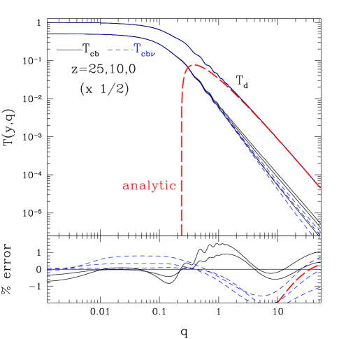
Figure 3: Demonstration of the existence of a time-independent master function. The transfer functions for the CDM $+$ baryon ($T_{cb}$) and CDM $+$ baryon $+$ neutrino ($T_{cb\nu}$) fluctuations at 3 different redshifts are divided by the growth factors $D_{cb}$ and $D_{cb\nu}$ respectively to obtain estimates of $T_{\rm master}$. That the 6 curves superimposed in the upper panel agree at the $1-2\%$ level (relative to $T_{cb}/D_{cb}$ at $z=0$, as shown in the lower panel) establishes the existence of the master function and verifies the accuracy of the growth functions. The analytic prediction for $T_{\rm master}$ (long-dashed line) converges to within $1\%$ of the numerical results at $q\gg 1$. The model here is $\Omega_{0}=1$, $h=0.5$, $f_{\nu}=0.4$, $f_{b}=0.2$.

5 Transfer Functions

We are now in a position to evaluate the transfer function, defined as

$$T_{i}(y,q)={\delta_{i}(y,q)\over\delta_{i}(y,0)}{\Phi(0,0)\over\Phi(0,q)}\,,$$ (18)

for the $i$th component of the matter. For the CDM $+$ baryon ($i=cb$) and the CDM $+$ baryon $+$ neutrino ($i=cb\nu$) systems, we obtain

$$T_{cb}(y,q;f_{\nu},f_{b},y_{d}) = y^{-1}D_{cb}(y,q;f_{\nu})T_{\rm master}(q;f_{\nu},f_{b},y_{d})\,,$$

$$T_{cb\nu}(y,q;f_{\nu},f_{b},y_{d}) = y^{-1}D_{cb\nu}(y,q;f_{\nu})T_{\rm master}(q;f_{\nu},f_{b},y_{d})\,,$$ (19)

where $T_{\rm master}$ has the small-scale limit of

$$\lim_{q\rightarrow\infty}T_{\rm master}(q;f_{\nu},f_{b},y_{d})={M_{d}(q)\over 14.4q^{2}}\,,$$ (20)

which follows from equations (7) and (17). It is important to note that relation (19) holds independently of the small-scale approximation: namely that once the growth factors $y^{-1}D_{i}$ are removed, the transfer functions depend only on a single time-independent function of $q$ related to perturbations in the CDM component at the drag epoch. This simplification holds only for $y\gg y_{d}$; near the drag epoch, the contribution of the decaying mode cannot be neglected. In Eisenstein & Hu (1997b), we exploit the existence of this master function to obtain the full time- and $q$-dependent transfer functions based on fitting formulae for $T_{\rm master}$.

We show a comparison between analytic and numerical results in Fig. 3. The numerical $T_{cb},T_{cb\nu}$ (lower curves, solid and dashed lines respectively) at 3 different redshifts are plotted here. The upper curve represents the master function $T_{\rm master}$ obtained through inverting the growth factor. Note that 6 different estimates of $T_{\rm master}$ obtained from $T_{cb}$ and $T_{cb\nu}$ are superimposed and agree at the $\sim 1-2\%$ level. Also shown is the small-scale prediction of equation (20) which converges rapidly for $q\gtrsim 1$.

Finally, note that the neutrino transfer function is implicitly defined as

$$T_{\nu}=f_{\nu}^{-1}(T_{cb\nu}-f_{cb}T_{cb})\,,$$ (21)

and its construction from the growth functions and $T_{\rm master}$ yields density-weighted errors on the same order as the other transfer functions, i.e. $(1-2\%)\times\,\delta_{cb\nu}/f_{\nu}\delta_{\nu}$.

6 Low Density Models

The formulae presented thus far are valid for $\Omega_{0}=1$ cosmologies. We have however shown that the transfer functions today can be expressed as the products of a growth function and a master function related to fluctuations at the drag epoch. At this earlier time, the cosmological constant and curvature have negligible effects on the dynamics. This implies that a simple modification of the growth function at late times to account for $\Omega_{0}\neq 1$ effects will suffice for a complete description.

Let us recall that on the largest scales, where neutrino free streaming and radiation pressure gradients are negligible, fluctuations grow as (Heath  1977)

$$D(y;\Omega_{0},\Omega_{\Lambda})={5\over 2}g(y)\int^{y}{dx\over x^{3}g(x)^{3}}\,,$$ (22)

where

$$g^{2}(y)=y^{-3}+y^{-2}y_{0}^{-1}(1-\Omega_{0}-\Omega_{\Lambda})/\Omega_{0}+y_{0}^{-3}\Omega_{\Lambda}/\Omega_{0}\,,$$ (23)

with $y_{0}=(1+z_{\rm eq})$. Analytic forms for the $\Omega_{\Lambda}=0$ and $\Omega_{0}+\Omega_{\Lambda}=1$ cases are given in Groth & Peebles (1975) and Bildhauer et al. (1992) respectively. The normalization of the growth rate has been chosen so that $D=y$ at early times. Moreover, equation (22) states that after matter ceases to dominate the expansion rate, fluctuation growth halts.

By matching these asymptotic limits, we can approximate the growth function in the presence of neutrinos by the replacement of $y$ with $D$, i.e.

$$D_{cb}(y,q;f_{\nu},\Omega_{0},\Omega_{\Lambda}) = \left[1+\left(D(y)\over 1+y_{\rm fs}(q)\right)^{0.7}\right]^{p_{cb}/0.7}D^{1-p_{cb}}(y)\,,$$ (24)

$$D_{cb\nu}(y,q;f_{\nu},\Omega_{0},\Omega_{\Lambda}) = \left[f_{cb}^{0.7/p_{cb}}+\left(D(y)\over 1+y_{\rm fs}(q)\right)^{0.7}\right]^{p_{cb}/0.7}D^{1-p_{cb}}(y)\,,$$ (25)

where of course $D(y)=D(y;\Omega_{0},\Omega_{\Lambda})$ implicitly. Likewise, the transfer functions become

$$T_{cb}(y,q) = D^{-1}(y)D_{cb}(y,q)T_{\rm master}(q)\,,$$

$$T_{cb\nu}(y,q) = D^{-1}(y)D_{cb\nu}(y,q)T_{\rm master}(q)\,.$$ (26)

We show an example in Fig. 4. The model has been chosen to have $\Omega_{0}=0.25$, $\Omega_{\Lambda}=0.75$ with the same $\Omega_{0}h^{2}$, $f_{b}$ and $f_{\nu}$ as Fig. 3 and hence the same $T_{\rm master}$. The invariance of the master function is demonstrated by overplotting estimates from $T_{cb}$ and $T_{cb\nu}$ in this model and from $T_{cb}$ of Fig. 3. The lower panel shows the fractional difference of the former with respect to the latter.

In principle, the fact that infall freezes out at a later redshift in a $\Lambda$ vs. open cosmology of the same $\Omega_{0}$ allows one to distinguish between these two alternatives by the shape of the transfer function at a single redshift alone. Massive neutrinos therefore break the shape degeneracy of the transfer function in low-density universes. However, since this effect is only significant if $\Omega_{0}\ll 1$, the more important fact is that growth in the matter-dominated epoch depends on $(1-\Omega_{\nu}/\Omega_{0})$ and hence even a relatively small density in neutrinos can make a dramatic effect on the growth rates in a low-density universe. Fig. 4 demonstrates that $\Omega_{\nu}=0.1$ in an $\Omega_{0}=0.25$ universe gives the same magnitude effects as $\Omega_{\nu}=0.4$ in an $\Omega_{0}=1$ universe. Upper limits on $\Omega_{\nu}$ from small-scale fluctuations thus tighten for low density universes (Primack et al.  1995).

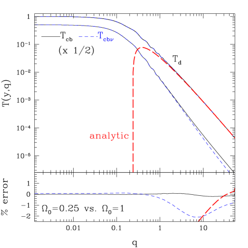
Figure 4: Demonstration of the invariance of the master function ($T_{\rm master}$) under changes in the cosmological constant $\Lambda$. The model has the same $\Omega_{0}h^{2}$, $f_{b}$ and $f_{\nu}$ as Fig. 3 at $z=0$ but with $\Omega_{0}=0.25$. Division of $T_{cb}$ and $T_{cb\nu}$ by the growth functions returns the master function $T_{\rm master}$ over which the estimate of Fig. 3 and the small-scale analytic solution are plotted (top panel). The errors are plotted relative to $T_{\rm master}$ from the $T_{cb}$, $z=0$ estimate of Fig. 3 and show agreement at the $1-2\%$ level (bottom panel).

7 Discussion

We have presented small-scale solutions to the linear evolution of perturbations in a cold $+$ hot $+$ baryonic dark matter cosmology. They converge to within $1\%$ of the numerical solutions for $q\gg 1$ and $q\gg q_{\rm fs}$ and are expressed in terms of hypergeometric functions in the Appendix. We have also given simplified forms in the main text, employing only algebraic functions, which are valid for $\Omega_{b}+\Omega_{\nu}\lesssim 0.6\Omega_{0}$ and $\Omega_{0}h^{2}\gtrsim 0.1$. Baryons play a significant role in MDM cosmologies since dark-matter perturbations are density weighted and depend on $\Omega_{b}/(\Omega_{0}-\Omega_{\nu})$ not $\Omega_{b}/\Omega_{0}$. Likewise neutrinos in a low-density universe yield enhanced effects since growth rates depend on $\Omega_{\nu}/\Omega_{0}$.

By comparing analytic and numerical results at $q\lesssim q_{\rm fs}$, we have isolated the effects of neutrino infall and described them to an accuracy of $1-2\%$ by time- and wavenumber-dependent growth factors for the CDM and total matter. The freeze-out of infall at late times when $\Lambda$ or curvature come to dominate can similarly be taken into account. We have shown that these growth factors are valid beyond the small-scale approximation.

The full time and wavenumber dependent transfer functions for the CDM and total matter can thus be described as a product of these growth factors and a single function of wavenumber related to the amplitude of fluctuations at the Compton drag epoch that in turn depends on $\Omega_{0}h^{2}$, $\Omega_{\nu}/\Omega_{0}$, $\Omega_{b}/\Omega_{0}$, and the number of degenerate neutrino species. We leave a quantitative description of this master function and implications for constraints on $\Omega_{\nu}$ to a companion piece (Eisenstein & Hu  1997b).

Acknowledgments: W.H. and D.J.E. are supported by NSF PHY-9513835. W.H. was additionally supported by the W.M. Keck Foundation. Numerical results were extracted from the CMBfast package of Seljak & Zaldarriaga (1996) v. 2.3.

Appendix A Derivation of the Small Scale Solution

Following the analytic approach of HS (96), one can solve the equation of motion for the CDM on small scales where the gravitational effects of the MDM can be neglected. The idea is to separate the evolution before and after the drag epoch. Before the drag epoch, the gravitational effects of the baryons can be ignored below the sound horizon as they are pressure supported by the photons. The equation of motion then becomes

$$\ddot{\delta}_{c}+{\dot{a}\over a}\dot{\delta}_{c}={3\over 2a}f_{c}\Omega_{0}H_{0}^{2}\delta_{c}\,,$$ (A1)

where overdots indicate derivatives with respect to conformal time $\eta$. Unfortunately, the complicated equation of state of massive neutrinos prevents the time evolution of the scale factor $a(\eta)$ from being written down in closed form. However, we know that the neutrinos behave as radiation at early times when $T_{\nu}\gg m_{\nu}$ and as matter at late times when $T_{\nu}\ll m_{\nu}$. These limits are identical to those found if one considered the neutrinos to be massless and added their mass to that of the non-relativistic matter. It is therefore a reasonable first approximation to leave the background evolution unmodified by the replacement of a portion of the non-relativistic matter with massive neutrinos, i.e.

$$\eta=2(\Omega_{0}H_{0}^{2})^{-1/2}(1+z_{\rm eq})^{-1/2}\left(\sqrt{1+y}-1\right)\,,$$ (A2)

where $y=(1+z_{\rm eq})/(1+z)$. Here, $z_{\rm eq}$ [eq. (1)] assumes three massless neutrino species with the usual thermal history. We neglect cosmological constant and curvature effects here (see §6). This form otherwise errs only between $z_{\rm eq}$ and the epoch at which the neutrinos become non-relativistic. Our approach will be to use this approximation to solve the small-scale limit analytically and then correct for a $\lesssim 5\%$ modification due to changes in the expansion rate.

With this approximation, equation (A1) can be rewritten in terms of $y\equiv(1+z_{\rm eq})/(1+z)$ as

$${d^{2}\over dy^{2}}\delta_{c}+{(2+3y)\over 2y(1+y)}{d\over dy}\delta_{c}={3\over 2y(1+y)}f_{c}\delta_{c}\,.$$ (A3)

As shown in HS (96), the general solution to this equation is given through Gauss’s hypergeometric function $F$ (also written ${}_{2}F_{1}$)

$$U_{i}=(1+y)^{-\alpha_{i}}F(\alpha_{i},\alpha_{i}+{1\over 2},2\alpha_{i}+{1\over 2};{1\over 1+y})\,,$$ (A4)

where $i=1,2$ and

$$\alpha_{i}={1\mp\sqrt{1+24f_{c}}\over 4}\,,$$ (A5)

with $-$ and $+$ for $i=1$ and $2$, respectively. It is useful to note that $\lim_{y\rightarrow\infty}U_{i}=y^{-\alpha_{i}}$ and thus the two solutions represent the growing and decaying mode for $i=1,2$ respectively. Clearly, $\alpha_{1}+\alpha_{2}=1/2$.

We obtain the amplitude of the growing and decaying mode by matching onto the $y\ll 1$ solution of HS (96) eq. (B12)

$$\delta_{c}=9.50\ln(9.24qy)\Phi(0,q)\,,\qquad y\ll 1\,,$$ (A6)

to find

$$\delta_{c}(y,q)=9.50[A_{1}(q)U_{1}(y)+A_{2}(q)U_{2}(y)]\Phi(0,q)\qquad y<y_{d}\,,$$ (A7)

where the matching coefficients are

$$A_{1}(q)={\Gamma(\alpha_{1})\Gamma(\alpha_{1}+1/2)\over\Gamma(2\alpha_{1}+1/2)2\pi\cot(2\pi\alpha_{1})}\left[\ln(9.04q)+2\psi(1)-2\psi(1-2\alpha_{1})-2\ln 2\right]\,,$$ (A8)

with $\psi(x)=\Gamma^{\prime}(x)/\Gamma(x)$. The expression for $A_{2}$ follows from equation (A8) with the replacement $1\rightarrow 2$ in the subscripts.

Equation (A7) takes the evolution up to the drag epoch. After the drag epoch, the baryons are released from the photons and behave as cold dark matter. The equation of motion for the combined CDM+baryon system is the same as equation (A3) but with the replacements

$$\delta_{c} \rightarrow {f_{c}\over f_{cb}}\delta_{c}+{f_{b}\over f_{cb}}\delta_{b}\equiv\delta_{cb}\,,$$

$$f_{c} \rightarrow f_{cb}\,,$$ (A9)

and therefore has the same solutions as given by equation (A4) with arguments

$$\widetilde{\alpha}_{i}={1\pm\sqrt{1+24f_{cb}}\over 4}\,.$$ (A10)

The full solution for $\delta_{cb}$ is now found by matching the solution of equation (A7) onto the new growing and decaying modes. Since the decaying mode becomes unimportant for $y\gg y_{d}$,

$$\delta_{cb}(y,q)=9.50M_{d}(q)\widetilde{U}_{1}(y)\Phi(0,q)\,,$$ (A11)

where

$$M_{d}(q)={f_{c}\over f_{cb}}\left({\widetilde{U}_{2}^{\prime}[A_{1}U_{1}+A_{2}U_{2}]-\widetilde{U}_{2}[A_{1}U_{1}^{\prime}+A_{2}U_{2}^{\prime}]\over\widetilde{U}_{1}\widetilde{U}_{2}^{\prime}-\widetilde{U}_{1}^{\prime}\widetilde{U}_{2}}\right)\Bigg{|}_{y=y_{d}}\,,$$ (A12)

gives the matching condition.

Furthermore, the baryons fall into CDM potential wells at the drag epoch and subsequently follow them so that

$$\delta_{cb}=\delta_{c}=\delta_{b}\,,\qquad y\gg y_{d}\,.$$ (A13)

For high $\Omega_{0}h^{2}\gtrsim 0.1$ (or $h\gtrsim 0.3$), $y_{d}\gg 1$ so that the decaying-mode contribution to equation (A11) coming through $U_{2}$ is negligible. Furthermore the growing mode can be expanded in powers of $(1+y_{d})^{-1}$ as

$$M_{d}(q) \approx {f_{c}\over f_{cb}}{2(\widetilde{\alpha}_{1}+\alpha_{1})-1\over 4\widetilde{\alpha}_{1}-1}(1+y_{d})^{\widetilde{\alpha}_{1}-\alpha_{1}}$$ (A14)

$$\times\left[1+(1+y_{d})^{-1}{\alpha_{1}-\widetilde{\alpha}_{1}\over 2}\left(1+{1\over{(4\alpha_{1}+1)(4\widetilde{\alpha}_{1}-3)}}\right)\right]A_{1}(q)\,.$$

The approximation holds for $f_{c}\gtrsim 0.2$. Note that the apparent divergence at $f_{c}=0.125$ or $\alpha_{1}=-1/4$ disappears once the decaying mode is properly included.

The quantity $A_{1}$ can either be evaluated from equation (A8) or approximated as

$$A_{1}(q)=\left[{1-0.553f_{\nu b}+0.126f_{\nu b}^{3}}\right]\ln(1.84\beta_{c}q)\,,$$ (A15)

with

$$\beta_{c}\equiv\exp[-2\psi(2\alpha_{2})-2\psi(3)]\approx[1-0.949f_{\nu b}]^{-1}\,,$$ (A16)

which is valid at the $1\%$ level for $f_{\nu b}\lesssim 2/3$. Finally, we correct for the change in the background expansion rate by comparing equation (A11) to an numerical integration of equation (A1) and find the small correction

$$A_{1}(q)\rightarrow{A_{1}(q)\over 1-0.193\sqrt{f_{\nu}N_{\nu}}+0.169f_{\nu}N_{\nu}^{0.2}}\,,$$ (A17)

for $f_{\nu}\lesssim 0.6$. With the identities $\alpha_{1}=p_{c}-1$ and $\widetilde{\alpha}_{1}=p_{cb}-1$, the derivation of the small-scale evolution [eq. (4)] is now complete.

References

- (1) Bildhauer, S., Buchert, T., & Kasai, M. 1992, A&A, 263, 23
- (2) Bond, J.R., Efstathiou, G., & Silk, J. 1980, Phys. Rev. Lett., 45, 1980
- (3) Bond, J.R., & Szalay, A.S. 1983, ApJ, 274, 443
- (4) David, L.P., Jones, C., & Forman, W. 1995, ApJ, 445, 578
- (5) Dodelson, S., Gates, E., Stebbins, A. 1996, ApJ, 467, 10 [astro-ph/9509147]
- (6) Eisenstein, D.J., & Hu, W. 1997a, ApJ (submitted) [astro-ph/9709112]
- (7) Eisenstein, D.J., & Hu, W. 1997b, ApJ (submitted)
- (8) Fixsen, D. et al. 1996, ApJ, 473, 576 [astro-ph/9605054]
- (9) Groth, E.J., & Peebles, P.J.E. 1975, A&A, 41, 143
- (10) Heath, D.J. 1977, MNRAS, 179, 351
- (11) Hu, W., Scott, D., Sugiyama, N., & White, M. 1995, Phys. Rev. D., 52, 5498 [astro-ph/9505043]
- HS (96) Hu, W., & Sugiyama, N. 1996, ApJ, 471, 542 (HS96) [astro-ph/9510117]
- (13) Kauffmann, G., & Charlot, S. 1994, ApJ, 430, L97 [astro-ph/9402015]
- (14) Klypin, A. Borgani, S., Holtzman, J.A., Primack, J.R. 1995, ApJ, 441, 1 [astro-ph/9407011]
- (15) Ma, C.-P. 1996, ApJ, 471, 13 [astro-ph/9605198]
- (16) Ma, C.-P., & Bertschinger, E. 1995, ApJ, 455, 7 [astro-ph/9506072]
- (17) Ma, C.-P., Bertschinger, E., Hernquist, L., Weinberg, D.H., & Katz, N. 1997, ApJ, 484 L1 [astro-ph/9705113]
- (18) Mo, H.J., & Fukugita, M. 1996, ApJL, L9 [astro-ph/9604034]
- (19) Mo, H.J., & Miralda-Escudé, J. 1994, ApJ, 430, L25 [astro-ph/9402014]
- (20) Primack, J.R., Holtzman, J., Klypin, A., Caldwell, D.0. 1995, Phys. Rev. Lett., 74, 2160 [astro-ph/9411020]
- (21) Rugers, M., & Hogan, C.J. 1996, ApJ, 459, L1 [astro-ph/9512004]
- (22) Seljak, U., & Zaldarriaga, M. 1996, ApJ, 469, 437 [astro-ph/9603033]
- (23) Steidel, C.C., Giavalisco, M., Pettini, M. Dickinson, M., & Adelberger, K.L. 1996, ApJL, 462, L17 [astro-ph/9602024]
- (24) Sugiyama, N. 1995, ApJS, 100, 281 [astro-ph/9412025]
- (25) Tytler, D., Fan, X.M., & Burles, S. 1996, Nature, 381, 207 [astro-ph/9603069]
- (26) Walker, T.P., Steigman, G., Kang, H., Schramm, D.M., Olive, K.A. 1991, ApJ, 376, 51
- (27) Weinberg, D.H., Miralda-Escudé, J., Hernquist, L., & Katz, N. 1997, submitted to ApJ [astro-ph/9701012]
- (28) White, S.D.M., Navarro, J.F., Evrard, A.E., & Frenk, C.S. 1993, Nature, 366, 429