Photo-evaporation of clumps in Planetary Nebulae

Abstract

We study the evolution of dense neutral clumps located in the outer parts of planetary nebulae. These clumps will be photo-ionized by the ionizing radiation from the central star and change their structure in the process. The main effect of the ionization process is the setting up of a photo-evaporation flow and a shock running through the clump. Once this shock has moved through the entire clump it starts to accelerate because of the ‘rocket effect’. This continues until the entire clump has been photo-ionized. We present an analytic model for the shock and accelerating phases and also the results of numerical simulations which include detailed microphysics. We find a good match between the analytic description and the numerical results and use the numerical results to produce some of the clump’s observational characteristics at different phases of its evolution. We compare the results with the properties of the fast moving low ionization knots (ansae or FLIERs) seen in a number of planetary nebulae. We find that the models match many of the kinematic and emission properties of FLIERs.

1 Introduction

A fraction of Planetary Nebulae (PNe) show small scale structures which differ considerably from their surroundings in either line ratios or radial velocity or both. When these appear in pairs in along the symmetry axis of the nebulae they are often referred to as ‘ansae’, or when there is a clear velocity difference, by the acronym of FLIERs (Fast Low Ionization Emission Regions), first introduced by Balick et al. (1993). The defining observational properties of FLIERs are that they should be bright in low ionization lines, located along the major axis of the PNe, and have a higher velocity than their environment. There are many cases which fulfill the first two criteria but for which no kinematic data is available, leaving their status as FLIERs uncertain. Examples of these can be found in Corradi et al. (1996), who took ratios of H$\alpha$+[N II] to [O III] to bring out many low ionization regions in PNe. Often the ansae are only marginally resolved in ground based images; in some cases they are clearly elongated into ‘tails’. In some other cases one observes a whole series of ansae, as for example in Fg 1 (López et al. (1993), Palmer et al. (1996)). See Mellema (1996) and López (1997) for reviews on what appear to be collimated outflows from PNe.

Among the best studied FLIERs are the ones in NGC 3242, NGC 6543, NGC 6826, NGC 7009, and NGC 7662, and these are the ones that have also been selected for imaging with the HST (Harrington (1995); Balick et al. (1997)). Ground based studies of the kinematics of the FLIERs in these PNe can be found in Balick et al. (1987) and Miranda & Solf (1992). The radial velocities of these FLIERs are typically around 30 to 50 km s^-1. Balick et al. (1993) and Balick et al.  (1994) studied their spectroscopic properties in some detail. They found that the derived densities and temperatures are not very different from those of the environment, a surprising result given their conspicuous appearance in the low ionization lines. The higher ionization species are found at the side facing the star, indicating that photo-ionization determines the ionization stratification. Because of the observed velocities one would expect a bow shock (and higher ionization species associated with it) at the end facing away from the star, but this is not observed.

The HST results (a preview of which can be found in Weinberger & Kerber (1997)) show a considerable amount of detail and the analysis has not yet been completed. The images seem to show little arcs either pointing towards or away from the star, and more diffuse regions also pointing both towards and away from the star.

The actual configuration of the FLIERs is not at all clear. The groundbased observations suggested fast moving clumps being photo-ionized from behind, but the morphologies seen in the HST images do not seem to support this. The tails pointing away from the stars (very clearly seen in NGC 3242), suggest rather the reverse: a clump being hit by a wind from behind. However there is no other evidence for such a wind. At this point it seems hard to propose a definite model for the FLIERs.

One of the surprising properties of the FLIERs is their brightness in [N II]. The [N II]$\lambda 6583$ line is normally as strong as or stronger than the nearby H$\alpha$ line. This is usually interpreted as being due to a high nitrogen abundance, which implies that the FLIERs were formed from stellar material enriched through the CNO-cycle.

To study the structure of FLIERs we developed a hydrodynamics code which includes the most relevant micro-physical processes, such as radiative cooling and photo-ionization. But as was stated above it is not clear what to choose for initial conditions. There appear to be two cases which could be used as a FLIER model. Both involve a dense clump moving away from the central star, but in the one case the clump is moving faster than its environment, and in the other slower. The first case is the ‘classical’ FLIER model, but the new HST results support the second model.

What both cases have in common is the gradual photo-ionization of the clump. We therefore decided to study this effect first, for the moment neglecting the effect of any velocity difference with the environment. In fact, the photo-ionization will cause an acceleration of the clump due to the so called rocket effect (Oort & Spitzer  1995). If the rocket effect is very efficient, it might not even be necessary to invoke a wind; the clump would reach FLIER-like velocities within its life time ($\sim 1000$ years, see Balick et al. 1987).

We therefore study here the evolution of a dense clump being photo-ionized by the stellar radiation. In Sect. 2 we present an analytic model for the shape and evolution of such a clump. In Sect. 3 we describe the numerical method that we used to compute the models shown in Sect. 4. In Sect. 5 we compare the numerical results to the analytic ones, and in Sect. 6 we compare them to the observations. In Sect. 7 we summarize the conclusions of the paper.

2 Analytic model

2.1 General description

The evolution of a dense clump being photo-ionized consists of two phases, the collapse or implosion phase and the cometary phase. These processes have been studied by many authors, starting with Oort & Spitzer  (1955). The three most recent papers are those of Bertoldi (1989) on the collapse phase, Bertoldi & McKee (1990) on the cometary phase and Lefloch & Lazareff (1994) on both. The introduction in Bertoldi (1989) contains a good review of all the previous work.

In the collapse phase an ionization front of type D forms, preceded by a shock wave which travels through the clump, gradually compressing, accelerating and heating it. At the ionization front, material is ionized and thrown out in a photo-evaporation flow. Once the shock has moved through the entire clump, it enters the cometary phase in which the whole clump starts to accelerate due to the rocket effect caused by the photo-evaporation flow.

2.2 The collapse phase

Let us consider the initial acceleration of a spherical clump by the interaction with the impinging ionizing radiation field. The clump has an initial mass $M_{\rm i}$, density $\rho_{\rm i}$, radius $R_{\rm i}$ and sound speed $c_{\rm i}$. Let $M_{\rm s}$ be the mass of the shocked material and $v$ its velocity (see Fig. 1). The equation of motion of this mass is

$$M_{\rm s}{dv\over dt}=P_{0}A_{\rm I}-\rho_{\rm i}v_{\rm s}A_{\rm S}v\,,$$ (1)

and the equation of mass conservation is

$${dM_{\rm s}\over dt}=-m\,F\,A_{\rm I}+\rho_{\rm i}v_{\rm s}A_{\rm S}\,,$$ (2)

where $v_{\rm s}$ is the shock velocity, and $A_{\rm I}$ and $A_{\rm S}$ are the effective areas of the ionization front and the shock front (respectively), shown schematically in Fig. 1. $P_{0}$ is the pressure driving the shock, which results from a D-critical ionization front. $P_{0}=2\,F\,m\,c_{1}$ (see Sect. 2.3), in which $F$ is the ionizing photon flux reaching the ionization front and $c_{1}$ is the isothermal sound speed of the ionized material. We assume $P_{0}$ to be constant. The average mass per atom or ion is taken to be $m\approx 1.3\,m_{\rm H}$ (where $m_{\rm H}$ is the mass of hydrogen). If $A_{\rm I}\approx A_{\rm S}$, Eq. 1 has the trivial solution $v=v_{0}={\rm constant}$, with quantities given by

$$P_{0}=\rho_{\rm i}v_{\rm s}v_{0}\,,$$ (3)

$$\rho_{\rm i}v_{\rm s}=\rho_{0}\,(v_{\rm s}-v_{0})\,,$$ (4)

$$\rho_{\rm i}\left({c_{\rm i}}^{2}+{v_{\rm s}}^{2}\right)=\rho_{0}\,\left[{c_{0}}^{2}+(v_{\rm s}-v_{0})^{2}\right]\,,$$ (5)

where $\rho_{0}$ is the density of the shocked material, and $c_{0}$ its sound speed. This sound speed is fixed by the radiative losses in the post-shock region. If we now assume that $c_{\rm i}\ll v_{\rm s}$, Eqs. 4 and 5 give

$$v_{\rm s}\approx v_{0}+{{c_{0}}^{2}\over v_{0}}\,,$$ (6)

$$\rho=\rho_{\rm i}\,\left(1+{{v_{0}}^{2}\over{c_{0}}^{2}}\right)\,.$$ (7)

Substituting Eq. 6 into 3 one finally obtains the (constant) velocity $v_{0}$ of the shocked material, which is given by

$$v_{0}=\left({P_{0}\over\rho_{\rm i}}-{c_{0}}^{2}\right)^{1/2}\,,$$ (8)

so that the position of the clump as a function of time is $x_{\rm IF}=v_{0}\,t$. The shock goes through the diameter of the clump in a time

$$t_{0}={{2\,R_{\rm i}}\over v_{\rm s}}\,,$$ (9)

after which the cometary phase starts (described in the next subsection). We now show that by time $t_{0}$ a substantial amount of the clump material has already been photoionized.

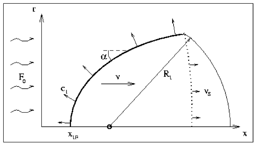
Figure 1: Schematic diagram showing the interaction of a dense clump of initial radius $R_{\rm i}$ with an impinging ionizing photon flux $F_{0}$. The back-reaction of the photo-evaporation flow (driven out at a sonic velocity $c_{1}$) drives a shock (of velocity $v_{\rm s}$) into the clump. The shocked clump material moves away from the photon source at a velocity $v$. The position of the ionization front along the symmetry axis is $x_{\rm IF}$. The ionization front is indicated with a thick line, the shock front with a dotted line

Using the $A_{\rm I}\approx A_{\rm S}$ approximation in Eq. 2, one can conclude that the ratio between the neutral clump mass at the end of this phase, $M_{0}$, and its initial mass is

$${M_{0}\over M_{\rm i}}\approx 1-{{m\,F}\over\rho_{\rm i}v_{\rm s}}\,.$$ (10)

The mass $M$ of the clump can be obtained from the differential equation

$${dM\over dt}=-m\,F\,A_{\rm I}\,.$$ (11)

In order to integrate this equation, let us consider the length $l$ associated with the area $A_{\rm I}$ : $l\propto{A_{\rm I}}^{1/2}$. Then, for a uniform density clump we have $M\propto l^{3}$, and therefore we can write

$$A_{\rm I}=\beta\,M^{2/3}\,,$$ (12)

where we assume that $\beta$ is constant with time. However, this assumption of a constant $\beta$ is only strictly true for a clump of time-independent average density, which is not the case as the clump has both undisturbed and shocked components (see Fig. 1) of different densities, and the proportion of mass in these two components evolves with time. However, as we will see when comparing the analytic model with the numerical results in Sect. 5, this approximation appears to give a reasonable description of the evolution of the clump in the collapse phase.

Using Eq. 12 we can integrate 11 to obtain

$$M(t)=M_{\rm i}\,\left(1-\beta{m\,F\over 3\,{M_{\rm i}}^{1/3}}t\right)^{3}\,,$$ (13)

where we have taken $M=M_{\rm i}$ for $t=0$ as the initial condition.

To find the constant $\beta$, we use the condition $M=M_{0}$ (given by Eq. 10) for $t=t_{0}$. The result is

$$\beta={3\,{M_{\rm i}}^{1/3}\over m\,F\,t_{0}}\left[1-\left({M_{0}\over M_{\rm i}}\right)^{1/3}\right]\,.$$ (14)

Substituting Eq. 14 into 13, we finally obtain the mass of the clump as a function of time

$$M(t)=M_{\rm i}\,\left\{1-\left[1-\left({M_{0}\over M_{\rm i}}\right)^{1/3}\right]{t\over t_{0}}\right\}^{3}\,,$$ (15)

where the term $M_{0}/M_{\rm i}$ can of course be substituted by the right hand side of Eq. 10. The flux $F$ during the collapse phase is approximately given by Eq. 34 (see below) with $R_{\rm IF}=R_{\rm i}$.

2.3 The cometary phase

In this section, we present a description of the ‘cometary phase’, which begins when the shock has moved through the entire clump. At this time, $t_{0}$ (Eq. 9), the shocked clump has a mass $M_{0}$ (Eq. 10), and is moving at a velocity $v_{0}$ (Eq. 8).

Let us assume that the shocked clump has a uniform temperature $T_{0}$ (and therefore a uniform isothermal sound speed $c_{0}$) and that it is subject to a uniform acceleration $a$. The pressure and density stratifications then follow from the condition of hydrostatic equilibrium

$${dP_{0}\over dx}=-a\,\rho_{0}\,,$$ (16)

which gives pressure and density stratifications of the form

$$P_{0}(x)=\rho_{0}(x)\,{c_{0}}^{2}=P_{0}(0)\,{\rm e}^{-x/h}\,,$$ (17)

where $P_{0}(0)$ is the pressure at the tip of the clump (at $x=0$), and $h$ is the scale height, which is given by

$$h={{c_{0}}^{2}\over a}\,.$$ (18)

The $x$-axis points away from the head of the clump in a direction parallel to the ionizing photon flux (see the schematic diagram of Fig. 1).

Let us now assume that the clump is embedded in an impinging ionizing radiation field, so that it is enveloped by an ionization front which moves into the clump. Let $u_{0}$ and $u_{1}$ be the velocities of the neutral and ionized flows with respect to the ionization front. The mass and momentum conservation equations then give us

$$\rho_{1}u_{1}=\rho_{0}\,u_{0}\,,$$ (19)

$$P_{1}+\rho_{1}{u_{1}}^{2}=P_{0}+\rho_{0}\,{u_{0}}^{2}\,,$$ (20)

where $P_{1}$ and $\rho_{1}$ are the pressure and density in the ionized material, and $P_{0}$ and $\rho_{0}$ are the pressure and density on the neutral side of the front, which are given by Eq. 17. From Eqs. 19 and 20, we then obtain

$$P_{0}(x)=P_{1}+\rho_{1}{u_{1}}^{2}\left(1-{u_{0}\over u_{1}}\right)\,.$$ (21)

We define $c_{1}$ to be the isothermal sound speed in the ionized material, and assume that $u_{1}=c_{1}$, as would be the case for a D-critical ionization front. Then $P_{1}=\rho_{1}{u_{1}}^{2}$, and therefore

$${u_{0}\over u_{1}}=1-\sqrt{1-\left({c_{0}\over c_{1}}\right)^{2}}\approx{1\over 2}\left({c_{0}\over c_{1}}\right)^{2}\ll 1\,.$$ (22)

Eq. 21 can then be written as

$$P_{0}(x)\approx 2\rho u_{0}c_{1}\,,$$ (23)

where we have also used Eq. 19.

Let us now consider a point on the surface of the clump, as shown in the schematic diagram of Fig. 1. Considering that each ionizing photon impinging on the ionization front results in a photoionization of a further atom of the clump, it follows that

$$F\,m\,\sin\alpha\approx\rho\,u_{0}\,,$$ (24)

where $F$ is the (uniform) impinging photon flux, $m$ is the average mass per atom of the clump ($\approx 1.3\,m_{\rm H}$) and $\alpha$ is the angle defined in Fig. 1. In this we ignore the differences in the ionization structure of hydrogen and helium. Substituting Eq. 24 into 23, we obtain

$$P_{0}(x)=2\,F\,c_{1}\,m\,\sin\alpha\,,$$ (25)

and from Eq. 17

$$P_{0}(0)=2\,F\,c_{1}\,m\,,$$ (26)

leading to the following differential equation for $r$, the cylindrical radius of the clump at a position $x$,

$${dr\over dx}=\left({\rm e}^{2x/h}-1\right)^{-1/2}\,.$$ (27)

Integrating Eq. 27 with the boundary condition $r=0$ for $x=0$, one obtains

$$r=h\,\arctan\left[\sqrt{{\rm e}^{2x/h}-1}\right]\,,$$ (28)

which gives the shape of the clump. This solution for the shape of a photo-evaporating clump is very similar to the solution for a clump accelerating due to a passing wind (de Young & Axford (1967)), normally referred to as a plasmon. We will therefore also refer to the photo-evaporating clump in the cometary phase as a plasmon.

The net force ${\cal F}_{x}$ in the $x$-direction and the mass $M$ of the clump follow from the integrations

$${\cal F}_{x}=\int_{0}^{\pi h/2}2\pi r\,P_{0}(x)\,dr\,,$$ (29)

$$M=\int_{0}^{\infty}\pi r^{2}\rho_{0}(x)\,dx\,.$$ (30)

Using Eqs. 17 and 28, one can integrate Eqs. 29 and 30 to obtain

$${\cal F}_{x}=\left(1-{2\over\pi}\right)\,\pi^{2}P_{0}(0)h^{2}\,,$$ (31)

$$M=\left(1-{2\over\pi}\right)\,\pi^{2}{P_{0}(0)\over{c_{0}}^{2}}h^{3}\,,$$ (32)

which enable us to recover Eq. 18 by taking the ratio $a={{\cal F}_{x}/M}={{c_{0}}^{2}/h}$. Equation 32 gives the mass of the clump in terms of the scale height (or viceversa).

The ionizing photon flux $F$ reaching the ionization front is in general smaller than the flux $F_{0}$ delivered by the star at the position of the clump. The flow produced at the ionization front, streaming out of the clump towards the star absorbs some of the impinging photons. The difference between $F_{0}$ and $F$ can be expressed as (Spitzer (1978)),

$$F_{0}-F={\alpha_{\rm R}F^{2}R_{\rm IF}\over 3\,{c_{1}}^{2}}\,,$$ (33)

where $\alpha_{\rm R}$ is the recombination coefficient, and $R_{\rm IF}$ is the radius of the curved ionization front. Although Eq. 33 has an exact solution for $F$ in terms of $F_{0}$ and $R_{\rm IF}$, in order to proceed analytically with the equations of motion for the clump it is necessary to use the approximate solution

$$F\approx{F_{0}\over{\left(1+{\alpha_{\rm R}F_{0}R_{\rm IF}\over 3\,{c_{1}}^{2}}\right)^{1/2}}}\,,$$ (34)

which deviates from the exact solution of Eq. 33 by less than 15%. For the radius of the ionizing front in Eq. 34, we will use the radius of curvature of the tip of the clump, which is equal to the scale height $h$.

The initial mass $M_{0}$ and the corresponding scale height $h_{0}$ are related through Eq. 32, which gives

$$M_{0}=\left(1-{2\over\pi}\right){\pi^{2}\over{c_{0}}^{2}}\left(2\,F_{0}c_{1}m\right){{h_{0}}^{3}\over{\left(1+{\alpha_{\rm R}F_{0}h_{0}\over 3\,{c_{1}}^{2}}\right)^{1/2}}}\,,$$ (35)

where we have also used Eqs. 26 and 34.

The rate of change of the mass of the plasmon is related to the impinging ionizing photon flux through

$${dM\over dt}=-F\,m\,\pi\,\left({\pi\over 2}h\right)^{2}\,,$$ (36)

where $\pi h/2$ is the outer radius of the projection of the plasmon onto a plane perpendicular to the symmetry axis (cf. Eq. 11). Equating Eq. 36 to the time derivative of Eq. 32 and using Eq. 34, one finds a differential equation for the time evolution of the scale height $h$

$${d\tilde{h}\over d\tilde{t}}=-{{6(1+\eta\tilde{h})}\over{6+5\eta\tilde{h}}}\,,$$ (37)

in terms of the dimensionless variables $\tilde{h}\equiv h/h_{0}$ and $\tilde{t}=t/t_{*}$, where

$$t_{*} \equiv {v_{*}h_{0}\over{c_{0}}^{2}}\,,$$ (38)

$$v_{*} \equiv {24\over\pi}\left(1-{2\over\pi}\right)\,c_{1}\,,$$ (39)

$$\eta \equiv {\alpha_{\rm R}F_{0}h_{0}\over 3\,{c_{1}}^{2}}\,.$$ (40)

Equation 37 can be integrated with initial conditions $\tilde{h}=1$ for $\tilde{t}=\tilde{t}_{0}\,(\equiv t_{0}/t_{*})$ to obtain

$${5\over 6}\left(1-\tilde{h}\right)+{1\over 6\eta}\,\ln\left({{1+\eta}\over{1+\eta\tilde{h}}}\right)=\tilde{t}-\tilde{t_{0}}\,.$$ (41)

It follows from Eq. 41 that the clump becomes fully ionized (that is, $\tilde{h}=0$) at a time

$$\tilde{t}_{\rm m}=\tilde{t}_{0}+{5\over 6}+{1\over 6\eta}\,\ln(1+\eta)\,.$$ (42)

We find that Eq. 41 can be inverted for $\tilde{h}$ in an approximate way, obtaining

$$\tilde{h}\approx{{\tilde{t}_{\rm m}-\tilde{t}}\over{\tilde{t}_{\rm m}-\tilde{t}_{0}}}\,.$$ (43)

The mass of the clump as a function of time then follows from Eq. 32, which gives

$$M=M_{0}\left({{1+\eta}\over{1+\eta\tilde{h}}}\right)^{1/2}\tilde{h}^{3}\,,$$ (44)

with $\tilde{h}$ given by Eq. 43.

The equation of motion of the clump is

$${dv\over dt}=a\,,$$ (45)

where $v$ is the velocity of the clump along the $x$-axis. Using Eqs. 18 and 43, Eq. 45 can be written as

$${d\tilde{v}\over d\tilde{t}}={1\over\tilde{h}}\,,$$ (46)

where $\tilde{v}\equiv v/v_{*}$. With $\tilde{h}$ given by Eq. 43, Eq. 46 can be integrated to obtain

$$\tilde{v}=\tilde{v}_{0}+(\tilde{t}_{\rm m}-\tilde{t}_{0})\,\ln\left({{\tilde{t}_{\rm m}-\tilde{t}_{0}}\over{\tilde{t}_{\rm m}-\tilde{t}}}\right)\,.$$ (47)

Note that this expression means that the clump reaches infinite velocity at $t=t_{\rm m}$, but that this limit is approached logarithmically. The dimensionless position of the clump $\tilde{x}\equiv x/(v_{*}t_{*})$ follows from the time integration of Eq. 47, which gives

$$\tilde{x}=\tilde{v}_{0}\tilde{t}+(\tilde{t}_{\rm m}-\tilde{t}_{0})\biggl{[}(\tilde{t}-\tilde{t}_{0})+$$

$$\left.(\tilde{t}_{\rm m}-\tilde{t})\,\ln\left({{\tilde{t}_{\rm m}-\tilde{t}}\over{\tilde{t}_{\rm m}-\tilde{t}_{0}}}\right)\right]\,.$$ (48)

Taking the limit of Eq. 48 for $\tilde{t}\to\tilde{t}_{\rm m}$ we find that $\tilde{x}\to\tilde{x}_{\rm m}$, where

$$\tilde{x}_{\rm m}=\tilde{v}_{0}\tilde{t}_{\rm m}+\left(\tilde{t}_{\rm m}-\tilde{t}_{0}\right)^{2}\\ ,$$ (49)

is the position of the clump at the time that it becomes fully ionized. The velocity averaged over the lifetime of the neutral clump is

$$<\tilde{v}>=\tilde{v}_{0}+{{\left(\tilde{t}_{\rm m}-\tilde{t}_{0}\right)}\over\tilde{t}_{\rm m}}\,.$$ (50)

Equations 8 and 15 give the evolution of the clump in the collapse phase (in which the shock has not yet travelled completely through the clump). The fully shocked, cometary regime is described by Eqs. 44, 47 and 48. We find that for the cometary regime it is also possible to derive analytically the shape of the plasmon (Eq. 28). In Sect. 5 we carry out a detailed comparison between this analytic description and a full gasdynamic simulation of the flow.

Our description of the cometary regime is quite similar to the analytic solution derived by Bertoldi & McKee (1990). The model described by these authors differs from the present one in the following ways

• while the present model considers that the incident radiation field has a planar geometry, the dilution due to a spherical divergence was included by Bertoldi & McKee (1990),

• while Bertoldi & McKee (1990) consider the effects of the photo-evaporation flow on the impinging radiative field only in the high absorption limit (where $F\propto{R_{\rm IF}}^{-1/2}$), our model includes the transition to the low absorption $F\approx F_{0}$ regime that occurs for low values of $R_{\rm IF}$ (see Eqs. 33 and 34).

• the cases in which magnetic pressure and the thickness of the ionization front are important were also considered by Bertoldi & McKee (1990).

The first two points are appropriate for the conditions in PNe, and necessary to allow quantitative comparisons with the results from the numerical simulation, which are described in the following sections.

3 Numerical method

To numerically study the evolution of a photo-evaporating clump we used the code described in Raga et al. (1997a), adding photo-ionization to the processes included in the routines dealing with the radiation and ionization physics. This code (called CORAL) solves the Euler equations by using a Van Leer flux-splitting algorithm combined with an adaptive grid method (Raga et al. (1995)). The radiation physics part is dealt with using operator splitting, meaning that it is solved for separately from the hydrodynamics each time step.

We follow the non-equilibrium evolution of the ionic abundances of H I–II, He I–III, C II–VI, N I–VI, O I–VI, Ne I–VI, S II–VI. We assume that C I and S I do not occur due to the abundance of photons below 13.6 eV. Some of the ionic abundances are derived by normalizing to the total abundance of the given element (He III, C II, N I, O I, Ne I, S II). Compared to Raga et al. (1997a) we have added nitrogen to the list of elements included since the nitrogen lines are so prominent in the FLIERs.

The ionic abundances are determined by the recombination rates due to radiative, dielectronic and charge exchange recombinations, and the ionization rates due to collisional ionization, charge exchange, and photo-ionization. For the metals all of these except the photo-ionization rate are found from two-dimensional tables in temperature and electron density, calculated using the atomic data specified in Raga et al. (1997a). For nitrogen we used the atomic data from Lundqvist & Fransson (1996), Nahar (1995), and Nahar (1996). The treatment of the photo-ionization is detailed below. For H and He we use analytic fits to the radiative recombination and collisional ionization rates, and do not consider charge exchange.

From the rates we first calculate the new ionic abundances of hydrogen and helium, and from these the electron density. This is then used to calculate the new ionic abundances for the metals iterating a series of two-ionization state solutions.

Using the updated ionic abundances we calculate the heating rate due to photo-ionization of H I, and He I–II, and the cooling rate due to line cooling of H I–II, C II–IV, N I–V, O I–V, Ne II–V. Similarly to the ionization and recombination rates, the latter are stored in two-dimensional tables in temperature and density. The tables for H, C, O, and Ne can be found in Raga et al. (1997a). Tables for nitrogen were compiled from Lundqvist & Fransson (1996), Brage et al. (1995), Peng & Pradhan (1995), and Fleming et al. (1996). All tables are available from the authors upon request. The heating and cooling rates are used to calculate a new temperature. This whole procedure is iterated several times in order to find the average value of the temperature during the time step.

3.1 Photo-ionization processes

The photo-ionization rates are found from the integrals over the stellar spectrum weighted with the photo-ionization cross section of the species under consideration. The heating rates are similar but have the extra factor of the excess photon energy over the ionization threshold value $\nu_{\rm t}$. The treatment of these integrals is similar to the approach described in Frank & Mellema (1994). We basically calculate the values of the integrals for a range of optical depths for three frequency intervals: $\nu_{\rm t}(\mbox{H\leavevmode\nobreak\ {\sc I}})$–$\nu_{\rm t}(\mbox{He\leavevmode\nobreak\ {\sc I}})$, $\nu_{\rm t}(\mbox{He\leavevmode\nobreak\ {\sc I}})$–$\nu_{\rm t}(\mbox{He\leavevmode\nobreak\ {\sc II}})$, and $\nu_{\rm t}(\mbox{He\leavevmode\nobreak\ {\sc II}})$–$\infty$. In principle one has to deal with two optical depths ($\tau(\mbox{H\leavevmode\nobreak\ {\sc I}})$ and $\tau(\mbox{He\leavevmode\nobreak\ {\sc I}})$) in interval 2, and three (those and $\tau(\mbox{He\leavevmode\nobreak\ {\sc II}})$) in interval 3. But it is possible to represent these sums with one optical depth by using the following approximation taken from Tenorio–Tagle et al. (1983):

$$\tau_{2}(\nu) = \bigl{[}\tau_{\rm t}(\mbox{H\leavevmode\nobreak\ {\sc I}})(0.63\nu_{\rm t}(\mbox{H\leavevmode\nobreak\ {\sc I}}))^{1.7}+$$ (51)

$$\quad\tau_{\rm t}(\mbox{He\leavevmode\nobreak\ {\sc I}})\nu_{\rm t}^{1.7}(\mbox{He\leavevmode\nobreak\ {\sc I}})\bigr{]}\nu^{-1.7}$$

$$\tau_{3}(\nu) = \bigl{[}\tau_{\rm t}(\mbox{H\leavevmode\nobreak\ {\sc I}})\nu_{\rm t}^{2.8}(\mbox{H\leavevmode\nobreak\ {\sc I}})+$$ (52)

$$\quad\tau_{\rm t}(\mbox{He\leavevmode\nobreak\ {\sc I}})(1.51\nu_{\rm t}(\mbox{He\leavevmode\nobreak\ {\sc I}}))^{2.8}+$$

$$\quad\tau_{\rm t}(\mbox{He\leavevmode\nobreak\ {\sc II}})\nu_{\rm t}^{2.8}(\mbox{He\leavevmode\nobreak\ {\sc II}})\bigr{]}\nu^{-2.8}$$

in which the $\tau_{\rm t}$ and the $\nu_{\rm t}$ are the values at the ionization threshold of each interval. These formulae assume that the cross-sections behave as powerlaws with index 2.8 for H I and He II. For He I we use an index of 1.7 which is accurate between 24.6 eV and 45 eV, and at 54.4 eV gives only a $\sim 15$% overestimate of the cross section (Samson et al. (1994)).

Storing the values for the three frequency ranges for 40 optical depths ranging logarithmically from $10^{-4}$ to $10^{4}$, we only need to calculate the integrals once and afterwards interpolate in the tables. By using the approximation of Tenorio–Tagle et al. (1983) we correctly describe the hardening of the spectrum close to an ionization front and the effects of the presence of He, and thus improve on the approach described in Raga et al. (1997b), without having to recalculate the integrals every time step. The necessary photo-ionization cross-sections were taken from Osterbrock (1989) and Cox (1970).

4 Numerical results

We ran a simulation of the evolution of a clump using the method described above. As parameters we chose an initial clump density of 5000 cm^-3, temperature 100 K, distance to the star $10^{18}$ cm$=0.32$ pc and diameter $2\times 10^{16}$ cm. With these parameters the initial mass of the clump is $2.3\times 10^{-5}$ M_⊙. The clump is initially neutral, except for the C II and S II (see Sect. 3). The environment has a density of 100 cm^-3, temperature $10^{4}$ K, and is initially fully ionized. The star has a black body spectrum with an effective temperature of $50\,000$ K, and luminosity 7000 $L_{\odot}$, typical values for the central stars of young PNe. For abundances we used the PN values in Table 5.13 from Osterbrock (1989). The size of the adapative grid at maximum resolution is $1024\times 256$.

We followed the evolution of the clump for 950 years after which it has been completely evaporated. We find that the initial collapse phase lasts about 300 years, and that the rest of the time the clump can be described as an accelerating plasmon. Here we show one snapshot from the collapse phase ($t=250$ years, Fig. 2) and two from the cometary phase ($t=500$ and 750 years, Figs. 3 and 4). These figures show the density and velocity field for these times. The lower plot also shows the extent of the clump material (mainly due to the photo-evaporation) and the areas which are neutral. The velocity arrows are only plotted if they correspond to velocities higher than 5 km s^-1.

Figure 2: Density and velocity at $t=250$ years. The velocity arrows are only plotted for velocities larger than 5 km s^-1; in the velocity plot the solid line deliminates the extent of the original clump material and the dashed line is the 50% H ionization contour. The dotted demicircle in the top figure indicates the original position and size of the clump. The contours in the density plot are factors $\sqrt{2}$ apart; the lowest contour is 0.1 cm^-3

At $t=250$ years, the clump which originally extended from $x=2\times 10^{16}$ to $x=4\times 10^{16}$ cm, has evaporated about half its material. The ionization front is at $3\times 10^{16}$ cm and the shock front at $3.6\times 10^{16}$ cm. One sees the photo-evaporation flow at the back of the clump; th flow’s density drops as it expands and accelerates away from the clump, and there is a double shock structure separating it from the environment material. The area in the shadow of the clump is recombining and cooling, which means that it is no longer in pressure equilibrium with the rest of the environment material. It is slowly being compressed and heated; this is more apparent at later times.

The compression through the shockwave is about a factor 5, leading to densities of about $25\,000$ cm^-3 in the shocked part of the clump. The temperature in that part is a little under $10^{4}$ K, not enough to produce appreciable collisional ionization, and the material is therefore almost completely neutral. It is accelerated to about 10 km s^-1.

Figure 3: Density and velocity at $t=500$ years. See Fig. 2 for more details

At $t=500$ years, the shock wave has travelled through the entire clump. The shadow region has become more compressed, and there is a small part at the front of the plasmon which actually has formed from environmental shadow material. The velocity arrows show that the clump has started to accelerate, as is also witnessed by the fact that the photo-evaporation flow on the top of the plasmon leaves it at an angle. In the rest frame of the clump the evaporation flow is perpendicular to the surface. More details about this phase can be found in the next section where we compare it to the analytic solution. The plasmon density ranges from about $2\times 10^{4}$ cm^-3 near the ionization front to 1500 cm^-3 at the far end; temperatures vary from $10^{4}$ K to 2000 K. Velocities vary from 13 to 20 km s^-1. Due to the interaction with the environment material the shock in the photo-evaporation flow has acquired a conical shape.

Figure 4: Density and velocity at $t=750$ years. See Fig. 2 for more details

At $t=750$ years, the clump is close to complete evaporation. The neutral region of the flow has become much more extended due to the recombination of the environment material in the shadow of the clump. Otherwise the situation resembles the one at $t=500$ years. At the tip the density is still high ($1.5\times 10^{4}$ cm^-3), but in most of the plasmon it is a factor 10 lower than that. The temperature at the tip is about 6000 K, in the rest of the plasmon it varies between 2000 and 3000 K. The velocity throughout the plasmon is about 20 km s^-1.

After this the clump quickly becomes thinner and thinner, until it completely disappears (between 900 and 950 years). The neutral former shadow region stays on for about 50 years more, after which it becomes photo-ionized again, and all the material on the grid is ionized. This accounts for the last data point in Fig. 5.

We find that the photo-evaporation flow has a temperature of $\sim 3000$–5000 K at the base. Within the ionization front, the temperature has a sharp peak of more than $10^{4}$ K, a result of the hardening of the spectrum within the front.

5 Comparison between the analytic and numerical models

To compare the numerical results from the previous section with the analytic description from Sect. 2, we determined the position and mass of the clump as a function of time. The position of the clump is defined as the position on the symmetry axis where $n(\mbox{H\leavevmode\nobreak\ {\sc II}})/n(\mbox{H})=0.5$, and the mass is all of the clump material with $n(\mbox{H\leavevmode\nobreak\ {\sc II}})/n(\mbox{H})<0.5$. The squares plotted in Fig 5 are the values we derived. After 900 years there is no neutral clump material left.

Figure 5: Position and mass of the clump against time. Squares are values from the numerical simulation, the solid lines are the results of the analytic theory

In order to carry out a comparison with the analytic model, in Fig. 5 we also plot the results obtained from Eqs. 8 and 48 (giving the position as a function of time) and Eqs. 15 and 44 (giving the mass of the clump as a function of time).

Figure 6: Left: Contour plots of the pressure, temperature and H ionization fraction at $t=500$ years. The dashed line shows the fit of Eq. 28 with $h=2.7\times 10^{15}$ cm. The contours in the pressure and temperature plots are logarithmic with a factor $\sqrt{2}$ between each contour and minima of $1\times 10^{-10}$ erg cm^-3 and 100 K. The contours in the ionization plot are linear from 0.02 to 0.88 in steps of 0.02. Right: Cuts along $r=0$ for the three contour plots. The dashed line in the pressure plot shows the pressure gradient corresponding to the scale height found from fitting the shape of the plasmon.

The free parameters of the analytic model are the initial density and radius of the clump (which we set equal to the corresponding values of the numerical simulation), and the sound speeds $c_{0}$ (of the shocked clump) and $c_{1}$ (of the photo-evaporation flow). As discussed above, from the numerical simulation we see that the shocked clump has a temperature of $\sim 6000$ K, and that the base of the photo-evaporation flow has a temperature of $\sim 3000-5000$ K. From these temperatures, we derive values $c_{0}\approx 6.2$ km s^-1 and $c_{1}\approx 8.4$ km s^-1 for the shocked clump and the ionized flow, respectively. For these parameters, we obtain $t_{0}=415$ years, $t_{\rm m}=985$ years, $h_{0}/R_{\rm i}=0.344$, and an average velocity $<v>=26$ km s^-1 over the lifetime of the neutral clump.

We also compared the shape of the plasmon with the analytic expression given by Eq. 28. The left-hand side of Fig. 6 shows contour plots for the pressure, temperature and H ionization fraction at $t=500$ years with a fit according to Eq. 28 using $h=2.7\times 10^{15}$ cm. The steep gradient seen at $5.5\times 10^{16}$ cm corresponds to the transition from the clump to the shadow behind it. The fit for the shape is very good, especially when one considers the complex structure seen inside the plasmon. To check whether the derived scale height corresponds indeed to the real one, we have plotted a cut of pressure along the symmetry axis and overplotted the gradient expected from a value of $h=2.7\times 10^{15}$ cm. This is shown in right-hand side of Fig. 6, together with cuts for the temperature and H ionization fraction. One sees that logarithmic pressure gradient is not constant but on average corresponds quite well to the value used to the make the fit to the shape of the plasmon.

Another method to derive the scale height is to use Eq. 43. Using $t=500$ years and the values of $t_{0}$, $t_{\rm m}$ and $h_{0}$ derived above, we obtain a value for the scale height $h={2.9\times 10^{15}}$ cm, in excellent agreement with the value obtained from the fit to the shape of the plasmon.

Given the very simple nature of the analytic model and the many details included in the numerical model, the match between the two is surprisingly good. Both the temporal behaviour (Fig. 5) and the shape of the plasmon (Fig. 6) found in the numerical simulation closely match the analytic ones. This can be seen both as a test of the numerical method and a confirmation that the assumptions going into the analytic models are largely valid. The match is even more surprising given the poor match found between the analytic and numerical results for a plasmon being accelerated through the interaction with a wind (see e.g. Nittman et al. (1982)).

Table 1: Line strenghts (in $L_{\odot}$)

Time (yrs) H$$\alpha$$ [N II]6583 [N II]5755 [S II]6731 [S II]6717

250

500

750

Table 2: Peak line ratios to H$\alpha$

Time (yrs) [N II]$$\lambda$$6583 [N II]5755 [S II]6731 [S II]6717

250 2.000 0.0442 0.636 0.454

500 1.498 0.0308 0.844 0.559

750 2.047 0.0436 1.112 0.770

Figure 7: H$\alpha$ and [N II] images for times 250, 500 and 750 years. The contours span a dynamic range of 1000 in steps of a factor 2

6 Comparison with observations

The number of ions included in our numerical simulation makes it relatively straightforward to produce synthesized observations of various kinds which can be compared to the observed FLIERs. In Table 1 we show some line strengths derived from the snapshots at $t=250$, 500, and 750 years. The top part lists the total luminosities (in solar luminosities) emitted by the clump material. We limit ourselves to the clump material to exclude the large amount of H$\alpha$ emission produced by the environment. The lower part of the table shows the maximum ratio of two forbidden lines of [N II] and [S II] to H$\alpha$, derived using the whole image, in this case including the environmental H$\alpha$ emission. However, the resulting ratios are not very different if one excludes the contribution from the environment. The model reproduces the main observational characteristic of FLIERs and ansae, namely that they are very bright in [N II]$\lambda 6583$. Note that we use ‘normal’ nitrogen abundances in the model and therefore support the view of Dopita (1997) and Alexander & Balick (1997) that the high [N II]/H$\alpha$ ratios do not necessarily imply high nitrogen abundances, but can be produced in these type of ionization fronts.

The other line strengths are also not far off from the ones found by Balick et al.  (1994). Using the ratio of the red [S II] lines one can derive an average electron density, which turns out to be around 1500 cm^-3 at all epochs. Similarly the ratio of the two [N II] lines gives an electron temperature, which is around $10^{4}$ K. The density value matches the observed one very well, but the temperature appears to be slightly higher than the observed one (cf. Balick et al.  1994).

Figure 8: Line profiles for [N II]$\lambda 6583$ at times 250, 500 and 750 years. The inclination of the flow direction with respect to the observer is taken as $45^{\circ}$ and the instrumental broadening is 7 km s^-1

Figure 7 shows images of the plasmons in the H$\alpha$ and [N II]$\lambda 6583$ lines projected at an angle of $0^{\circ}$ in the sky. The typical morphology is that of a little arc pointing away from the star, both in H$\alpha$ and [N II]. However, in H$\alpha$ the contrast between the plasmon and the environment is much lower than in the [N II] line, making the object less noticeable, which is in accord with the observations of FLIERs and the other low-ionization knots. [O III]$\lambda 5007$ (not shown) is similar to H$\alpha$, again as observed. The morphology matches less well. The model images show arcs pointing away from the star, whereas in the HST observations the FLIERs appear to have mostly arcs pointing towards the star, although there are also some instances for which the reverse appears to be the case. Also, the cones pointing back towards the star as seen in NGC 6826 and NGC 7009, have a reverse orientation compared to the cones seen in our H$\alpha$ images. However, the HST images also show clearly that the real FLIERs are not homogeneous knots such as in our model, making the comparison difficult.

Finally we show in Fig. 8 the profiles of the [N II]$\lambda 6583$ line for the three epochs that we are considering. The instrumental broadening is assumed to be 7 km s^-1 and the objects are moving away from us at an angle of $45^{\circ}$. At $t=250$ years the instrumental broadening is enough to hide any motion of the plasmon, but at the two later times one sees how the line becomes shifted due to the motion of the plasmon. At $t=500$ years this shift is about 7 km s^-1, at $t=750$ years, 17 km s^-1. At $t=750$ years the line profile clearly deviates from thermal, showing a low velocity tail. The observed line profiles in [N II] are typically 30 km s^-1 wide, perhaps due to the fact that we see an ensemble of evaporating clouds.

Assuming that the clump is initially moving with the same velocity as the environment, this environmental velocity should be added to obtain the space velocities of the clump. The value of the environmental velocity depends on the kinematics of the nebula, but for elliptical PNe can be estimated to lie between 10 and 50 km s^-1, which gives absolute FLIER velocities in the range 30–70 km s^-1, close to the observed values. As we saw in Sect. 5, the average velocity of the plasmon is about 26 km s^-1. This average velocity is achieved when $2.8\times 10^{-6}$ M_⊙ (12.5% of the original mass) is left. Higher velocities are achieved later on, but by this time only a tiny fraction of the original mass is left. The plasmon reaches a velocity of 100 km s^-1 when only 1% of the original mass remains. One would need to start with very massive clumps ($\sim 10^{-4}{{\rm\ M}_{\odot}}$) in order to explain FLIERs whose velocity differs by more than 30 km s^-1 from their immediate environment. For those an additional acceleration mechanism is needed, for example a high initial clump velocity or a fast wind flowing past the clump. We intend to explore models of these types of flow in future papers.

7 Conclusions

We studied the evolution of a dense clump in the radiation field of a hot central star of a PN using both a simple analytic approach and a detailed numerical model. We compared the results to each other and to the observations of FLIERs. The main conclusions from this are:

1. The evolution of an accelerating, photo-evaporating spherical clump can be described by a relatively simple analytic model which gives both the velocity, the mass and the shape of the clump with time.

2. When comparing this solution with a detailed numerical model we find an excellent agreement, implying that the simple analytic model does indeed give a good description of the evolution of such a photo-evaporating clump.

3. The synthesized observations compiled from the numerical model can reproduce many features of FLIERs, such as typical line strengths (especially the strong [N II] lines), the average velocity difference with the environment, and perhaps the morphology. The reproduction of strong [N II] lines is noteworthy since we use standard abundances. We therefore conclude that the photo-evaporating clump model is moderately successful in explaining the FLIER phenomenon. However, some of the morphological features seen in the HST observations definitely need further studying and modelling.

The model we studied here does not address the origin of the clump. Given that the FLIERs lie along the major axis of the PN, it is logical to assume that their origin is related to the cause of the asphericity of the nebula. There are then two options, either the clump was formed very near the star, perhaps through some process involving a disk or a jet (see Soker (1996) and references therein), or during the early phases of the interaction between the stellar fast wind and the surrounding material (Frank et al. (1996)). The first explanation received some support from the reported high nitrogen abundances, but as was shown here, as well as in Dopita (1997) and Alexander & Balick (1997), the nitrogen abundance does not need to be exceptional if one assumes the FLIERs to contain an ionization front. Recent NICMOS results on the proto-PN CRL 2688 seem to indicate that dense knots indeed form during the proto-PN phase.

The analytic solution we derived applies to any photo-evaporating clump, and could therefore be applied to other cases such as the cometary globules found in the Helix nebula (O’Dell & Handron (1996); Meaburn et al. (1997)), and dense knots near massive stars in star formation regions.