Microlensing towards the Small Magellanic Cloud
EROS 2 first year survey

Abstract

We present here an analysis of the light curves of 5.3 million stars in the Small Magellanic Cloud observed by EROS (Expérience de Recherche d’Objets Sombres). One star exhibits a variation that is best interpreted as due to gravitational microlensing by an unseen object. This candidate was also reported by the MACHO collaboration. Once corrected for blending, the Einstein radius crossing time is 123 days, corresponding to lensing by a Halo object of $2.6^{+8.2}_{-2.3}{\rm\;M_{\odot}}$. The maximum magnification is a factor of 2.6. The light curve also displays a periodic modulation with a 2.5% amplitude and a period of 5.1 days. Parallax analysis of the candidate indicates that a Halo lens would need to have a mass of at least $0.3{\rm\;M_{\odot}}$, although a lens in the SMC could have a mass as low as $0.07{\rm\;M_{\odot}}$. We estimate the optical depth for microlensing towards the SMC due to this event to be $\sim 3.3\times 10^{-7}$, with an uncertainty dominated by Poisson statistics. We show that this optical depth corresponds to about half that expected for a spherical isothermal Galactic Halo comprised solely of such objects, and that it is consistent with SMC self-lensing if the SMC is elongated along the line-of-sight by at least 5 kpc.

Galaxy: halo, kinematics and dynamics, stellar content – Cosmology: dark matter, gravitational lensing

1 Introduction

Ten years after Paczyński’s proposal (Paczyński (1986)) to use gravitational microlensing as a tool for discovering dark stars, and four years after the identification of the first candidate events in the direction of the Large Magellanic Cloud (LMC) (Alcock et al. 1993, Aubourg et al. 1993) and Galactic Bulge (Udalski et al. (1993)), searches for microlensing events have started to yield quantitative information that contributes to a better understanding of Galactic structure (Stanek et al. 1996). Probably the most intriguing result is that the measured optical depth for microlensing towards the LMC implies a total Galactic Halo mass in compact objects that is within a factor of two of that required to explain the rotation curves of spiral galaxies (Alcock et al. 1997c , see also Ansari et al. 1996a). The time scales associated with these events indicate surprisingly high mass lenses and the difficulty of accounting for the events with known stellar populations has stimulated interest in star formation and evolution processes. Strong limits have been set on the maximum contribution of low mass objects to the Halo of the Milky Way (Renault et al. 1997, see also Alcock et al. 1996).

Given the importance of these results, it is imperative to verify them by using other lines of sight, the most promising ones being the Small Magellanic Cloud (SMC) and M31. Here, we present a first analysis of microlensing data in the direction of the SMC by using 5.3 million light curves collected by EROS2 during the first year of the survey. More details can be found in (Palanque-Delabrouille 1997).

2 Experimental setup

Our results have been obtained with a completely redesigned setup. The EROS program now uses exclusively the dedicated 1 meter MARLY telescope, specially refurbished and fully automated for the EROS2 survey (Bauer et al. 1997), now in operation at the European Southern Observatory at La Silla, Chile. The telescope optics allows simultaneous imaging in “blue” ($\lambda{\rm\;in\;}420-720$ nm, peak at $\lambda\simeq 560$ nm) and “red” ($\lambda{\rm\;in\;}620-920$ nm, peak at $\lambda\simeq 760$ nm) wide pass-bands of a one-square-degree field. This is achieved by a beam-splitting dichroic cube with a CCD camera mounted behind each channel. Each camera contains a mosaic of 8 Loral 2048 x 2048 thick CCD’s. The total field is 0.7 deg (right ascension) x 1.4 deg (declination). The pixel size is 0.6 arcsec, and typical global image quality (atmospheric seeing + instrument) is 2 arcsec FWHM.

The read-out of the entire mosaic is done in parallel, controlled by Digital Signal Processors, and takes 50 seconds. The data are first transferred to two VME crates (one per color), which manage the real-time part of the acquisition system, and then to two Alpha workstations where a quality assessment is run (monitoring CCD defects, sky background, seeing, number of stars…) and flat-field reduction is done. The raw and reduced data are finally saved on DLT tapes.

Data taking with the new apparatus began in July, 1996. Microlensing targets include fields near the galactic center, in the disk of the Galaxy, and in the LMC and SMC. The data discussed here concern 10 fields covering the densest $10\;{\rm deg}^{2}$ of the SMC, as illustrated in figure 1.

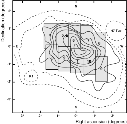
Figure 1: Position of the SMC fields (sm001 to sm010) on the de Vaucouleurs’ isophote map (de Vaucouleurs 1957). The star in field 5 indicates the position of the microlensing candidate. The isophote levels (inner to outer ones) are 21.4, 21.7, 22.0, 22.5, 22.8, 23.2, 23.9 ${\rm mag/arcsec^{2}}$ in red light ($\lambda=625$nm).

The fields were observed from July, 1996 to February, 1997 and again starting in July, 1997. During the 1996-97 season, from 60 to 120 usable images were taken of each field, giving a sampling time of one point every 2-4 days on average. Exposure times varied from 5 min in the central fields to 15 min in the outermost fields.

The DLT tapes produced in Chile are shipped to the CCPN (IN2P3 computing center, CNRS) in Lyons, France, where data processing occurs. For each of the fields, a template image is first constructed by adding together 10 exposures of good quality, each re-sampled by a factor of 0.7. A reference star catalog is then built using the corrfind star finding algorithm (the stellar detection is done on a correlation image, obtained as described in section 3, page 3). For each subsequent image, after geometrical alignment to the template catalog, each star identified on the reference catalog is fitted together with neighboring stars, using a PSF determined on bright isolated stars and imposing the position from the reference catalog. A relative photometric alignment is then performed, assuming most stars do not vary. Photometric errors are computed for each measurement, assuming again that most stars are stable, and parameterized as a function of star brightness and image sequence number. Photometric accuracy is in the $8-20\%$ range at magnitude $V\sim 20$ (depending on image quality), and of the order of $2\%$ for bright stars ($V\sim 17$). The number of reconstructed stars varies from $8\times 10^{5}{\rm\>deg}^{-2}$ in the densest region (where errors are dominated by crowding) to $4\times 10^{5}{\rm\>deg}^{-2}$ in the outer regions (where errors are dominated by signal-to-noise). The photometry is described in more details in (Ansari R. 1996b ).

3 Data analysis

The 5.3 million light curves are subjected to a series of selection criteria and rejection cuts (globally called “cuts”) to isolate microlensing candidates (Palanque-Delabrouille 1997). The first three (1–3) make use of the expected general characteristics of microlensing candidates: single variations on otherwise constant light curves, which coincide in time for data taken in both colors. The next two cuts (4 and 5) are designed to reject a known background of variable stars, while the last two (6 and 7) improve the signal-to-noise of the set of selected candidates. The criteria were sufficiently loose not to reject events affected by blending or by the finite size of the source, or events involving multiple lenses or sources. We define a positive (negative) fluctuation as a series of data points that (i) starts by one point deviating by at least $1\sigma$ from the base flux, (ii) stops with at least three consecutive points below ${\rm base\>flux}+1\sigma$ (above ${\rm base\>flux}-1\sigma$) and (iii) contains at least 4 points above ${\rm base\>flux}+1\sigma$ (below ${\rm base\>flux}-1\sigma$). The significance $LP$ of a given variation is defined as the negative of the logarithm of the product, over the data points it contains, of the probability that each point deviates from the base flux by more than the observed fluctuation ($x_{i}$ is the deviation of the point taken at time $t_{i}$, in $\sigma$’s, $N$ is the number of points within the fluctuation):

$$LP=-\sum_{i=1}^{i=N}\log\left(\frac{1}{2}\>{\rm Erfc}\left(\frac{x_{i}}{\sqrt{2}}\right)\right)$$ (1)

We order the fluctuations along a light curve by decreasing significance. The cuts of the analysis are described hereafter:

• 1: The main fluctuation detected in the red and blue light curves should be both positive and occur simultaneously: if I is the time interval during which the data are more than $1\sigma$ away from the base flux, we require $({\rm I_{red}}\cap{\rm I_{blue}})/({\rm I_{red}}\cup{\rm I_{blue}})>20\%$.

• 2: To reject flat light curves with only statistical fluctuations, we require that on a given light curve
  $LP({\rm 2^{nd}\>most\>significant\>fluct.})\>/\>LP({\rm main\>fluct.})<0.35$
  in both colors.

• 3: We require that $LP(\rm main\;fluct.)>30$ in both colors.

• 4: To exclude short period variable stars which exhibit scattered light curves, we require that the RMS of the distribution of the deviation, in $\sigma$’s, of each flux measurement from the linear interpolation between its two neighboring data points be smaller than 2.5.

• 5: We remove two under-populated regions of the color-magnitude diagram (see figure 2) that contain a large fraction of variable stars ($\beta$ Cephei, RV Tauri variables, semi-regular giant variables and Mira Ceti stars), defined by (flux $F$ given for the EROS2 filters — $R$ for red and $B$ for blue — normalized to an exposure time of 300 s):
  $\log(F_{R}/F_{B})<-0.20$ and $\log(F_{R})>4.5$
  $\log(F_{R}/F_{B})>+0.07$ and $\log(F_{R})>2.7$

  Figure 2: Cut on color-magnitude diagram, here shown for field sm001. The dotted lines delimit the rejected areas. The dots correspond to all the light curves in the field, the star markers are the remaining objects for this field, after cuts 1 through 4.

• 6: We remove events with low signal-to-noise by requiring a significant improvement of a microlensing fit (ml) over a constant flux fit (cst), i.e. that
  $[\chi^{2}({\rm cst})-\chi^{2}({\rm ml})]/[\chi^{2}({\rm ml})/{\rm d.o.f.}]>150$
  where d.o.f. is the number of degrees of freedom.

• 7: We require that the maximum magnification in the microlensing fit be greater than 1.40.

The tuning of each cut and the estimate of the efficiency of the analysis is done with Monte Carlo simulated light curves. To ensure similar photometric dispersion on simulated events and on the data, the events are added to real  light curves. The microlensing parameters are drawn uniformly in the following intervals: time of maximum magnification $t_{0}\in[t_{\rm first}-150,t_{\rm last}+150]$ days, impact parameter normalized to the Einstein radius $u_{0}\in[0,2]$ and time-scale (Einstein radius crossing time) $\Delta t\in[0,150]$ days. We correct for blending statistically, using a study of the typical flux distribution of the source stars which contribute to the flux of a reconstructed star, depending on its position in the color-magnitude diagram.

	Number of	Fraction of remaining
Cut description	stars	stars removed by cut
	remaining	Data	Simulation
Stars analyzed	5,277,858	-	-
1: Simultaneity	125,071	98%	80%
2: Uniqueness	36,032	71%	13%
3: Significance	4,022	89%	13%
4: Stability	1,214	70%	16%
5: HR diagram	463	62%	6%
6: Microlensing fit	48	89%	20%
7: Magnification	10	76%	16%

Table 1: Impact of each cut on data and simulated events. Each fraction for cut $n$ refers to the stars remaining after cut $(n-1)$.

Table 1 summarizes the impact of the cuts. The first requirement removes 98% of the data light curves which are just flat light curves. It also removes a large fraction of the simulated events of too low amplitude (large impact parameter) or short-duration events peaking well outside the observational period $[t_{\rm first},t_{\rm last}]$. The other cuts remove a large fraction of remaining data light curves (background) while leaving, in general, at least 75% of the simulated light curves.

The efficiency of the analysis (cuts 1 through 7) for detecting real microlensing events is determined from the set of simulated microlensing events, taking into account the effect of blending. The efficiencies (in %) normalized to an impact parameter $u_{0}<1$ and an observing period $T_{\rm obs}$ of one year are summarized in table 2 for various Einstein radius crossing times $\Delta t$ (in days).

$\Delta t$	7	22	37	52	67	82	97	112	127
$\epsilon(\Delta t)$	8	16	20	22	24	27	28	29	30

$\Delta t$	150	300	500	1000	1500	2000
$\epsilon(\Delta t)$	29	28	27	24	19	17

Table 2: Efficiency (in %) of the analysis (cuts 1–7) for various time-scales $\Delta t$ (in days), normalized to $u_{0}<1$ and $T_{\rm obs}=1{\rm\>yr}$. We monitor $N_{\rm obs}=5.3\times 10^{6}$ stars. The efficiency values for $\Delta t>150$ days are obtained by simulating events of duration $\Delta t$ over a period $[t_{\rm first}-\Delta t,t_{\rm last}+\Delta t]$ days.

4 Study of the candidates

Of the 5.3 million light curves, ten events passed all cuts and were inspected individually. Scanning of Monte Carlo events indicates that a negligible number of remaining candidates would be rejected by visual inspection. Three of the ten candidates exhibit new variations on their light curve when adding the first data from the second year survey, and are probably recurrent variable stars. Another event has its light curve affected by the appearance of a neighboring object which is below our detection threshold in the template image, but becomes very bright for a period of about 60 days. The object could be a nova or even a microlensing on an unresolved star. This analysis, however, uses only stars identified on the template image, so the light curve must be rejected. Four more events have light curves incompatible with microlensing and are probably due to other physical processes (one of them is a nova in the SMC (Alcock et al. 1997a )). Another event exhibits a very chromatic variation ($A_{R}=1.7$ and $A_{B}=1.2$). If this were due to blending (i.e. when both the magnified star and an undetected star contribute to the total reconstructed flux), the star undergoing the magnification would be of similar brightness as clump giant stars but redder than clump giants by about 1.2 magnitude. It could not belong to the SMC and a microlensing interpretation of this event is thus unrealistic. Thus, 9 out of the 10 candidates are rejected by this inspection.

The remaining light curve is shown in figure 3. It fits well the standard microlensing hypothesis with an Einstein radius crossing time of 104 days, a maximum magnification of 2.1 (impact parameter $u_{0}=0.53$) occurring on January 11, 1997 and $\chi^{2}/{\rm d.o.f.}=268/161=1.7$.

Figure 3: Light curve of microlensing candidate SMC #1, with a standard microlensing fit (combined for the red and blue light curves) superimposed, with no blending assumed. Time is in days since Jan. 0, 1990 (Julian date 2,447,891.5).

The source star is located at $\alpha=01^{\rm h}00^{\prime}5.64^{\prime\prime}$ and $\delta=-72^{\circ}15^{\prime}2.41^{\prime\prime}$ (J2000), and is labeled U0150_00676152 in the USNO star catalog. The magnitude of the source star given in the catalog is $R\simeq 18$. This microlensing candidate was also reported by the MACHO collaboration and exhibited no variation during 3 years preceding the upward excursion detected here (Alcock et al. 1997b ).

Because of the high stellar density of the fields monitored in microlensing surveys, the flux of each reconstructed star generally results from the superposition of the fluxes of many source stars. We thus introduce two additional parameters in the fit : the contribution $c_{\rm\,bl}$ in both colors of the base flux of the magnified star ($f_{\rm star}$) to the total base flux recovered ($f_{\rm star}+f_{\rm blend}$):

$$c_{\rm\,bl}\equiv\frac{f_{\rm star}}{f_{\rm star}+f_{\rm blend}}=\frac{A_{\rm reconstructed}-1}{A_{\rm real}-1}$$ (2)

The blending coefficient $c_{\rm bl}$ is unity when there is no blending and $c_{\rm bl}\rightarrow 0$ in the limit where the magnified star does not contribute at all to the total recovered baseline flux. Allowing for blending does not significantly improve the fit, but changes the best estimate values of the fit parameters, as shown in table 3. The errors on the blending coefficients are of 20%.

Fit	$u_{0}$	$t_{0}$	$\Delta t$	$c_{\rm\,bl}\;R$	$c_{\rm\,bl}\;B$	$\chi^{2}/{\rm d.o.f.}$
Red	$0.53$	$2567$	$100$	-	-	164/94
Blue	$0.54$	$2567$	$103$	-	-	99/64
Combined	$0.53$	$2567$	$104$	-	-	268/161
Blended	$0.41$	$2567$	$123$	$0.71$	$0.71$	266/159

Table 3: Results of microlensing fits to the SMC candidate. $t_{0}$ is the time of maximum magnification and $\Delta t$ the Einstein radius crossing time, both given in days.

The magnified source star would then have $\log(f_{R})=3.90$ and $\log(f_{R}/f_{B})=-0.38$ while the blend companion would have $\log(f_{R})=3.53$ and $\log(f_{R}/f_{B})=-0.39$. This amount of blending is in agreement with the estimate given by the MACHO collaboration.

The blending hypothesis is strengthened by the observation of a slight shift in the position of the centroid of the reconstructed star as the magnification occurs: $(\Delta\delta\simeq 0.072{\rm\;arcsec},\>\Delta\alpha\simeq-0.090{\rm\;arcsec})$. This shift can be caused by the displacement of the barycenter of the positions (weighted by the flux) of the two components of the blend. The direction of this displacement (slope $|\Delta\alpha/\Delta\delta|$ of $1.25$) is compatible with the direction of the apparent elongation of the source star ($\Delta\delta\simeq-0.95{\rm\;arcsec},\>\Delta\alpha\simeq 1.26{\rm\;arcsec}$ i.e. a slope of 1.3) in the image of the correlation coefficients between a Gaussian Point Spread Function (PSF) and the template image (the correlation image is shown in figure 4, right):

$${\rm coeff.}=\frac{{\rm covariance\,}(PSF,Image)}{\sqrt{{\rm variance\,}(PSF)}\;\sqrt{{\rm variance\,}(Image)}}$$ (3)

The correlation is calculated over a radius of $1.6\sigma$, where the $\sigma$ of the PSF is related to the seeing by ${\rm seeing}=2\sqrt{2\ln 2}\,\sigma$. The reconstructed source star might therefore consist of two components, located approximately 1.5 arcsec apart. Both the template image and the correlation image of an $8{\rm\;arcsec\times 8\;arcsec}$ area around the candidate are shown in figure 4. The pixel size on the template image is 0.42 arcsec, that on the correlation image is 0.21 arcsec.

Figure 4: Template image and correlation image around the candidate. North is to the left, East is up.

Note the clear improvement in stellar separation (and in stellar detection, as evidenced with the leftmost star) in the correlation image as compared to the template image, which allows us to infer the existence of a blend companion and estimate its position. Requiring on the template image (figure 4, left) the existence of two source stars located along the observed position angle (instead of a single star recovered as with the standard star finding algorithm), we can estimate the flux ratio of the two stars. In the best fit, the light is split with the ratio 70% to 30% between the two blended components. This independent method thus gives a result consistent with that of the microlensing fit.

As can be seen in figure 3, the measured luminosities exhibit an abnormally high scatter in the two colors. Correspondingly, the $\chi^{2}/{\rm d.o.f.}$ (266/159 in Table 2) has a low probability, of order $10^{-5}$. As a significant correlation is observed between the residuals of the fit in both colors (99.5% CL), a search for periodicity was performed on these residuals. The most likely period was found at $P=5.124$ days, with a false detection probability of $2.\>10^{-6}$ (other periods, aliases of $P$, are less probable, though not excluded). Figure 5 shows the residuals light curve, folded to $P=5.124$ days. About 1.5% of the main sequence stars of similar brightness have a light curve which exhibits a periodic modulation of at least a $\sim$2% amplitude.

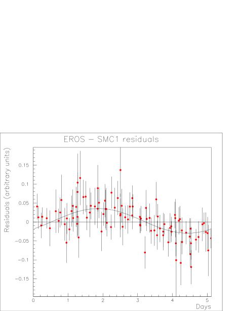
Figure 5: Light curve of the residuals in red, folded to $P=5.124$ days.

We then repeated the microlensing fits of table 2, including a sinusoidal modulation with three additional free parameters: period, phase and amplitude of the modulation (identical for both colors). Results of the fit are given in table 4. The fits give almost identical results for $u_{0},t_{0},\Delta t$ and blending factors as those in table 2 (respectively 0.42, 2568., 123. and 0.74). Of course, the modulation can affect either the amplified component, or the blended companion. The results of the fits favor the first possibility, though only at the $2.5\sigma$ level. We expect that the data reported by the MACHO collaboration (Alcock et al., 1997b) have enough statistical power to discriminate between these two possibilities. We remark that the $\chi^{2}$ of the fits including a modulation term are satisfactory, indicating accurate modeling of errors.

Star modulated	$A_{\rm mod.}$ (in %)	$P_{\rm mod.}$ (in days)	$\chi^{2}/{\rm d.o.f.}$
magnified star	$2.9\pm 0.5$	$5.128\pm 0.004$	157/156
blend companion	$11.\pm 7.$	$5.128\pm 0.004$	163/156

Table 4: Result of microlensing fit + sinusoidal modulation on either component of the blend. $A_{\rm mod.}$ is the amplitude of the modulation normalized to the unamplified stellar flux, and $P_{\rm mod.}$ the period.

Figure 6 illustrates the position of the candidate reconstructed star in the color-magnitude diagram of the surrounding region (star marker), as well as that of the two components of the blend (circles). They all lie on the main sequence.

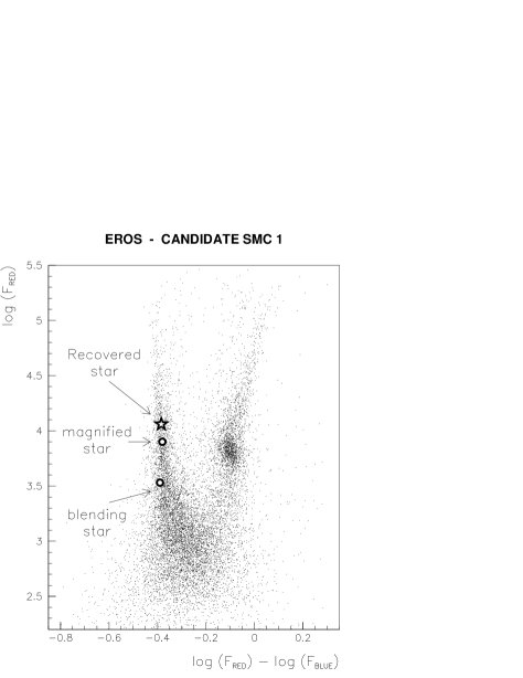
Figure 6: Color-magnitude diagram of the field surrounding the microlensing candidate. The exposure time on this field was 480 s and is here renormalized to 300 s for comparison with figure 2. The recovered star is plotted with a star marker, the components of the blend with circles.

5 Estimate of optical depth and lens mass

The optical depth is the instantaneous probability that a given source star be magnified by more than a factor of 1.34. It can be estimated as

$$\tau=\frac{1}{N_{\rm obs}T_{\rm obs}}\>\frac{\pi}{2}\sum_{\rm events}\frac{\Delta t}{\epsilon(\Delta t)}$$ (4)

where $\epsilon(\Delta t)$ is the detection efficiency given in table 2, $T_{\rm obs}=1$ year and $N_{\rm obs}=5.3\,10^{6}$ stars. With the characteristics of the single event described above, this yields (fit with blending):

$$\tau\simeq 3.3\times 10^{-7}$$ (5)

i.e. about 50% of the optical depth predicted by a “standard” isothermal and isotropic spherical halo fully comprised of compact objects (cf section 5). It is consistent with that measured toward the Large Magellanic Cloud (Alcock et al. 1997c , see also Ansari et al. 1996a).

Assuming a standard halo model with a mass fraction $f$ composed of dark compact objects having a single mass $M$, a likelihood analysis allows us to estimate the most probable mass of the deflector generating the observed event. The likelihood is the product of the Poisson probability of detecting $N_{\rm evt}$ events when expecting $f\,N_{M}$, by the probability of observing the time-scales $(\Delta t_{1},..\,,\Delta t_{\rm evt})$. We calculate likelihood contours in the $(\log(M),f)$ plane using a Bayesian method with a uniform prior probability density in $f$ and in $\log(M)$ (i.e. equal probability per decade of mass). They are shown in figure 7.

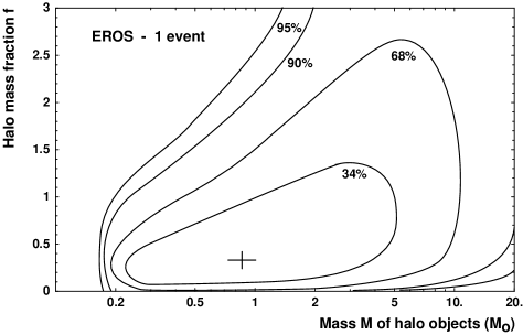
Figure 7: Likelihood contours with one microlensing candidate for a standard halo model. The cross marks the peak of the 2-D distribution (solution with blending).

We integrate over $f$ to obtain the 1-D likelihood for the mass of the deflector. This yields the most probable mass of the Halo deflector, given with $1\sigma$ error bars:

$$M=2.6^{+8.2}_{-2.3}{\rm\;M_{\odot}}$$ (6)

More statistics is obviously required to constrain the mass of halo deflectors.

6 Expected number of Halo events — model dependence

We studied a wide range of disk-halo models. Table 5 summarizes their characteristics. The rotation velocity at the Sun predicted by these models is always within the observational range: $V_{\rm Tot}({\rm R_{\odot}})\simeq 200{\rm\>km/s}$ (Merrifield 1992), or $V_{\rm Tot}({\rm R_{\odot}})=220\pm 15{\rm\>km/s}$ (Binney and Tremaine 1987). The optical depth is independent of the mass of the deflectors; the event rate is given assuming that all deflectors in the halo have a single mass equal to $1{\rm\;M_{\odot}}$. To obtain the predicted value of the event rate for other masses, one only needs to scale by $\eta_{M}$, the integral of the mass dependence of the event rate times $f_{M}(M)$, the normalized mass distribution:

$$\eta_{M}=\int f_{M}(M)\frac{1}{\sqrt{M/{\rm\;M_{\odot}}}}\>dM$$ (7)

This simplifies to $(M/{\rm\;M_{\odot}})^{-1/2}$ for a Dirac distribution peaked at $M$.

MODEL	1	2a	2b	3	4	5
$\Sigma_{0}\>({\rm\;M}_{\odot}/{\rm pc}^{2})$	50	50	100	50	50	80
$\rho_{\odot}\>({\rm\;M}_{\odot}/{\rm pc}^{3})$	.008	.008	.003	.014	.00	.005
$\beta$	-	0	0	0	0.2	0
$q$	-	1	1	0.71	1	1
$M({60\>\rm kpc})$	5.1	1.9	0.7	2.0	1.2	2.2
$V_{\rm Tot}({\rm R_{\odot}})\>({\rm km/s})$	192	202	221	205	199	219
$V_{\rm Halo}(50{\rm\>kpc})$	189	164	100	169	134	163
$V_{\rm Tot}(50{\rm\>kpc})$	199	176	133	180	148	182
$\tau\>(10^{-7})$	6.8	5.7	2.1	3.9	4.2	3.8
$\Gamma\>({\rm 10^{-7}\,yr^{-1}})$	22.8	17.8	5.4	14.2	12.6	9.1

Table 5: Description of the Galaxy models. We give the mass $M$ of the halos out to the SMC (in units of $10^{11}{\rm\;M}_{\odot}$), the rotation velocities (in km/s), the optical depth $\tau$ and the event rate $\Gamma$ for $1{\rm M_{\odot}}$ deflectors (with a 100% efficiency). $\Sigma_{0}$ is the central column density, $\rho_{\odot}$ the local halo density at the Sun, $\beta$ is proportional to the asymptotic slope of the rotation curve and $q$ is the flattening ratio of the halo.

Model 1 is the “standard” halo model: an isotropic and isothermal spherical halo, with a mass distribution given in spherical coordinates by (Caldwell and Coulson 1981):

$$\rho(r)=\rho_{\odot}\frac{R_{\odot}^{2}+R_{c}^{2}}{r^{2}+R_{c}^{2}}$$ (8)

where $R_{c}=5$ kpc is the Halo “core radius” and $R_{\odot}=8.5$ kpc is the distance from the Sun to the Galactic Center. Model 2a is the equivalent power-law model (Evans, 1993). Model 2b has a maximal disk ($\Sigma_{0}=100{\rm\;M}_{\odot}/{\rm pc}^{2}$) and a very light halo, model 5 intermediate disk and halo. Model 3 has a flattened E6 halo (axis ratio $q=0.71$) and model 4 a decreasing rotation curve ($\beta=0.2$ where $\beta$ is proportional to the logarithm of the asymptotic slope). Models 2–5 are all power-law halo models, with self-consistent mass and velocity distributions. For each of these, we derive the expected number of events versus the mass $M$ of the objects in the Halo (assuming a Dirac mass distribution) and compare with the observations (cf figure 8).

Figure 8: Expected number of events for the models described in the text, including the experimental efficiency.

Whatever the halo model considered, the sole event we observed, if caused by a deflector in the halo of our Galaxy, corresponds to at least 40% of the total optical depth expected for $f=1$. This is a very small number statistics, however.

7 Parallax analysis

The very long time-scale of the observed event suggests that it could show measurable distortions in its light curve due to the motion of the Earth around the Sun, (the parallax effect: Gould 1992), provided that the Einstein radius projected onto the plane of the Earth is not much larger than the Earth orbital radius. The first detection of parallax in a gravitational microlensing event was observed by Alcock et al. (1995). The natural parameter to measure the strength of parallax is the semi major axis of the Earth orbit, $R_{O}$, in units of the projected Einstein radius: $\delta u=R_{O}(1-x)/R_{E}$ where $x=D_{d}/D_{s}$, with $D_{d}$ the distance from the observer to the deflector and $D_{s}$ the distance to the source.

No evidence for distortion due to parallax is detectable on the light curve, implying either a very massive deflector with a very large Einstein radius, or a deflector near the source. Because our results for the standard and blended fits (see table 3) agree well with those obtained by the MACHO collaboration with a 3 year baseline (Alcock et al. 1997b), we will fix the level of the baseline flux to that obtained previously with the blended fit, to perform parallax fits. We fit simultaneously the red and blue light curves allowing for parallax and for the periodic modulation described in section 3. Assuming a blending coefficient $c_{\rm bl}=0.74$, our data allows us to exclude, at the 95% CL, that $\delta u>0.054$. This yields a lower bound on both the projected transverse velocity of the deflector:

$$\tilde{v}=R_{O}/(\Delta t\>\delta u)=v_{t}/(1-x)>270{\rm\;km/s,}$$ (9)

and on the projected Einstein radius:

$$\tilde{R}_{E}=\Delta t\>\tilde{v}=R_{E}/(1-x)>18{\rm\;AU.}$$ (10)

We can thus write:

$$(\tilde{R}_{E})^{2}=\frac{4GM}{c^{2}}\times D_{s}\frac{x}{1-x}>(18{\rm\>AU})^{2}$$ (11)

$$\Longrightarrow\frac{M}{\rm M_{\odot}}\times\frac{x}{1-x}>0.7$$ (12)

The high projected transverse velocity definitely excludes the possibility that the deflector is in the disk of the Milky Way, where the typical velocity dispersion is $\sim 30-40$km/s (Binney and Tremaine 1987). Moreover, a disk lens (i.e. $x<1/100$) generating this event would have a mass $M>70{\rm\;M_{\odot}}$! For a deflector in the halo, $x<2/3$ at the 95% confidence level (for a standard halo) which requires the mass of the deflector $M$ to be at least $0.3{\rm\;M_{\odot}}$, while for a deflector in the SMC, if $1-x\simeq 1/10$, the mass of the lens would be $M\simeq 0.07{\rm\;M_{\odot}}$. This is illustrated in figure 10.

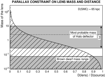
Figure 9: Relation mass-distance of the deflector, from the parallax analysis. Only the region above the curve is allowed. The top gray area is the $1\sigma$ most probable mass of a Halo deflector (see section 4).

Figure 10: Degeneracy valleys between parallax and blending effects. Top plot: blending coefficient compensating the effect of parallax. Bottom plot: angle (in degrees) between the directions of the line of sight and deflector velocities compensating the effect of parallax. Full and empty markers correspond to the same $\chi^{2}/{\rm d.o.f.}$, but the first set tends to an angle of 180 degrees, while the second tends to an angle of 0. The four sets of markers correspond to the four possible relative motions of the Earth and the deflector.

It is possible for some parallax distortions to be largely cancelled out by blending effects. However, blending distortions of light curves are always symmetric about the point of highest magnification, while this is not the case, in general, of parallax distortions. It is only true when the velocity of the deflector is parallel or anti-parallel to the velocity of the Earth around the Sun at the moment of highest magnification. Figure 10 illustrates the amount of blending required to compensate the effect of an increasing parallax while remaining compatible with the observed light curve. All the points plotted yield a $\chi^{2}/{\rm d.o.f.}$ for the fit within $1\sigma$ of the minimum value (157/158). Note the two minima regions in the planes shown in the figure, one around an angle of 180 degrees between the projected velocities of the Earth and of the deflector (full markers), while the other (empty markers) corresponds to a null angle. The shaded area delimits blending coefficients greater than unity, which is not physical. As shown in figure 10, $\delta u$ could be larger than 0.054, but only in the unlikely case of alignment of velocities. We built a likelihood based on the fit with parallax, blending and a modulation on the magnified star, taking into account the probability that the alignment of the Earth and deflector velocities were parallel or anti-parallel. This yields the 95% CL upper limit $\delta u<0.06$ (which requires a blending coefficient $c_{\rm bl}=0.45$). The projected velocity is then constrained to be at least 190 km/s and equation 12 becomes $\frac{M}{\rm M_{\odot}}\times\frac{x}{1-x}>0.5$.

8 Discussion — SMC self lensing

If the deflector belongs to the Halo of our Galaxy, it is expected to have a mass greater than a third of a solar mass (see sections 5 and 7); and yet to be dim enough to avoid direct detection, it could only be a white dwarf, a neutron star or a black hole. It is also possible, however, that both the lensing object and the source star belong to the SMC, in which case the deflector would have a much smaller mass.

Let us estimate the optical depth for SMC self-lensing. Various authors have suggested that the SMC is quite elongated along the line-of-sight, with a depth varying from a few kpc (the tidal radius of the SMC is of the order of 4 kpc) to as much as 20 kpc, depending on the region under study (Hatzidimitriou and Hawkins 1989, Caldwell and Coulson 1986, Mathewson et al. 1986). We will approximate the SMC density profile by a prolate ellipsoid:

$$\rho=\frac{\Sigma_{0}}{2h}\>e^{-|z|/h}\>e^{-r/r_{d}}$$ (13)

where $z$ is along the line-of-sight and $r$ is transverse to the line-of-sight. The depth $h$ will be a free parameter, allowed to vary between 2.5 and 7.5 kpc. Fitting for instance the Mathewson et al. Cepheid data (Mathewson et al. 1986) in the bar of the SMC with the above density distribution gives $h\sim 5.8\pm 1.2$ kpc (assuming Poissonian statistics on the Cepheid counts). The other parameters are estimated from the surface-brightness map of de Vaucouleurs (see figure 1) using the identity:

$$R=26.1{\rm\>mag/arcsec^{2}}\Longleftrightarrow 1{{\rm\>L_{\odot}/pc^{2}}}$$ (14)

derived from $M_{V}=4.83-2.5\log(L_{V}/{\rm L}_{\odot,V})$, $M_{R}-M_{V}=-0.35$ for the Sun. Plotting the isophote levels $R$ as a function of the mean distance of each isophote to the optical center of the SMC (see figure 11), we can derive the central surface brightness: $R_{0}=20.7{\rm\>mag/arcsec^{2}}$. The slope of the fit yields the value of the radial scale length: $r_{d}=0.54$ kpc.

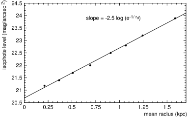
Figure 11: Isophote level (from the de Vaucouleurs’ map) vs. mean distance to optical center of the SMC.

Assuming a mass-to-light ratio of $\sim 3{\rm\;M_{\odot}/L_{\odot}}$, this gives a central surface density $\Sigma_{0}\simeq 400{\rm\;M_{\odot}pc^{-2}}$ and a total SMC mass of $\sim 1\times 10^{9}{\rm\;M_{\odot}}$, compatible with that estimated from the mass of the LMC considering that the SMC is only $\sim 20\%$ as bright. We denote as $z_{d}$ and $z_{s}$ the positions of the deflector and the source, both in the SMC, with origin taken at the center of the SMC.

Assuming the same spatial distribution for the source stars and the lenses, the optical depth for SMC self-lensing is given by

$$\tau=\frac{\int\tau(z_{s})\;\frac{\rho(z_{s})}{M}r\;dr\;d\theta\;dz_{s}}{\int\frac{\rho(z_{s})}{M}r\;dr\;d\theta\;dz_{s}}$$ (15)

where $\tau(z_{s})$ is the usual optical depth due to source stars all at a distance $z_{s}$ and deflectors at $z_{d}$ contained in the elementary volume $r\>dr\>d\theta\>dz_{d}$:

$$\tau(z_{s})=\int_{-\infty}^{z_{s}}\frac{\rho(z_{d})}{M}\;dz_{d}\;\pi\frac{4GM}{c^{2}}\frac{(D_{s}+z_{d})(z_{s}-z_{d})}{(D_{s}+z_{s})}.$$ (16)

For $h=2.5$, 5.0 or 7.5 kpc, this yields optical depths $\tau=1.0\;10^{-7}$, $1.7\;10^{-7}$ or $1.8\;10^{-7}$ respectively. Considering the very limited statistics we have, this optical depth is consistent with the observations.

Let us also consider the expected typical time-scales of SMC-SMC microlensing events. The velocity dispersion in the SMC is $<\!\sigma\!>\>\sim$ 30 km/s (Hatzidimitriou et al. 1997, Suntzeff et al. 1986), so the estimated mass $M$ of the deflector causing the observed event ($\Delta t=123$ days) could be greatly reduced compared to that of a halo deflector. On average, we have:

$$\frac{M}{\rm M_{\odot}}\times x(1-x)\simeq 0.0088$$ (17)

Thus, if the deflector is 5 kpc (resp. 2.5 kpc) from the source, we have $M\sim 0.1{\rm\;M_{\odot}}$ (resp. $0.2{\rm\;M_{\odot}}$).

As more data are accumulated, we expect SMC-SMC events to be highly concentrated in high density regions of the Cloud (see figure 1), unlike Halo events which should be distributed like the SMC stars over the sky. In addition, they should not have measurable parallax distortions. These criteria will help distinguish between the two possibilities.

9 Conclusion

We have presented here the result of a one-year survey toward the Small Magellanic Cloud with EROS2. One star has a light curve that is best interpreted as due to microlensing with an Einstein radius crossing time of 123 days when allowing for blending, with 70% of the total baseline flux contributed by the star being lensed. The light curve exhibits a 2.5% modulation with a period $P\simeq 5.12$ days. The optical depth estimated from this event is $\sim 3.3\times 10^{-7}$, to be compared with $\tau=6.8\times 10^{-7}$ for a spherical isothermal halo containing only such objects. The most probable mass of the deflector (if it is in the Halo) would be $M=2.6^{+8.2}_{-2.3}{\rm\;M_{\odot}}$. If we interpret this event as due to a deflector in the SMC, the expected optical depth is $\tau\simeq 1.7\times 10^{-7}$ for a depth scale-length of the SMC of 5 kpc, and the mass of the deflector would be reduced to about $0.1{\rm\;M_{\odot}}$. Given the very small statistics, the SMC interpretation seems possible. Furthermore, we observe no distortion on the light curve due to the varying velocity of the Earth on its orbit around the Sun (parallax), although some would have been expected for such a long duration event, unless the deflector were either very heavy or near the source. This further supports the SMC lens interpretation.

Further observations will help discriminate Halo from Cloud deflectors. In particular, because the velocity dispersions in the LMC and the SMC differ by almost a factor of 2, the observation of a significant trend for longer time-scale events toward the SMC than toward the LMC would be a clear signature of events dominated by SMC or LMC self-lensing.