Cosmic Rays: Studying the Origin

1 Introduction

Results from many experiments provide continuously improving knowledge about cosmic rays (CR). To interpret this knowledge it is necessary to combine information from various areas of astronomy, particle physics, plasma physics, geophysics and others. The phenomenon of CR relates to astronomy since CR come from outside the Earth, most of them from outside the Solar System. CR are detected due to their interaction with matter and the detectors are the same as used in particle physics. CR are the phenomenon of Nature. All experiments are passive. This paper describes in some details author’s contribution to interpretation of experimental results on the background of general trends of research in this area. Particular results are from experiments which sometimes based on very different principles, from satellite detectors to deep underground detectors, all giving contribution to cosmic ray studies.

Many years after the discovery of cosmic rays their origin is still unknown. There are problems with naming the sources (if they are), as well as with naming the mechanism of particle acceleration. It is accepted that acceleration is an ordinary (astro)physical process, i.e. with the well known physical basic phenomena playing the crucial role, but placed in not understood, and therefore “complicated”, time–space scenario. To dramatize the problem a little, let us notice that the very sophisticated, man built accelerators can accelerate protons to the energy about 1000 GeV (at the beginning of 1997), whereas the measured flux of CR protons above energy 100,000 GeV is equal to about 2$\cdot$10^-5 particles per (m${}^{2}\cdot{\rm sr}\cdot{\rm sec}$) (i.e. 3$\cdot$10¹⁰ such protons are hitting the Earth’s atmosphere every second) and more than 1000 of the most energetic CR of energies above 10,000,000,000 GeV (10¹⁰ GeV) have been registered.

Let us accept following definition of primary cosmic rays as energetic particles of nonthermal origin, present in the space outside the Earth atmosphere. They are protons and other nuclei, electrons, gamma photons, positrons, antiprotons and neutrinos.

Different components have different abundances, different energy spectra, different ability of being measured. There is no evidence that all of them have common sources. We can make relations between abundances of some of them (e.g. the bulk of antiprotons being secondary particles from CR protons and nuclei collisions with the interstellar medium [89, Szabelski et al., 1980]). The only common features are their relatively high energy and the problem with the explanation of their origin.
There are many attempts to explain the mechanism of CR acceleration and I would like to mention the shock wave acceleration mechanism which has many achievements and is very fashionable in the recent years. Since there is no observational evidence pointing exclusively to this mechanism, as well as there are problems with acceleration efficiency and explanation of very high energy CR within this model, it looks reasonable to search for some other possible explanations of CR acceleration mechanisms as well.

Principally, it is necessary to refer to the experimental studies of CR origin and acceleration. The most important are different measurements of CR and related events. We know the energy spectra of various components, absolute or relative abundances of components, anisotropy, time variation etc. Thanks to them we have few models of CR ray propagation in our Galaxy, which provide some systematics to the bulk of information.

Before describing some detailed studies of CR origin it might be worth summarizing the problems in the simplified manner. This would provide a reference level for the role and importance of CR studies.

• Do observed CR originate within our Galaxy or are they of Universal origin ?

• Do they originate and are accelerated in the sources or are they of diffuse origin ?

• Is CR production uniform in time or intermittent ?

• Do all CR have the same origin or different components have principally different origin ?

• Are all CR accelerated by the same mechanism independent of their energy or by several different processes acting in limited energy regimes ?

• Is our position as “observers” typical in the Galaxy and is it typical in time ?

• Does the intensity of CR vary from place to place in our Galaxy and vary with time ?

Almost each of above questions requires an extended comment to explain its meaning, since a lot of work has been devoted to such problems. We know a lot at present time and, although the above list is not complete, many past time problems have been solved already.
However, the truly honest answer to each of above questions would be “YES or NO”, at present. Sometimes YES, sometimes NO, or “YES, but”, etc. Simply: there is no sufficient experimental evidence to provide the answer.

This work does not provide answers to above listed problems. It only addresses them.
The presented approach to study the CR origin shall not be treated as the unique, the best, nor even as the most promising. This is an approach. All other works are valuable, provided that their final results can be verified by experiment or observations.

The most complete information about cosmic ray physics can be found in the Proceedings of International Cosmic Ray Conferences; the last 24^th was held in Rome, Italy in August 1995, the 23^rd in Calgary, Canada in August 1993, the 22^nd in Dublin, Ireland in August 1991, the 21^st in Adelaide, Australia in January 1990, and the 20^th in Moscow, the USSR in August 1987.

The studies of cosmic ray origin can be systematized in the following way:

1. Search for CR “point sources”. There are experiments which are looking for enhancements of CR intensity around the well localized sources or enhancements of CR flux from such directions. The idea is simple: if there are CR “point sources” then the local intensity nearby the source is larger than average.
   The “only” problems are with observations. Paths of CR charged particles are bent in interstellar magnetic fields and incoming direction of observed CR particle does not point to the source. Therefore such studies are limited to

   1. gamma ray observations; $\gamma$–rays are CR secondaries from interactions of energetic particles with matter, and the interstellar medium is relatively transparent for them,

   2. neutrino astronomy; as above, but they are difficult to detect,

   3. very high energy CR observations; at extremely high energy the paths of CR protons are only slightly bent in galactic magnetic field, provided that the distance to the source is not too large,

   4. examining the possibility of high energy neutron flux from the nearby CR source,

   5. other astronomical methods; the very promising example is a comparison between the infra–red and radio emissivity in our Galaxy which allowed to point a number of non–thermal radio synchrotron emitting sources [37, Broadbent et al., 1989].

2. Studies of “CR sources” chemical composition. The direct measurements of CR mass composition were performed for CR energy below few hundred GeV. Results of local (at the Earth vicinity) measurements of absolute or relative mass composition of CR and the dependence of CR mass composition on energy are related to CR source chemistry, mechanism of acceleration and propagation properties. The research here reminds of solving the puzzle problem: some pieces fit each other, some others fit in another corner, but we are not able to make a whole picture, and, possibly, we do not have all the pieces yet.

   1. It is largely possible to measure the chemical composition of distant astronomical objects performing spectroscopic observation. Results of measurements of low energy CR mass composition are compared with observed star atmospheres to point out candidates for CR sources. The method has some “achievements”, e.g. correlation between the abundances of CR isotopes, the first ionization potential, and the chemistry of Wolf–Rayet stars atmosphere ([30, Blake and Dearborn, 1988]).

   2. The accurate measurements of chemical CR composition and its variability with energy was used to study the possibility of CR acceleration (or deceleration) during propagation [64, Giler et al., 1989].

   3. It is known that the CR intensity has a power law like energy spectrum, and its power index becomes smaller (steeper) by $\sim$ 0.3 near few times 10¹⁵ eV. There is a question of CR mass composition change in a region of power index change and above. The energy dependence of this changing is very important for studies of propagation properties, acceleration mechanisms and CR source problem.

   4. Observation of “secondary” CR particles energy spectra, i.e. particles originated in hadronic collisions of high energy CR with interstellar medium. These studies provide information on propagation properties of CR. The most important examples are studies of anti-proton flux, positron flux, ¹⁰Be, ⁵⁴Mn and few other long–life radioactive isotope fluxes, ³He, ²H and ³H fluxes.

3. Diffuse CR anisotropy measurements. Generally CR bombard uniformly the Earth’s atmosphere. The observed anisotropies are on the level lower than 10^-3. (Some anisotropies at low energy CR might be due to interplanetary propagation, and these are not considered here). The anisotropy studies might provide information on the nearby magnetic field configuration in the Galaxy.
   Anisotropy due to high energy photons from the Milky Way direction (from interactions of nuclear CR in the Galaxy) is predicted to be on the level of $\sim$5$\cdot$10^-5 [25, Berezinsky et al., 1993] and experimentally observed the first harmonic amplitude of (12.7$\pm$1.2)$\times$10^-4 or excess within $\pm$10^∘ in galactic latitude of 4$\cdot$10^-4 (1.5$\sigma$) [8, Alexeenko et al., 1993].

4. Time variability of diffuse CR intensity. Generally diffuse CR flux seems to be very stable in time. Observations of “cosmogenic nuclei” might provide information of CR variability over last $\sim$10⁵ years. Possible observation of large excess of CR flux about 3$\cdot$10⁴ years ago [74, Kocharov et al., 1990] might be interpreted as being due to shock acceleration mechanism during the passage of a supernova remnant shock wave at that time [88, Szabelska, Szabelski, Wolfendale, 1991].

Studies of some areas of cosmic ray origin problem are presented in this work. The selection reflects the author’s interest, and sometimes author’s contribution (made in collaborations).

• First experiments in gamma ray astrophysics are briefly presented. Then the state of $\gamma$–ray point sources investigation is presented. The next section is devoted to the studies of diffuse emission of $\gamma$–rays, i.e. due to interaction of cosmic rays with the interstellar matter. Author’s contribution is underlined. This is an area which develops very rapidly. Some knowledge we had $\sim$10 years ago is compared with the present situation.

• Studies of CR with energies 10¹⁴ – 10¹⁷ eV are presented in the Chapter 3. This is the area of extensive air shower (EAS) physics. Interpretation of experimental results requires large Monte–Carlo computer simulations. The main target of these studies are high energy nuclear interaction properties and CR mass composition end energy spectrum. Author’s selected research in this area relates to high energy muon groups as the promising method for studies of these problems. Results of computer simulations and experimental measurements are presented.

• Chapter 4 is devoted to the highest energy cosmic ray studies. The measurements of anisotropy are discussed. The experimental search of the highest energy CR sources is presented. Author’s contribution is underlined.

2 Gamma ray astrophysics

2.1 Introduction

In this section some studies of cosmic photons with energies above 30 MeV will be presented. These $\gamma$–rays are almost unabsorbed in the interstellar matter. Their directions point to the places where they were produced. The known production mechanisms require energetic particle (e⁺, e^- or nucleus). Therefore while studying these $\gamma$–rays one learns about cosmic rays at distant places.
All observations of $\gamma$–rays made so far show approximately (in large energy scale) power law decrease of $\gamma$–ray intensity with photon energy. The detector should have large enough area to be able to register higher energy cosmic $\gamma$–ray photons. The Earth atmosphere is not transparent to $\gamma$–rays. Observations outside the atmosphere are currently limited to $\gamma$–ray energy below $\sim$30 GeV. For satellite measurements a very efficient technique of discrimination of charged particle background has been developed, but energy measurement might require large and heavy devices.
Experimental measurements of higher energy $\gamma$–rays are located on the ground at mountain altitude. Energetic photon interacts in the atmosphere and produces electro–magnetic (E–M) cascade which consists of electrons, positrons and gammas (however, there is a chance of photo–production – $\gamma$–nucleus interaction with hadron products, in the first or subsequent interaction). E–M cascades produced by cosmic $\gamma$–rays of energy below 30 TeV (= 3$\cdot$10⁴ GeV = 3$\cdot$10¹³ eV) have no chance of being detected on the ground. However, some of e⁺ and e^- from these E–M cascades are faster than local phase velocity of light in the atmosphere and produce Cherenkov radiation which can be detected on the ground. Observation can be made at mountain altitudes during clear moonless nights. The lower $\gamma$–ray energy is limited by the strength of the Cherenkov light signal as compared with the dark–sky background (including stars in the field of view) and is equal to about 200 GeV at present. The upper limit is about 30 TeV due to statistics (falling intensity of $\gamma$–rays with energy).
$\gamma$–rays of energy above 10¹⁴ eV can produce E–M cascades which reach the ground at mountain altitudes. Therefore they can be observed by Extensive Air Shower (EAS) arrays.

Only satellite measurements can clearly discriminate photon observation from nucleus induced one in a single event. Thus the satellite measurements of $\gamma$–rays allow to make observations of wide angle structures on the sky, and allow to place the upper limits for $\gamma$–ray fluxes from low intensity directions, like diffuse extragalactic flux.

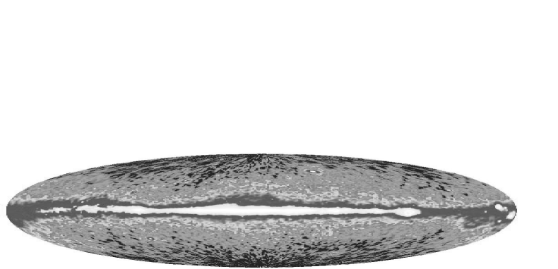
Figure 1: The contour map of $\gamma$–ray intensity (E${}_{\gamma}>$ 100 MeV) observed by the EGRET detector of Compton Gamma Ray Observatory. The map is in galactic coordinates, galactic centre in at the centre, the galactic longitude goes left from the centre (0${}^{\circ}\rightarrow$ 180^∘);
Crab (l_gal = 184.54^∘, b_gal = –5.88^∘) and Geminga (l_gal = 195.12^∘, b_gal = –4.27^∘) are clearly seen at the right of the figure, and Vela (l_gal = 263.52^∘, b_gal = –2.78^∘) is a white spot at a quarter right from the centre. The galactic plane is clearly seen. (Map obtained via computer network from NASA GSFC Science Support Center, April 1997)

2.1.1 Direct $\gamma$–ray measurements.

$\gamma$–rays with energies $\sim$30 – 1000 MeV were measured in the past by two experiments:

• SAS–II (Nov. 19, 1972 – June 8, 1973, due to “a failure of a capacitor on the input portion of the low–voltage power supply”) [59, Fichtel et al., 1975], [60, Fichtel et al., 1978] and

• COS B (1975 – 1982) [67, Hermsen, 1980], [84, Strong et al., 1987].

At present

• the EGRET instrument (April 25, 1991 – present time) [71, Kanbach et al., 1988], [93, Thompson et al., 1992] on the NASA Compton Gamma Ray Observatory (CGRO) measures $\gamma$–rays with energies $\sim$30 – $\sim$40000 MeV (however, the detection of one photon above 100 GeV has been reported in the Compton Observatory Science Report no 164 of the 2^nd of August 1994).

One can add to the list

• the unsuccessful French–Soviet–Polish experiment GAMMA–1 ([1, Agrinier et al., 1987]).

The principle of $\gamma$ detection is very similar in all these experiments. The basic idea for this detector is to register the electron and positron tracks, the pair produced inside the detector by the energetic photon. The multilayer spark chambers are used for this. $\gamma$–ray energy is measured in calorimeter as a sum of energy deposited by e⁺ and e^-. Thousands times larger proton flux is to be eliminated by the veto signal from shielding scintillation counters.
The angular resolution plays important role in data interpretation. For the photon direction determination the most important is the estimation of e⁺ and e^- tracks directions near to their place of origin. In about half of centimeter wide spark chambers of COS B experiment the e⁺e^- directions were estimated from spark position in subsequent chambers. There were problems with Coulomb scattering in spark chambers ‘horizontal’ walls.
The GAMMA–1 experiment had 3 cm wide spark chambers and it was possible (during calibration) to determine e⁺ and e^- directions within one gap (there were 3 scanning levels within each gap). Wide gaps of spark chambers required very high voltage supply and this created problems with electronic disturbance. Another problem is gas flushing of the spark chamber, and the gas storage limits the lifetime of the experiment. To improve angular resolution in the GAMMA–1 detector there were plans to use a special mask above the spark chambers to determine the entry point of $\gamma$–ray photon with still better precision (but this would decrease the effective area of detector nearly twice). The estimated accuracy of one $\gamma$–ray photon direction determination was $\sim$2^∘ at 100 MeV and $\sim$1^∘ at 500 MeV [3, Akimov et al., 1987] end energy resolution 40% – 60% [4, Akimov, Szabelski et al., 1990] (pre–flight calibration). GAMMA–1 was specially designed to search and observe $\gamma$–ray point sources, but the failure of high voltage power supply for spark chambers eliminated this experiment.
The EGRET detector has electronic read–out from spark chambers. The angular resolution of incident photon direction depends on its energy, position in the chamber and relative direction to detector’s optical axis. The in–flight calibration [93, Thompson et al., 1992] (from Crab observation) give folowing values of HWHM (half width at half maximum): 4.4^∘, 2.5^∘, 1.1^∘, 0.7^∘ and 0.4^∘ for energy ranges: 30 – 70 MeV, 70 – 150 MeV, 150 – 500 MeV, 500 – 2000 MeV and 2000 – 20000 MeV respectively. The corresponding values for the angular radius containing 67% of photons are: 8.4^∘, 5.6^∘, 3.1^∘, 1.6^∘ and 0.6^∘. The energy resolution is 20% – 30% (pre–flight calibration).

Subsequent experiments were

• bigger in size (geometric factor) to register larger number of gammas,

• longer lasting (with exception of GAMMA–1, which was scheduled for 1–2 years, only),

• more efficient: SAS–II has registered 12500 gammas, COS B – 209537, and the EGRET of CGRO is registering photons with a rate $\sim$0.01 Hz of effective time.

Together with other features each of the steps SAS–II $\rightarrow$ COS B $\rightarrow$ CGRO EGRET was a milestone of the $\gamma$–ray astrophysics.
Results of all–sky survey of the CGRO mission obtained by the EGRET detector and reduced to the intensity Aitoff plot is presented in the Figure 1.

2.1.2 Cherenkov light detectors of TeV range $\gamma$–rays.

$\gamma$–rays with energy around 1000 GeV ($\equiv$ 10¹² eV $\equiv$ 1 TeV) are measured by the ground based observation of Cherenkov light in the atmosphere. Energetic photon produces an electro–magnetic cascade of gammas, electrons and positrons in the atmosphere. The cascade originates high in the atmosphere (6 – 50 km), develops in number of particles by subsequent cascading and dies out before reaching the ground. Energetic electrons and positrons run faster than light in the atmosphere and produce Cherenkov light. This light undergoes various losses in the atmosphere. Part of it is lost due to mirror reflection and photomultiplier efficiency (e.g. for brief review see [15, Attallah, Szabelski et al., 1995]). The signal can be observed on clean, moonless, dark nights using specially designed clusters of mirrors. The detection technique often involves very sophisticated and advanced technology.
The lower $\gamma$–ray energy limit for these observations is about 200 GeV, i.e. $\sim$5 times above the CGRO limit (there are large efforts to reduce this gap from both satellite and ground–Cherenkov sides, e.g. planned CELESTE Cherenkov experiments would have lower $\gamma$–ray energy limit about 20 GeV whereas the future satellite experiments $\gamma$–AMS and GLAST would have upper $\gamma$–ray energy limit about 100 GeV [51, Dumora et al., 1996]).

There are two different types of Cherenkov light experiments: first is using “imaging” method and the other “wave front sampling” method.

• In the “imaging” method the mirror (or set of submirrors) can reflect the light to the set of photomultipliers (or other light detectors). Light from one direction is reflected to one phototube and from another direction to another tube. Therefore one gets information about the angular distribution of Cherenkov photons (usually) at one place. The newest detector of this kind, the CAT imaging telescope placed at Themis site in the French Pyrenees, has 558 small phototubes spaced by 0.12^∘ = 2.1 mrad in the central, physically most important part ([81, Punch et at., 1995]).
  This method is used in Durham group telescopes [36, Brazier et al., 1989], Whipple telescopes [99, Weekes et al., 1989], [95, Vacanti et al., 1991], and many others.

• In the “wave front sampling” method there is a number of mirrors (each with one phototube) spread over the field of size of the order of 10⁵ m². All mirrors point to the same direction, and their angular acceptance is of the order of 10^-3 sr. The arriving times of the front of Cherenkov light signal measured at many detectors are used to determine the direction of an event. Amplitude can be used to estimate the primary energy.
  The THEMISTOCLE in French Pyrenees is the largest detector of this kind [19, Baillon et al., 1993].

The main physical problem in TeV $\gamma$–ray astronomy is that many times larger background is produced by similar cascades initiated by cosmic ray protons (and probably electrons) which are more numerous than CR photons.
All these are ‘tracking’ detectors not capable of measuring diffuse $\gamma$–ray radiation. In the search for $\gamma$–ray sources in the TeV energy region via atmospheric Cherenkov light observations the crucial parameter is the ability of suppression of showers initiated by nuclear component of CR in the bulk of observed events. This is largely achieved due to good angular resolution of event direction which is much better than in satellite experiments. Most Cherenkov light $\gamma$–ray experiments can identify the shower direction with accuracy about 2 mrad ($\sim$0.1^∘). Good angular resolution largely reduces the background from galactic CR in very narrow cone around the observed $\gamma$–ray source.

Along with the angular resolution special selection criteria of events are used in most Cherenkov experiments in order to increase the ratio of events of electro–magnetic origin to the events of hadronic origin. In the “imaging” method this is often a preference of the events which gave a narrow angular image of Cherenkov photons observed (suppresses the number of hadronic events for which wide angular image is more likely). In the “wave front sampling” method this could be a preference of the events which gave a narrow spread in lateral distribution of the signal amplitudes or/and a narrow spread of the cone–like front of Cherenkov light. These methods are not very efficient.

2.1.3 $\gamma$–ray detections in air shower arrays.

Large effort has been made to observe photons of still higher energy. Electro–magnetic (E–M) cascade produced by $\gamma$–ray with energy more than $\sim$10¹⁴ eV can reach the ground. Great number of gammas, electrons and positrons would trigger the EAS array.
The EAS array is usually a set of charged particle detectors distributed on the ground. The detectors are separated by $\sim$10 – $\sim$300 m. A signal from a few detectors within a short time indicates the coherent event, EAS. Therefore, this technique allows to sample particles from EAS. The method is quite old, but for the search for energetic $\gamma$–rays, under the name “search for high energy cosmic ray sources” few new EAS arrays were specially designed and built recently:

• HEGRA [2, Aharonian et al. 1995],

• CYGNUS [9, Allen et al. 1995],

• CASA–MIA [48, Cronin et al., 1992],

• SPASE [83, van Stekelenborg et al., 1993],

• TIBET [12, Amenomori et al., 1995])

with a very accurate EAS direction determination which allows to see “the shadow of the Moon” (which is a half of degree in diameter). Most former EAS arrays were additionally equipped with precise clocks and other devices to search for ‘point sources’.

2.2 Gamma ray sources

There are three well known physical processes in which $\gamma$–ray of energy above 10 MeV may be produced, all involve an energetic particle, namely through $\pi^{\circ}$ decay ($\pi^{\circ}$ as a product of nucleon–nucleon interaction), electron bremsstrahlung and inverse Compton scattering. Therefore one can expect that $\gamma$–ray sources are also cosmic ray sources (as a source of energetic particles necessary for $\gamma$–ray production). However, an increase of interstellar matter column density in particular direction would also be seen in $\gamma$–rays as a source in this direction, since two of $\gamma$–ray production mechanisms give more gammas when there is more target material.
The name “gamma ray source” means that there is an excess of observed $\gamma$–ray flux from this particular direction. The excess could be indentified in DC signal (direct current) or due to periodicity analysis. The DC excess means that the number of photons observed from this direction can be reasonably well seen above observed or predicted background level. For variable objects further information about time variability of $\gamma$–ray flux helps to identify the source. For weak sources (very small excess above the background) or in a case where the background level is difficult to estimate (e.g. for many tracking detectors), the knowledge of the variability period is crucial for source identification.

2.2.1 $\gamma$–ray energy range 30 – 1000 MeV

The following list contains results of satellite experiments in search for $\gamma$–ray point sources. (There were also balloon–borne observations which provided very interesting results, but they are not listed here.)

Figure 2: Second EGRET catalogue of $\gamma$–ray sources. (Map obtained via computer network from NASA GSFC Science Support Center, 1997).

1. SAS–II. There were 3 clearly seen sources: Vela pulsar, Crab pulsar and Geminga. The large diffuse flux from the Milky Way was observed.

2. COS B. There were 3 clearly seen sources in the galactic plane: Vela pulsar, Crab pulsar and Geminga.
   The pulse identification of Vela (PSR0833$-$45) and Crab (PSR0531$+$21) were made during the flight. The periodicity of Geminga (2CG195$+$04) was found recently in agreement with X–ray data (ROSAT: 1E0630$+$178) ([66, Halpern and Holt, 1992]) and CGRO data [27, Bignami and Caraveo, 1992].
   One COS B source is extragalactic: identified as 3C 273 in the COS B catalog (but it probably contains two unresolved sources: 3C 279 and 3C 273, as follows from the EGRET Source Catalog [92, Thompson et al., 1995]).
   The COS B catalog of $\gamma$–ray sources contained 25 directions of $\gamma$–ray flux excess and only 4 identifications with known astronomical objects. It is presented in the Appendix A: Table 6 on the page 6 (the 2CG Catalog [86, Swanenburg et al., 1981]). It is worth noticing that COS B has not made a full sky survey.

3. GAMMA–1, although with faulty spark chamber, has identified periodical signals from the Vela pulsar [5, Akimov et al., 1991]

4. Compton Gamma Ray Observatory (CGRO) has found many new sources (see Figure 2 for map of EGRET sources). Vela and Crab were confirmed, the EGRET detector (30–5000 MeV) has found the periodic emission from Geminga (237 ms) in agreement with the ROSAT data [26, Bertsch et al., 1992] (however, the COMPTEL detector (0.7–30 MeV) on the CGRO has not seen this pulsation of Geminga ([68, Hermsen et al., 1993]). New galactic $\gamma$–ray pulsars were found:

   • PSR1509$-$58 (below 2 MeV, i.e. only due to the COMPTEL detector) [24, Bennett et al., 1993],

   • PSR1706$-$44 [91, Thompson et al., 1992]

   • and PSR1055$-$52 [92, Thompson et al., 1995].

   Parameters of pulsars identified as $\gamma$–ray pulsars are presented in the Appendix A: Table 7 on the page 7.
   Many unidentified galactic $\gamma$–ray sources were observed. After Phase 3 of the mission “The Second EGRET Catalog of High–Energy Gamma–Ray Sources” [94, Thompson et al., 1997] has 36 galactic ($b_{gal}~{}<~{}6^{\circ}$) sources with significance more than 5 $\sigma$, and 11 have significance bigger than 10 $\sigma$ at least in one observation period.
   Astrophysically the most interesting were discoveries of extragalactic $\gamma$–ray sources, but we will concentrate on galactic sources for CR origin studies.

The identified $\gamma$–ray galactic sources (all but Geminga) are radio pulsars. They have the same periodicity in $\gamma$–rays as in other E–M frequences observed. Crab pulsar (period of 33 msec) light curve has been observed in radio waves, optically, in X–rays and in $\gamma$–rays. In all four modes Crab pulsar light curve has similar two peak structure at the same phase.
However, in the other 4 identified EGRET $\gamma$–ray pulsars, $\gamma$–ray pulse has different phase than the pulse in radio waves. The shapes of light curves are also quite different for different wave frequences (but the periods are the same, of course).

Geminga has not been observed as a radio pulsar and its variability was observed first in X–rays [66, Halpern and Holt, 1992] and then confirmed in $\gamma$–rays. Geminga seemed to be a very near object. It was even suggested that it is as near as 30 pc away [20, Bailyn, 1992], $\gamma$–ray data suggest an upper limit of the distance to be $\sim$380 pc [26, Bertsch et al., 1992], and the recent estimations using the Hubble Space Telescope put Geminga at 157 (+57 –34) pc (parallax observations by [43, Caraveo et al., 1996]).

2.2.2 $\sim$1 TeV gamma ray search for sources

In the search for $\gamma$–ray sources in the TeV energy region via atmospheric Cherenkov light observations the crucial parameter is the ability of suppression of showers initiated by nuclear component of CR in the bulk of observed events. This is largely achieved due to good angular resolution of event direction which is much better than in satellite experiments which observe $\gamma$–rays in 30 MeV – 30 GeV energy range. Most Cherenkov light $\gamma$–ray experiments can identify the shower direction with accuracy about 2 mrad ($\sim$0.1^∘). Good angular resolution largely reduces the background from galactic CR in very narrow cone around the observed $\gamma$–ray source.
Most experiments using “imaging” method apply selection criteria. The idea is to reduce total bulk of events to a sample which is relatively enriched in $\gamma$ induced events as compared with hadronic events. Therefore the “source signal” should be better seen. The “imagers” register the number and directions of Cherenkov photons at one place at some distance from the Cherenkov shower centre. The pattern (in angular distribution of Cherenkov photon directions) has approximately eliptic shape with longer axis pointing to the shower centre. The principle of the selection relates to the angular spread of Cherenkov photon directions along the shorter axis of the eliptic shape. The $\gamma$ induced events are expected to have smaller spread of Cherenkov photon directions than hadron induced ones.

Figure 3: The simulated anode signal (arbitrary units) for photomultiplier Hamamatsu H2083 showing peak from Cherenkov light generated by muon. The gap between ‘muon’ signal and ‘E–M’ signal clearly separates the two. Such a pattern would indicate hadronic origin of detected event. See [39, Cabot, Szabelski et al., 1997] for more details.

The experiments using “front sampling” method have not applied selection criteria to enrich the $\gamma$ induced events signal.
The new technique of GHz sampling of the signal amplitude might provide a new method of determining hadronic origin of the event ([39, Cabot, Szabelski et al., 1997]). The $\gamma$–ray produces E–M cascade which produces Cherenkov light. The Cherenkov light from the whole cascade has a characteristic wide–angle cone like front: at the plane perpendicular to the primary $\gamma$–ray direction Cherenkov photons at the centre are coming first, first photons at 50 m from the centre are delayed about 2 nsec, first photons at 100 m about 4 nsec etc. In each place all Cherenkov photons are coming within about 10 nsec after the first one. The times of the front observed at many places form a nice space/time cone. Most of these photons are produced at 1 – 10 km above the detector.
In case of primary CR proton the situation is similar: most of Cherenkov light is produced by E–M cascades from decays of short lived hadrons (e.g. $\pi^{\circ}$). Also some muons are produced, which are charged particles going along straight lines in the air. When they have enough energy they produce Cherenkov light in atmosphere (the total contribution is much smaller than from e⁺, e^-). If the muon fell in the vicinity of individual mirror of Cherenkov array, the light produced by this muon can be observed. This light is produced just above the detector (up to 100 m).
The idea is to observe the time of signals with a nsec resolution. In the atmosphere the energetic muon goes faster than light (muon goes with c, straight line, whereas e⁺, e^- in E–M cascade undergo Coulomb scattering, Cherenkov light goes with v = c/n, where n is local refraction index). At 50 m from the centre the muon signal (Cherenkov light) can be about 2 nsec before the front of Cherenkov light from E–M cascade.
The detailed Monte–Carlo simulation of cascade development in the atmosphere and with fast photomultiplier response gives the results presented in the Figure 3. Observation of a signal, which does not fit to the space/time cone of Cherenkov front and has a muon peak would indicate the hadronic origin of the event.

The observational atmospheric conditions required for Cherenkov light measurements in TeV astrophysics (i.e. dark, moonless, clear nights) significantly limit time available for observation of particular source. Most sources can be visible at night only for few months a year, so the number of nights suited for observations are limited.
Below two examples of target of observations are presented.

The Crab pulsar observation.
Results of the Crab observation by the Whipple Observatory experiment (“imaging” method) were presented in [95, Vacanti et al., 1991]. After 1808 minutes ($\sim$30 hours or $\sim$1.08$\cdot$10⁵ sec) of ON source (and OFF source) observation of the Crab 499798 (ON) and 494722 (OFF) events were observed. After application of proton shower suppression data processing the figure was: 14622 (ON) and 11389 (OFF) with an excess of 3233 or 20.0 $\sigma$ from the Crab direction. From Monte–Carlo simulations of $\gamma$–ray induced showers the effective energy threshold was estimated to be 400 GeV and the effective collection area to be equal to 4.2$\cdot$10⁸ cm². So the flux from the Crab is (7.0$\pm$0.4)$\cdot$10^-11 photons cm^-2 sec^-1. For higher energies, above 4000 GeV, the ratio of ON source to OFF source events is higher, exceeding 2, although the statistics is much smaller and therefore the observation of source, the Crab, is less significant. In the energy range 400 – 4000 GeV the differential $\gamma$–ray energy spectrum from the Crab was given by

$$\frac{\textstyle d~{}\rm N_{\gamma}(E)}{\textstyle~{}d\rm E}\,=\,2.5\cdot 10^{-13}\cdot\left(\frac{\textstyle\rm E}{\textstyle\rm 400~{}GeV}\right)^{-2.4\pm 0.3}\,\,\frac{\textstyle\rm photons}{\textstyle\rm cm^{2}\,s\,GeV}$$

No pulsed emission with the Crab pulsar period was observed.
It might be important to notice that the Whipple observations were made during 5 months and the excess in the Crab ON direction was seen in each partial monthly data subset, although not with the same strength.

Cyg X–3.
$\gamma$–ray detections from the very distant X–ray and radio source ($\sim$10 kpc away from the Solar System) with 4.8 h period – Cyg X–3 – were frequently reported in the 80’s.
The search of periodic signal in COS B data gave negative results [23, Bennett et al., 1977].
The Durham University group using “imaging” method in their Cherenkov light experiments has reported positive results of Cyg X–3 observations, and they have found $\approx$12.5 msec periodicity in the four observations made in 1981, 1982, 1983, at the end of 1985, and 1988 [35, Brazier et al., 1989]. However, positive detections of this source were not reported recently, nor the $\approx$12.5 msec periodicity was confirmed by another experiment.

2.2.3 Search for gamma ray sources with E${}_{\gamma}~{}>$ 10¹⁴ eV.

$\gamma$–ray photon of energy above 10¹⁴ eV (= 100 TeV = 10⁵ GeV) entering the Earth atmosphere may produce an electro–magnetic (E–M) cascade which can reach the ground level. Therefore this search is performed using extensive air shower (EAS) detectors – ground based array of charged particle detectors. There is no convincing experimental evidence for existence of $\gamma$–ray sources at these energies.
Several years ago the search for $\gamma$–ray sources in EAS energy region was very popular and fashionable. It could be reasonable because such a discovery (which would name the object) would be a milestone in understanding the CR acceleration mechanism, efficiency of which exceeds any man–built accelerator by many orders of magnitude. In the eighties large number of CR point sources “had been found” in many EAS array data. The most “famous” were probably the Crab pulsar and the variable radio and X–ray source Cyg X–3. The Cyg X-3 is a galactic source at the distance of $\sim$10–11 kpc from the Sun. It has been “seen” in muon flux [77, Marshak et al., 1985], its 4.8 hour X–ray variability “was confirmed” by a number of EAS arrays together with another faster or slower periodicity. The search has been popularized in the Scientific American [79, MacKeown and Weekes, 1985] and summarized by [80, Nagle et al., 1988]. In such an atmosphere few new EAS arrays were specially designed and built for the very high energy $\gamma$–ray point sources search. HEGRA [2, Aharonian et al. 1995], CYGNUS [9, Allen et al. 1995], CASA–MIA [48, Cronin et al., 1992], SPASE [83, van Stekelenborg et al., 1993], TIBET [12, Amenomori et al., 1995] have very accurate EAS direction determination. None of these experiments confirmed previously “observed” excess in DC (direct current) flux or pulsed emission from the Crab pulsar nor Cyg X–3. The upper limits set by these observations contradict previous “observations” (e.g. see [33, Borione et al., 1997]).

Table 1: The pixel map of the sky area in declination range 12^∘ – 32^∘ and zenith angle 20^∘ – 40^∘ in coordinates: the sidereal time vs. the azimuth angle. The passage of the Crab pulsar is indicated. The table from [55, Dzikowski et al., 1984]

Figure 4: The azimuth angle distribution of EAS presented in the Table 1. EAS observed from the sky area in declination range 12${}^{\circ}\leq\delta\leq$ 32^∘ and zenith angle range 20${}^{\circ}\leq\theta\leq$ 40^∘ contribute. Since the EAS intensity is lower at bigger zenith angles one would expect the east–west symmetry centered at the south direction. The distribution indicates an error in the data processing.

Also the Łódź group reported the excess of EAS observed from direction of the Crab pulsar [53, Dzikowski et al., 1981], [54, Dzikowski et al., 1983] and [55, Dzikowski et al., 1984]. The measurements were made using old EAS array. The excess was not confirmed by the data analysis from the larger array with computerized data acquisition system. Instead some peculiarity was found in earlier results showing excess from the Crab pulsar.

• In [55, Dzikowski et al., 1984, the Table 1] the detailed information of the measurement is presented (it is reproduced here as Table 1). The number of observed EAS from declination range 12^∘ – 32^∘ and zenith angle 20^∘ – 40^∘ was grouped in the pixel map of the sidereal time vs. the azimuth angle. The Crab pulsar has declination $\delta$ = 21^∘59’ and has the highest position on the sky at sidereal time 5^h31’ (i.e. being at the south, azimuth angle $\phi$ = 180^∘ in Łódź at the local time corrected by the time difference to UT). The direction of the Crab pulsar falls into some pixels in the Table 1 as indicated.
  The simplest cross check of that map is the azimuth angle distribution (the number of EAS summed over the sidereal time) presented in the Figure 4. Because of the strong zenith angle dependence of EAS array acceptance, the highest position of this declination band should point to the south direction ($\phi$ = 0^∘) and the azimuthal distribution should have east–west symmetry. The asymmetry present in the Figure 4 indicates a serious error in the data processing.

• The distribution of the EAS arrival time difference along west–east timing arm was too wide. The EAS direction was calculated from two time differences (timing) between three scintillation detectors placed in the corners of a rectangular triangle. Timing distributions for both rectangular arms were presented in [52, Dzikowski, 1985, Figure 38] and agree with later data processing results. The hypothetical maximum of the time difference corresponds to the distance between the scintillation counters divided by the speed of light and equal to 15 m / 0.3 $\frac{\rm m}{\rm nsec}$ = 50 nsec and 28 m / 0.3 $\frac{\rm m}{\rm nsec}$ = 93.3 nsec for two timing arms in the case. Recorded distribution (W–E arm) in a smooth manner exceeds the limit in both (positive and negative) directions indicating very serious hardware failure.

Reanalysis of the old data and some new data from the Łódź old array did not confirm the previously reported excess (the above mentioned hardware problem is present in the whole data set and it does not permit to use these data to EAS arrival direction analysis).
Analysis of the data accumulated during several years in the new Łódź array did not confirm the previous positive detections.

2.3 Galactic diffuse emissivity of gamma rays.

Most $\gamma$–rays with energy above 30 MeV observed from the Milky Way direction originate due to cosmic ray (CR) interaction. Three processes can contribute here:

• $\pi^{\circ}$ decay to 2 $\gamma$–photons; $\pi^{\circ}$’s are produced in CR protons and other nuclei collisions with interstellar matter,

• CR electron bremsstrahlung in the interstellar matter,

• inverse Compton scattering of energetic CR electrons on galactic starlight photons and on cosmological microwave background photons.

The observed $\gamma$–ray intensity I_γ can have following components:

$$\begin{array}[]{lcl}{\rm I}_{\gamma}({\rm E_{\gamma},l_{gal},b_{gal}})&=&\int~{}\left\{\frac{\textstyle\rm q(E_{\gamma},R_{G})}{4\pi}\,\cdot\,\left[\rm n_{\rm HI}(R_{G})\,+\,2\,X^{\prime}(E_{\gamma})\,W_{CO}(R_{G})\right]\,+\right.\\ &+&\left.\rm I_{IC}(E_{\gamma},R_{G},l_{gal},b_{gal})\right\}\,+\\ &&\\ &+&\Sigma_{i}\,\,I_{i-source}({\rm E_{\gamma}},l_{gal},b_{gal})\,+\,\rm I_{B}(E_{\gamma}),\end{array}$$

where the integral is along the line of sight, $\rm q(E_{\gamma},R_{G})$ is $\gamma$–ray emissivity per hydrogen atom at the distance R_G from galactic centre (assuming cylindrical symmetry) due to $\pi^{\circ}$ decay and electron bremsstrahlung, $\rm n_{\rm HI}(R_{G})$ is hydrogen atom density (observed in 21 cm line), $\rm W_{CO}(R_{G})$ is CO (carbon monoxide) antenna temperature (at wavelength $\sim$2.6 mm related to CO rotational line J = 1 $\rightarrow$ 0), $\rm 2\,X^{\prime}(E_{\gamma})\,W_{CO}(R_{G})$ is conversion CO temperature to H₂ density (molecular hydrogen) and to equivalent HI, $\rm I_{IC}(E_{\gamma},R_{G},l_{gal},b_{gal})$ is inverse Compton contribution, $\Sigma_{i}\,I_{i-source}({\rm E_{\gamma}},l_{gal},b_{gal})$ is sum of discrete source contribution, and $\rm I_{B}(E_{\gamma})$ is an isotropic and experimental background (see [32, Bloemen, 1989] for discussion of these parameters and [85, Strong and Mattox, 1996] for currently best values). In the galactic plane emissivity $\rm q(E_{\gamma},R_{G})$ dominates over $\rm I_{IC}(E_{\gamma},R_{G},l_{gal},b_{gal}=0^{\circ})$. In this sense diffuse $\gamma$–ray galactic emissivity is closely related to the CR distribution in our Galaxy.

The studies of COS B measurements of galactic $\gamma$–ray emission were summarized in [32, Bloemen, 1989] and EGRET measurements in [85, Strong and Mattox, 1996]. In first approximation the diffuse $\gamma$–ray flux observed from the Milky Way direction is proportional to the column density of interstellar gas. Most of the gas is in the form of neutral hydrogen (HI) which is well observed in 21 cm radio waves. There is an important contribution to gas column density in galactic plane from the molecular hydrogen (H₂). In low temperature regions of interstellar matter these molecules can not be observed. Instead, rotation emission lines from carbon monoxide were measured, since CO molecules are excited due to collisions with H₂ molecules. The conversion factor from CO observations to H₂ column density and further to HI equivalence depends on the gas distribution model, particular molecular cloud temperature, density etc. Therefore the value $\rm X^{\prime}(E_{\gamma})$ could not be obtained from model calculations. Its value (1.9$\pm$0.2) $\cdot$ 10${}^{20}~{}\frac{\textstyle\rm mols}{\textstyle\rm cm^{2}}\left(\frac{\textstyle\rm K~{}km}{\textstyle\rm sec}\right)^{-1}$ was obtained from gamma ray data analysis [85, Strong and Mattox, 1996].

The ratio of diffuse $\gamma$–ray flux to the interstellar gas column density is called the average $\gamma$–ray emissivity in this direction. In the galactic plane directions, where the $\gamma$–rays are produced mostly in CR interactions with interstellar gas, the $\gamma$–ray emissivity is directly related to the CR intensity along the line of sight. This statement can be transformed to the form: variation of $\gamma$–ray emissivity in the Galaxy would indicate variation of CR intensity (studies of variability of CR electron intensity, which use radioastronomy observations of diffuse synchrotron radiation, are complicated, because the process of synchrotron emission depends on the galactic magnetic field).
In the opposite option CR would be of universal origin, and the CR intensity would be everywhere the same (i.e. the same in extragalactic space as inside the Galaxy). Still the $\gamma$–ray flux would be variable (according to gas column density distribution) but the $\gamma$–ray emissivity is expected to be constant.
Therefore variation of CR intensity in the Galaxy would indicate the galactic origin of CR and the distribution of CR intensities could be correlated with distribution of many galactic objects in a search of candidate for CR source.

2.3.1 Diffuse galactic $\gamma$–rays with energy above 30 MeV.

Studies performed to find large variation of $\gamma$–ray emissivity failed. However, a small radial gradient of $\gamma$–ray emissivity with the galactic centre distance has been observed. Let the local $\gamma$–ray emissivity (Solar System at 8–10 kpc from the galactic centre) be the reference value (1 kpc = 3.08 10²¹ cm).

1. At galactic radial distances 5 kpc

   • Bloemen found 1.7–3 times more CR electron component intensity at 5 kpc than the local value, and practically no difference in CR proton component [31, Bloemen, 1985 p. 199],

   • others argued for 2 times higher CR intensity at 5 kpc than the local value [29, Bhat et al., 1985],

   • later, [32, Bloemen, 1989] presented 50% higher CR intensity and finally,

   • from EGRET data it was shown that CR emissivity (for $\gamma$–rays above 100 MeV – mostly due to CR protons) at the distance of $\sim$5 kpc from the galactic centre is $\approx$ 20% higher than the local value [85, Strong and Mattox, 1996].

2. Looking in the periphery of the Galaxy: till 14–16 kpc from the galactic centre

   • Bloemen found no change in CR proton density and about 50% less CR electron density than the local value [31, Bloemen, 1985 p. 199],

   • we have found about 30% less $\gamma$–ray emissivity above 300 MeV (due to CR protons) than local value, [78, Mayer, Szabelski et al., 1987], and

   • this is consistent with final COS–B data analysis presented later in [32, Bloemen, 1989] and,

   • EGRET results [85, Strong and Mattox, 1996].

3. The galactic centre region at $\sim$3 kpc shows a similar or even a little bit smaller emissivity as compared to the local value [85, Strong and Mattox, 1996]. This is not a very well understood result.

No candidate for a CR source has been named from studies of radial density distribution since most galactic object distributions have much larger radial gradient in the Galaxy.
We have also performed studies to find $\gamma$–ray emissivity variation in directions of the outer Galaxy [78, Mayer, Szabelski et al., 1987] and in galactic spiral arm and interarm regions [82, Rogers, Szabelski et al., 1988].
The $\gamma$–ray emissivity studies confirmed very weak radial gradient of CR intensity in the Galaxy. Comparison of energy spectra of emissivities in various directions also indicates changes in CR energy spectra (at least relative ratio of proton to electron components might vary) from one direction to another. No candidate for galactic CR source was found (all candidates have larger gradient of the radial distribution in the Galaxy).

In the studies of diffuse $\gamma$–ray emission it is necessary to subtract contribution from unresolved $\gamma$–ray point sources present in the field of view. This is a difficult task since one can not know how many distant sources contribute to the flux when sources are weak and at too large distances to be identified. The contribution can be estimated by treating observed sources as typical and extrapolating the knowledge of their properties to much larger space.
The Crab pulsar, Vela pulsar and Geminga presented in the section 2.2.1 on the page 2.2.1 are very bright sources with observed flux well above the diffuse galactic $\gamma$–ray intensity (see Appendix A: Table 6 on the page 6). These sources are not very distant on the galactic scale. Therefore one might expect that there are other not resolved sources of this kind somewhere in the galaxy. The above mentioned $\gamma$–ray sources are pulsars. However, there are quite a few radio pulsars within 2 kpc from the Sun, most of them are not observed in $\gamma$–ray observations, so the category ‘radio pulsar’ should not be directly used as a $\gamma$–ray source distribution pattern. (It might be worth mentioning here that it is likely that there are many more unobserved radio pulsars, since their radio emission directions missed the Earth).

For the diffuse emission studies it is important to notice that if a source, like one of the EGRET identified galactic pulsars, would be 3 times further away, it might not be noticed as a source in DC signal, since its $\gamma$–ray flux would be $\sim$10 times weaker i.e. below the level of galactic diffuse intensity. The contribution of such unresolved point sources to the galactic diffuse emission depends on how numerous these sources are. It is very difficult to estimate the number of $\gamma$–ray sources in the galactic disc. Very few were observed and identified. For these one might know the distance and estimate the “emissivity” (i.e. the flux multiplied by the distance squared).

Table 2: The comparison of $\gamma$–ray source strength with the diffuse emissivity – see text on the page 2 for details

flux

4$\pi$ source

related diffuse

source name

E$>$100 MeV

distance

emissivity

emissivity

$\left({\rm 10}^{-6}\frac{\textstyle\rm photons}{\textstyle\rm cm^{2}~{}sec}\right)$

(pc)

$\left(\frac{\textstyle\rm photons}{\textstyle\rm s}\right)$

$\left(\frac{\textstyle\rm photons}{\textstyle\rm s}\right)$

COS B

EGRET

Geminga

4.8

3.6

160

1.1$\cdot$1037

5.9$\cdot$1037

Vela pulsar

13.2

9.2

500

2.7$\cdot$1038

5.8$\cdot$1038

Crab pulsar

3.7

2.3

2000

1.1$\cdot$1039

9.2$\cdot$1039

PSR1704-44

-

1.2

3000

1.3$\cdot$1039

2.1$\cdot$1040

Some estimation of contribution of unresolved point sources to the diffuse emissivity is presented in the Table 2. The idea is to compare expected 4$\pi$ emissivities from the point sources with the diffuse emissivity due to CR interactions with the interstellar medium in the same volume. The volume is a cylinder of a radius of the distance to the source and a height of 100 pc (the local width of galactic disc). The presented in the Table 2 diffuse emissivity was obtained by summing the emissivities within the cylinder volume. The diffuse emissivity can be estimated assuming that:

• CR intensity within the galaxy is equal to the locally measured,

• the average interstellar matter density is equal to 1 hydrogen atom per cubic centimeter.

With the above assumptions it is possible to evaluate $\gamma$–ray emissivity due to CR electron bremsstrahlung and due to decay of $\pi^{\circ}$ from CR nuclear component interaction. It is equal locally to $\sim$2 $\cdot$ 4 $\pi~{}\cdot$ 10^-26 photons per Hydrogen atom for $\gamma$–ray photons with energy above 100 MeV.
The point source emissivity shown in the Table 2 was obtained by assuming a 4$\pi$ $\gamma$–ray isotropic emission from the source. This assumption is not justified in the case of particular source and therefore the figure can not be interpreted as actual emissivity of listed sources. The $\gamma$–ray emission could be directional and it might have happened by chance that in case of these sources it is pointed towards the Sun. If this is the case, then there are other $\gamma$–ray sources which are not observed because their emissions are pointed in other directions. In this case the above assumption of the point sources contribution is justified, but its interpretation is restricted to the comparison presented in the Table 2.
Since we see one source of a given emissivity within a distance, we might estimate a corresponding volume per source as a cylinder of a radius equal to the distance and a height of 100 pc. If such cylinders would be repeated throughout the Galaxy it would represent a typical contribution to observed $\gamma$–ray flux from (mostly unresolved) sources and diffuse emission. A comparison between two last columns from the table suggests that the contribution to diffuse $\gamma$–ray galactic flux due to unresolved point sources is about 20%. However, if the interstellar matter density was smaller than assumed or source density was larger than observed locally, the source contribution to observed diffuse $\gamma$–ray flux would be more significant.

2.3.2 Diffuse galactic $\gamma$–rays with energy above 10¹² eV.

All detectors capable of observing cosmic $\gamma$–rays with energy around 10¹² eV = 1 TeV are using Cherenkov light technique and they are tracking detectors, not suited to observe diffuse $\gamma$–ray flux. The main reason is large background of Cherenkov showers of hadronic (mainly proton) origin. To make this background compatible to expected signal from the point source the angular acceptance (or/and angular resolution) has to be limited to a ring of radius of order of a few miliradians (1 mrad of arc is about 0.057${}^{\circ}\approx$ 3.5 minutes of arc) and it is much smaller than dimension of diffuse emission in GeV range. This limits the statistics gained (most events are due to hadronic EAS) during one session of observation. The atmospheric condition variablility influences the counting (trigger) rates from one observation session to another and therefore limits the validity of summing up observations from different sessions. Finally, the expected ratio of diffuse $\gamma$–ray event to hadronic background event would be of the order of 10^-5 ([25, Berezinsky et al., 1993]) which corresponds to one diffuse $\gamma$–ray event per a year of observation.
Some improvements might be expected when an efficient method of discrimination between $\gamma$ and hadron Cherenkov showers will be found and successfully applied in experiments (e.g. see section 2.1.2 on the page 2.1.2 and [39, Cabot, Szabelski et al., 1997]). It is necessary to notice that one can not expect any difference between Cherenkov showers originated by the $\gamma$–ray and those originated by other electro–magnetic particles (e^- and e⁺) which do not keep the direction to the place of their origin.

2.3.3 Diffuse galactic $\gamma$–rays with energy above 10¹⁴ eV.

Air shower arrays capable of observing EAS with energy above 10¹⁴ eV can observe a diffuse $\gamma$–ray component looking for anisotropy or/and looking for “muon poor showers”, i.e. EAS which have abnormally small muon content. Since muons are decay products of kaons and charged pions of hadronic EAS, their presence in events generated by electromagnetic particles ($\gamma$–ray, e⁺ and e^-) is suppressed. The main channel to produce hadrons in E–M cascades is the photo–production: hadron production in $\gamma$–ray interaction with nuclei. The expected average ratio of muon content in proton EAS to $\gamma$–ray induced shower depends on muon threshold, experiment altitude, distance to the EAS core and primary particle energy. From Monte–Carlo simulations using CORSIKA version 4.50, [73, J. Knapp and D. Heck, 1995] for primary CR particle energy 10¹⁴ eV the total number of muons with E${}_{\mu}>$ 1 GeV at sea level in proton EAS is about 50 times larger than in $\gamma$–ray induced showers (i.e. $\approx$ 2.5 10⁴ muons in proton EAS to $\approx$ 500 in $\gamma$–ray showers). At a higher altitude, where low energy muons have not decayed yet, the ratio is smaller, e.g. at 600 g/cm² is about 35. The approximate formula is given in [61, Gaisser, 1990, p. 246]:

$$N_{\mu}^{(\gamma)}\,\sim\,R\,\,ln(E_{0}/1~{}GeV)\,\cdot\,N_{\mu}^{(p)}$$

$$R\,=\,\frac{\textstyle\sigma_{\gamma\rightarrow hadrons}}{\textstyle\sigma_{\gamma\rightarrow e^{+}e^{-}}}\approx 2.8\,\cdot\,10^{-3}$$

This gives the ratio $N_{\mu}^{(\gamma)}/N_{\mu}^{(p)}\approx$ 30 for $E_{0}$ = 10¹⁴ eV.
Since there is no clear evidence for observations of $\gamma$–rays in this energy range the muon ratios were not set experimentally.

I should mention here old results of Łódź group related to the detection of “muon poor showers”. To verify this idea special muon detectors were constructed in the late 50’s. The experimental search for “muon poor showers” gave positive results with a rate of 0.6%$\pm$0.2% of ordinary showers [62, Gawin et al., 1963] and about 0.7% [63, Gawin et al., 1965]. These results were not confirmed in the recent electronically collected data of Łódź array. They would be also in contradiction to the theoretical prediction of [25, Berezinsky et al., 1993] on the rate of $\gamma$–ray showers to nuclear showers of the level 5$\cdot$10^-5 from the centre of Galaxy direction (i.e. direction of the highest expected diffuse $\gamma$–ray flux, direction not seen from Łódź).

The diffuse $\gamma$–ray flux should be seen as an enhancement of events from direction of galactic disc, since this would reflect the column density distribution of the interstellar matter (target matter distribution for $\gamma$–ray creation processes). The observations are difficult: anticipated small anisotropy due to $\gamma$–ray flux requires long time data acquisition with the very stable detection capability. The result is that no clear signal has been observed so far, although it is worth to mention a 1.5$\sigma$ excess of EAS detection from the galactic plane direction by the Baksan group [8, Alexeenko et al., 1993 II].

3 Mass composition of high energy cosmic rays.

3.1 Introduction.

CR mass composition is relatively well known for energies below few hundred GeV. In this energy region fluxes of different components of CR are measured directly, i.e. the detectors placed on satellites or high altitude balloons are exposed directly to the primary CR particles. There are few techniques used for mass and charge determination (e.g. combinations of track curvature determination in magnetic field, charge determination through measurements of ionization losses, calorimetric energy measurements etc.). Review of low energy CR mass composition, its energy dependence and interpretation for CR origin and propagation theories could be found in [57, Engelmann et al., 1990] and [87, Swordy et al., 1990].

For higher energies the situation becomes more difficult, because fluxes of CR particles fall down with growing energy and the experiments need larger detector area and longer exposure to gain sufficient statistics. The present upper energy limit of directly measured CR particles has been achieved by JACEE (Japan–American Collaboration Emulsion Experiment). The exposure time and area (both related to the statistics) limit the energy of observed CR particles. CR proton flux was measured up to 10⁶ GeV (=10¹⁵ eV). The results were presented in conference papers [13, Asakimori et al., 1993], [14, Asakimori et al., 1995], or published [38, Burnet et al., 1990]. JACEE results came from several balloon flights of emulsion chambers.
Another experiment of high energy primary CR measurement was placed on a satellite and can register CR protons of energy up to 10^5.5 GeV [70, Ivanenko et al., 1993].

In this chapter the studies of mass composition of primary cosmic rays (CR) of energy above $\sim$1 TeV = 10³ GeV = 10¹² eV will be presented.
Ground based measurements of cosmic ray mass (or chemical) composition at energies above 1 TeV (per CR particle) are very difficult. For these energies long exposure and large area are required and indirect methods are used. The detectors are not exposed to the primary particle, but to products of its interactions in the atmosphere, or subsequent particle cascade. Various methods are in use. Classical extensive air shower (EAS) array registers electromagnetic component of EAS. There are calorimeters to register hadronic component of EAS. There are emulsion and X–ray films technics used at mountain altitudes. There are EAS muon detectors to measure penetrating component of EAS. There are also detectors of Cherenkov light from EAS. In many cases some combinations of these methods are used to measure the same event. Most of these methods measure values related to primary CR energy per particle (not per nucleon).

Interpretation of experimental data is very difficult. The characteristics of EAS produced by a CR particle in the atmosphere depend on the particle mass and its energy, as well as properties of high energy interaction, which are not well known and subject to large fluctuations.
One would like to know the energy spectra for each chemical component of primary CR. These would provide a lot of information about the acceleration sites and properties. Once the mass end energy spectra were known, the nuclear interaction properties could be studied at energies above these currently reached by accelerators, and for much, much lower cost of particle beam.

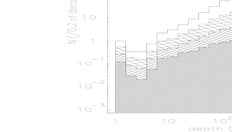
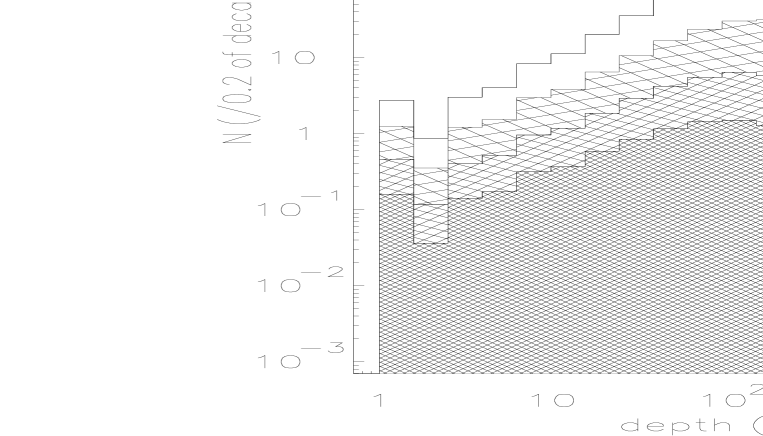
Figure 5: Histograms of muon origin levels for 10⁷ GeV protons (results of Monte-Carlo simulation) [17, Attallah, Szabelski et al., 1995]).

Figure 6: Histograms of muon origin levels for 10⁷ GeV iron nuclei (results of Monte-Carlo simulation) [17, Attallah, Szabelski et al., 1995]).

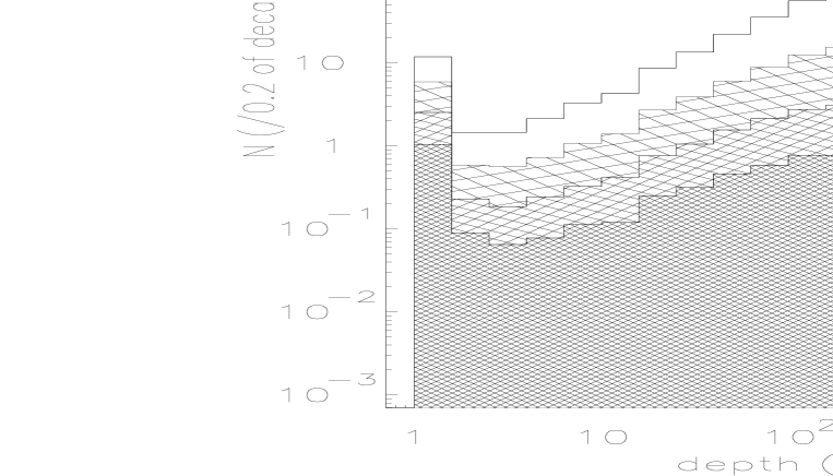
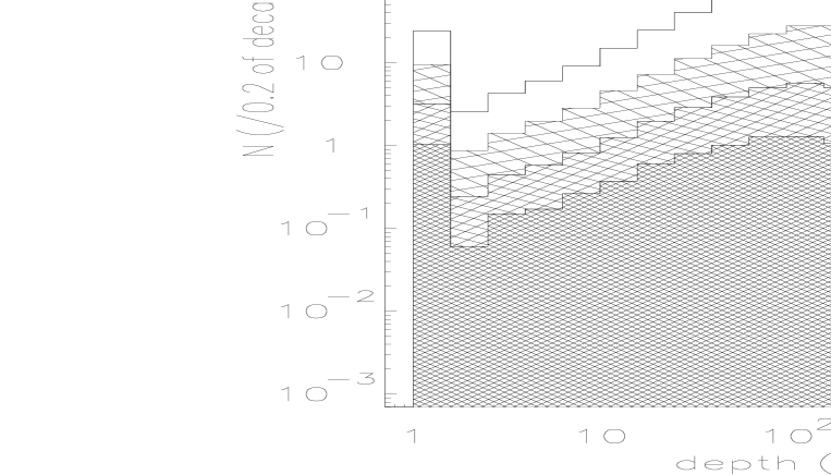
Figure 7: Histograms of muon origin levels relative to the first interaction for 10⁷ GeV protons (results of Monte-Carlo simulation [17, Attallah, Szabelski et al., 1995]).

Figure 8: Histograms of muon origin levels relative to the first interaction for 10⁷ GeV iron nuclei (results of Monte-Carlo simulation) [17, Attallah, Szabelski et al., 1995]).

3.2 High energy cosmic rays mass composition and underground measurements of muon groups.

Measurements of high energy CR muons can be used to study high energy nuclear interaction properties and mass composition of the primary cosmic rays. These muons are decay products of high energy pions and kaons of extensive air shower (EAS). Some pions and kaons can decay, other would interact. Therefore the number of muons depends on relation between probability of decay vs. probabilities of interaction or not–to–muon decay. It is clear that deeper in the atmosphere its density is larger and decays are relatively less probable than interactions as compared with the higher altitudes. On another side the number of energetic pions and kaons in the EAS has a maximum at the altitude which depends on the primary particle energy, mass, first few interactions heights and multiplicities of hadron production, etc. So the parent muon particles can originate at relatively high altitude i.e. near to the first interaction, and bring information about the EAS development in the upper layer of the atmosphere.

Figure 9: Average number of muons generated in EAS vs. energy of the primary particle as results of M-C calculations. Different curve modes relate to primary proton and iron nuclei. Results of superposition approach and fragmentation model are shown for comparison.
Four sets of different curves relate to four muon energy thresholds; from top to bottom: 200 GeV, 560 GeV, 1400 GeV and 3160 GeV. (Figure from [17, Attallah, Szabelski et al., 1995]).

Measurements of muon groups, i.e. simultaneous registration of number of parallel muons, play a special role. The experiments for muon group studies have areas from $\sim$10 m² to $\sim$300 m². They are placed relatively deep underground to limit the minimum energy of muons at the ground level to above $\sim$40 GeV (which is different for different experiments). The ground above the experiment absorbs the electromagnetic component (electron/positron and photons) of associated EAS as well as low energy muons. These are relatively low energy particles which originate much lower than most of high energy muons. Therefore underground measurements of high energy muons are in some sense equivalent to EAS observations at high altitude.

In the proton induced showers the average number of high energy muons depends on their energy, proton energy and the zenith angle. For CR proton energy (E_p) above approximately 20 times the muon threshold energy (E${}_{\mu\,\rm th}>{\rm 40~{}GeV}$) (to escape from the complicated near–to–threshold relation) the predicted total average number of muons with energy above E${}_{\mu\,\rm th}$ is proportional to E${}_{\rm p}^{0.7-0.8}$. The power index in this relation depends on the high energy interaction model used in the calculations. Higher multiplicity models predict higher power index.
Since high energy muons originate high in the atmosphere, calculations of predicted number of muons in EAS are sensitive to the interaction model used in Monte–Carlo program (see Figures 8 and 8, where one can notice that most of high energy muons orginate within 200 g/cm² from the first interaction). Results of measurements of single muon spectra in CR are related to properties of fragmentation region of high energy interaction models whereas muon group rates correspond to high multiplicity (central) region of high energy interation.
For CR nuclei (with atomic mass A) having the energy E_A = A$\cdot$E_n the total predicted average number of muons with energy above E${}_{\mu\,\rm th}$ is larger than for proton shower (E_p=E_A), provided that E_n is also well above E${}_{\mu\,\rm th}$. When the primary CR particle nucleon has energy not much higher than the required muon threshold energy then the corresponding relation between nucleon energy and the number or muons has not a power law form with the power index of 0.7–0.8. The relation in this threshold region is much steeper.
The simplest approach to evaluate the number of muons generated by the primary CR nucleus is the superposition model. In this approach it is assumed that the number of high energy muons (N${}_{\mu\,\rm A}$) generated in the shower originated by primary nucleus of energy E_A = A$\cdot$E_n is equal (on average) to the number of muons which would be produced in A showers originated by protons (or neutrons) with energy E_n: N${}_{\mu\,\rm A}($E_A) = N${}_{\mu\,\rm A}$(A$\cdot$E_n) = A$\cdot$N${}_{\mu\,n}$(E_n).
The more realistic model of primary CR nucleus interactions in the atmosphere assumes its destruction in a number of subsequent interactions. The destruction level depends on the interaction parameter. Such a model, presented in [42, Capdevielle, 1993] assumes the abrasion of incident and target nuclei (which is the interaction parameter dependent) as well as some evaporation of nucleons from excited fragments after the collision.
Calculations of predicted number of muons associated with primary CR nucleus were performed using both models for comparison. The important differences were noticed which in the first approximation show smaller high energy muon production for the abrasion and evaporation model as compared with the superposition model (see Figure 9). Some results of these calculations are presented in Section 3.3.4 on page 3.3.4.

3.3 Monte–Carlo simulations of high energy muon shower development in the atmosphere.

To interpret the experimental data on muon groups they were compared with the results of Monte–Carlo simulations of EAS development.

3.3.1 General information about the Monte–Carlo simulations of EAS development.

To compare results of models of high energy CR particle interactions the Monte–Carlo simulations of EAS development were performed. The first results were obtained at the University of Bordeaux using the large VM–System IBM computer, and then the code has been adapted to NDP Fortran with the UNIX–System on the PC computer in Łódź, and then to Digital FORTRAN on Alpha stations in Perpignan and in Łódź and finally to PCs using Fortran to C converters, ‘DJGPP’ compiler, and go32.exe program. During the Monte–Carlo simulations usage of most program arrays was monitored, to prevent over–writing.

In the presented analysis the EAS development has been simulated using the program code written by J. N. Capdevielle with some modifications related to the high energy muon group studies:

1. information about muons at the program output,

2. trace of hadrons with energy above 200 GeV, only (i.e. above the muon threshold).

The hadron interactions were treated according to dual parton model ([41, Capdevielle, 1989]) with some further modifications to adjust results to experimental data on particle production in high energy interaction. The air (the target) has been treated as containing atoms with A=14, only. The atmosphere pressure–height relation has a form:

$$\rm h(km)=\ln\left(\frac{\textstyle 1034}{\textstyle x}\right)\cdot(0.002375x+6.7625)\,\frac{\textstyle 1}{\textstyle\cos\it\theta}$$

where x is depth in the atmosphere in $g/cm^{2}$. This relation agrees with the US Standard Atmosphere (see preprint [40, Capdevielle et al., 1992]).

The nucleus–nucleus interactions were treated according to the abrasion–evaporation model ([42, Capdevielle, 1993]). Results were compared with the superposition approach to description of nucleus–nucleus interactions, and this problem will be discussed later.

3.3.2 Brief description of high energy muon group rate evaluation.

In the first step number of EAS were simulated and results were stored in memory. The procedure looks as follows:

1. The primary particle atomic numbers A were 1, 4, 14, 28 and 56,

2. the zenith angle $\theta$ was set to 10^∘,

3. the primary cosmic ray particle energy $E_{CR}$ varied from the threshold energy related to 200 GeV muon production in EAS to $10^{7.5}$ GeV/nucleus with the 0.1 step in logarithmic scale,

4. for each A and particle energy $E_{CR}$ the number of EAS simulations have been performed and information on first interaction and high energy muons was stored for further analysis. The number of simulated EAS varied from 1000 near the threshold CR particle energy to 100 at the highest energies. For each muon above the muon threshold energy (for this simulation: 200 GeV) its x, y position at the observation level, energy, parent particle type (i.e. pion or kaon) and the parent particle production height were stored.

Some simple properties like the average muon number, muon number distribution, correlation of muon number with the parameters of the first interaction, muon lateral distribution, etc. could be performed at this stage (see Figures 6, 6, 8 and 8).

While performing our calculations we have neglected some related problems. These seem to play less important role in the large muon group analysis. Incorporating them into the scheme of calculations would significantly enlarge the time of computing. Namely, we have neglected:

1. the influence of the Earth’s magnetic field on $\mu^{+}$, $\mu^{-}$ group:

   $$r_{G}/(1~{}m)=\frac{\textstyle p/(1~{}GeV/c)}{\textstyle 0.3\,\cdot\,B_{\textstyle\perp}/(1~{}T)},\rule{28.45274pt}{0.0pt}p\approx 200~{}GeV,\rule{28.45274pt}{0.0pt}B_{\perp}\approx 20\mu T\,=\,0.2~{}G$$

   $r_{G}$ = 3.3 10⁷ m is muon curvature radius. For muon production at altitude 15 km the displacement is $\approx$3.4 m due to magnetic field deflection. This can be compared with the displacement due to transverse momenta in pion or kaon production processes: $<p_{t}>\approx$ 0.4 GeV/c, gives 30 m for production at 15 km and 200 GeV/c muon, i.e. nearly 10 times more.

2. muon energy losses were treated as average for all muons (as an $E_{\mu\,\rm th}$ – muon energy threshold), whereas for large muon energies, energy losses are not uniform. However, since the analysis is related to large muon groups, this effect does not play an important role.

3. elastic scattering of muons in the rock was neglected i.e. their trajectories were straight lines.

4. we have performed simulations for one zenith angle $\theta$ of incident primary CR particle, and used these results for the whole nearby range of zenith angles (e.g. for $\theta<20^{\circ}$ we have used results obtained from calculations assuming $\theta=10^{\circ}$).

5. we assumed a circular shape of detector with the same effective area.

At the present stage of muon group events analysis the above listed approximations do not seem to produce effects which would change the interpretation of data.

3.3.3 Total number of high energy muons produced in EAS.

The total number of muons with energy above a threshold (although not measured in most experiments) is a convenient value to compare between different calculations. Performing a number of M–C simulations of EAS for a fixed primary CR particle type and energy, the average number of muons can be found together with its distribution. The average number of muons depends on primary CR particle energy. It grows fast with particle energy near the muon production threshold energy and then grows according to the power law.

Figure 10: Results of Monte-Carlo simulation of average number of high energy muons in EAS generated by protons and iron nuclei and approximate fit [16, Attallah, Szabelski et al., 1995] [17, Attallah, Szabelski et al., 1995].

Table 3: Parameters for equation 1.

	A	$\gamma$	$C$	$\alpha$	$B$	$\beta$
protons	1	1.58	6.0	0.78	0.6	13.0
iron	56	1.68	6.0	0.81	0.65	10.0

In the Figure 10 the average number of muons above four threshold energies is illustrated for primary protons and iron nuclei. Lines represent the parametrization:

$$<{\rm N}_{\mu\,\rm A}>={\rm A}\cdot C\cdot~{}\frac{\textstyle E_{\rm n}^{\alpha}}{\textstyle E_{\mu\,\rm th}^{\gamma}}\,\cdot~{}\,\left(1.0-B\cdot\frac{\textstyle E_{\mu\,\rm th}}{\textstyle E_{\rm n}}\right)^{\beta}$$ (1)

where $E_{\rm n}$ = $E_{\rm CR}$/A, $E_{\mu\,\rm th}$ is the muon energy threshold and other parameters are in the Table 3.
For muon energy threshold $E_{\mu\,\rm th}$ = 200 GeV the distribution of N_μ is Gaussian around $<{\rm N}_{\mu}>$. For M–C simulations of 1000 EAS for each CR primary energy in the range (10⁵–10^7.5 GeV) the number of events with N_μ can be parametrized as follows:

$${\rm N}_{1000}({\rm C},{\rm N}_{\mu},<{\rm N}_{\mu}>,\sigma)={\rm C}\cdot\frac{1}{\sigma\sqrt{2\pi}}\cdot\exp\left[\frac{\textstyle-({\rm N}_{\mu}-<{\rm N}_{\mu}>)^{2}}{\textstyle 2\sigma^{2}}\right]$$ (2)

$$\begin{array}[]{lrcccccl}\rm where~{}for~{}protons:&{\rm C}&=&995&-&11.2&\cdot&{\rm log}_{10}(\rm E_{\rm p}~{}/{\rm 1~{}GeV})\\ &{\rm log}_{10}(\sigma)&=&-2.9&+&0.707&\cdot&{\rm log}_{10}(\rm E_{\rm p}~{}/{\rm 1~{}GeV})\\ \rm and~{}for~{}iron:&{\rm C}&=&1022&-&11.3&\cdot&{\rm log}_{10}(\rm E_{\rm Fe}/{\rm 1~{}GeV})\\ &{\rm log}_{10}(\sigma)&=&-2.8&+&0.683&\cdot&{\rm log}_{10}(\rm E_{\rm Fe}/{\rm 1~{}GeV})\\ \end{array}$$

and $<{\rm N}_{\mu}>$ is given by the formula 1 for E${}_{\mu\,\rm th}$ = 200 GeV.

The slope of $<{\rm N}_{\mu}>$  vs. $E_{\rm p}$ dependence (at the power law part) is usually related to the properties of the first interaction of CR particle, and particularly to the multiplicity of secondary particles produced then. For some calculations made in the past assuming the Feynman scaling ([58, Feynman, 1969]) the slope has a value of $\approx$0.7, and for extremely large scaling breaking of [97, Wdowczyk, Wolfendale, 1979] model its value was equal to $\approx$0.85. The difference 0.15 in the power law dependence gives a factor of 1.4 in the difference in $<{\rm N}_{\mu}>$ over the energy range of one order of magnitude and a factor of 2 over two orders of magnitude in the $E_{\rm p}$ energy range. The $<{\rm N}_{\mu}>({\rm E}_{\mu}\geq{\rm E}_{\mu\,\rm th})$ vs. E_p relation can be normalized (and verified) in the near–to–threshold proton energy range by evaluation of predicted single muon flux:

$$I_{\mu~{}m=1}({\rm E}_{\mu}\geq{\rm E}_{\mu\,\rm th})=\int~{}\,j_{\rm p}({\rm E}_{\rm p})~{}\cdot<{\rm N}_{\mu}>({\rm E}_{\rm p})~{}\,~{}d{\rm E}_{\rm p},$$

where $j_{\rm p}$(E${}_{\rm p})$ is a differential CR proton energy spectrum. The experimentally measured muon intensity for E${}_{\mu}\geq$ 200 GeV is about 3.2 $\cdot$ 10^-2 muons per (m² sec sr), and one gets the same value using CR energy spectrum and composition presented in the Appendix B on page 7 with about 30% contribution from components heavier than protons in CR flux. Using JACEE CR energy spectrum [14, Asakimori et al., 1995] one gets 2.5 $\cdot$ 10^-2 muons per (m² sec sr) with about 40% contribution from heavier components. The single muon flux is relatively well measured (for E${}_{\mu\,\rm th}>$200 GeV this means the accuracy within a factor of 1.5, mostly due to the difference in muon energy estimation in different experiments; the project “L3+Cosmics” gives opportunity to measure single muon flux with accuracy better than 1% for E${}_{\mu}<\sim$1000 GeV, using “L3” detector at LEP in CERN). In these calculations the spectral index in the power law relation of $<{\rm N}_{\mu}>$  vs. E_p is equal to $\approx$0.8. This value is somewhat above presently accepted value 0.76 which comes from simple consideration and relates to the experimentally measured power index in the muon group multiplicity distribution, where in a large detector rate of the large muon group with m muons is proportional to m^-3.3.

Some assumptions made in presented simplified estimation of power index are not sufficiently exact. Since the CR energy spectrum has a power law energy dependence with the index of $\approx$–2.7 (below 10⁶ GeV, at least) the average effective energy required to produce N${}_{\mu}^{0}$ in the shower is somewhat lower than the energy required to produce $<{\rm N}_{\mu}>={\rm N}_{\mu}^{0}$. The ratio between these energies is not a constant factor since the N_μ distribution around $<{\rm N}_{\mu}>$ for the constant CR particle energy is wider for smaller energy than for higher energy (where it seems to be of Gaussian shape with the width of 0.15 in $\log({\rm N}_{\mu})$ scale, and not $<{\rm N}_{\mu}>$, nor E_CR dependent at higher energies). The above effect of changed width in N_μ distribution for constant E_CR requires a bit faster growing of $<{\rm N}_{\mu}>$  vs. E_CR than predicted by the formula 1 to get agreement with observed muon group multiplicity rate. It is necessary to mention that the power law index of CR particles energy spectra is not known absolutely well, and different measurements gave very inconsistent results ([13, Asakimori et al., 1993]).

Figure 11: N_μ distributions (E${}_{\mu}>$ 200 GeV) as result of M–C simulations for iron nuclei primary CR particle. Solid lines are results from fragmentation model for 1000 EAS – see formulae 2 and 1 for iron – for three primary energies E_Fe = 10^6.5, 10⁷ and 10^7.5. Dashed-dotted line represent predictions from the superposition approach – rescaled from formulae 1 and 2 for protons at 56 times smaller energy.

3.3.4 High energy muon multiplicity predicted in superposition model and
abrasion/evaporation model of nucleus–nucleus collision.

Some comparison between two high energy models of nucleus–nucleus interaction is presented (see Figure 11).

1. The first model is the superposition model which is widely used in EAS physics. The result of interaction of a cosmic ray nucleus with nuclei of the atmosphere is replaced by superposition of each nucleon interaction with the atmosphere. If CR nucleus has the energy E_A and the atomic number A then predicted results of the EAS development is obtained as a random superposition of A showers initiated by protons with the energy E_A/A, i.e. nucleon energy. The results of nucleus interaction were replaced by the sum of A proton induced showers randomly sampled from the large storage or subsequently generated.

2. The abrasion/evaporation model of nucleus–nucleus collision describes CR nucleus interaction in the atmosphere as subsequent fragmentation of incident particle together with evaporation of some nucleons from the excited fragment as presented in [42, Capdevielle, 1993] and [18, Attallah, Szabelski et al., 1996].

In both cases nucleon and other hadron interactions with air–nuclei were described using developed version of “dual parton model” presented in [41, Capdevielle, 1989]. Details copncerning the atmosphere, particle decay parameters, cross sections parametrizations, multiplicities of secondary particles etc. were summarized in [40, Capdevielle et al., 1992].

3.4 Experimental observation of muon groups.

3.4.1 Muon and neutrino telescope of the Baksan Neutrino Laboratory of the Russian Academy of Sciences.

The Baksan Neutrino Observatory is placed in northern Caucassus in the valey of Baksan river, about 30 km from Mt. Elbrus. The geographical coordinates are N 43.42^∘, E 42.67^∘. The muon telescope is placed inside the mountain in a large cavity, which is made in the horizontal tunnel, 500 m from the entrance. The mountain slope is $\sim$30^∘, so above the telescope there is $\sim$300 m of rock, i.e. $\sim$850 hg/cm² (rock’s density is 2.70$\pm$0.03 g/cm³, Z/A=0.495, Z²/A=5.88, [65, Gurencov, 1984]). The rock above the telescope absorbs most of cosmic ray secondary particles; only neutrinos and high energy muons can penetrate to the detector. The muon threshold energy above the rock to penetrate it is $\sim$250 GeV for vertical direction, and $\sim$190 GeV for the direction of smallest rock’s depth ($\theta~{}\approx$ 30^∘ inclined to the entrance). Muons coming from directions of large depths are also observed, even from direction pointing below the horizon. The latter are interpreted as being produced in energetic neutrino interactions in telescope vicinity.

The Baksan muon and neutrino telescope has a size of 16.7 m$\times$16.7 m$\times$11.1 m. It consists basically of 3150 liquid scintillation counters, each of size 0.7 m$\times$0.7 m$\times$0.3 m. Scintillation counters make 4 horizontal layers (floors) separated by $\sim$3 m and 4 vertical side walls. Every scintillation counter is seen by a single FEU–49 photomultiplier. Two–fold information is collected: an impulse signal from the anode and an amplitude signal from the 5^th dynode. The signal from the anode gives the information that the energy released in the scintillation counter exeeded 12.5 MeV threshold (corresponding to 1/4 of energy released by relativistic, single charged vertical particle). The amplitude signal is used to determine energy released in the scintillation counter when this energy is in the range 0.5 GeV – 500 GeV.

$${\rm E}\,=\,0.5\,{\rm GeV}\,\cdot\,1.23^{\rm\,n-1},$$

where E is energy released and n is a channel number. The relative time of first impulse in each plane is registered and these times can be used to determine the direction (e.g. up or down) of the event. The absolute time of the event is also recorded.

The telescope has many tasks:

• measurements of single muon flux from different directions,

  • studies of muon attenuation in the rock,

  • studies of cosmic ray anisotropy and time variation,

  • search for cosmic ray point sources,

  • studies of dependence of muon flux on atmospheric pressure and temperature of the atmospheric upper layers,

• neutrino astrophysics,

  • search for signals from collapsing stars (the explosion of the Large Magellanic Cloud supernova in 1987 has been probably observed),

  • search for neutrino sources,

• search for proton decay,

• studies of high energy muon interactions,

• studies of muon groups.

The number of tasks requires large amount of information to be registered.

3.4.2 Data selection and muon group analysis.

The muon groups are studied for information about high energy cosmic rays mass composition and about properties of high energy nuclear interactions. These studies require an extraction of rare muon group data from the bulk of all registered information stored on magnetic tapes. Muon group data are then stored in disk memories for further analysis. The data selection is not an easy task. Small muon groups get some “muon group flags” already in the “on line” analysis. Large muon groups data might be classified incorrectly, or they might be too complicated for the “on line” program and they might have no classification in that case.

Originally we had used following criteria for large muon group selection:

1. minimum 30 hit scintillation counters in each horizontal layer (floor) of the telescope,

2. the number of hit scintillation counters in each horizontal layer should differ from the average number of hit counters in horizontal layers for less than
   3 $\cdot~{}\sigma$ = 3 $\cdot~{}\sqrt{\rm average~{}number}$.

The first criterion selects large events, and the second was applied to eliminate large electromagnetic or hadronic cascades originated in high energy muon interaction in the telescope vicinity.
After a couple of years we have learnt that electromagnetic cascades are more common in large muon groups than we had estimated originally. The second criterion has eliminated some part of muon groups (with $\sim$100 muons inside the telescope) in which electromagnetic cascades where also present. For the very large muon groups with more than 1/3 (above 1200) hit scintillation counters the second criterion was fulfilled despite the presence of large electromagnetic cascades.

At present we use still another criterion: minimum number of hit scintillation counters in the whole telescope. For basic selection we use 100 as a minimum number, but we also use 300 and 600 for selection of very large muon group events. The basic criterion (100) is very often fulfilled by small muon groups (few muons) with electromagnetic cascades (few muon tracks are seen then). Of course most small muon group registrations do not fulfil the basic criterion, since they do not have electromagnetic cascades.
For muon groups with $\approx$25 muons inside the telescope the basic criterion is of “minimum bias” type, since the average muon hits about 4 scintillation counters while passing through the telescope.

3.4.3 Muon multiplicity distribution in Baksan telescope.

All muons in the group are parallel. The incoming direction of muon group can be found by searching for co–linear pattern of hit counters from different layers. The difference between time registration of the first hit counter in each plane can be used as a very crude information (for events with a large number of hit scintillation counters in a plane, the measurement of time of the first hit counter is uncertain for hardware reasons). Co–linearity is investigated by the computer program for automatic data analysis. The program finds incoming directions for most events but large groups. Directions are verified “by eye” using the program for visualisation of events. Corrected direction (when they are determined) are stored in a data base along with the automatic estimation.
We have selected events with the zenith angle $\theta~{}<$ 20^∘ for the purpose of our studies, because it is easier to compare experimental results with predictions when there are events with similar threshold and the same zenith angle range. Let us notice that the rate of muon group events is related to the depth of rock, and the maximum rate is from direction to the entrance to the tunnel and $\theta~{}\approx$ 30^∘ (i.e. outside our $\theta$ range).

In most of registered muon group events it was possible to determine the gradient of muon tracks density in the plane perpendicular to event direction. The muon group core is near to extrapolated track of primary cosmic ray particle which has generated extensive air shower. The average distance of a muon from the muon group core is about 25 m for muons with energy above $\sim$250 GeV. Large size of the telescope allows to measure the lateral distribution of high energy muons in the shower. In about a half of registered muon group events the muon group core is inside the telescope. Near the core the average muon energy is higher than far from the core because more energetic muons have narrower lateral distribution (for similar average lateral momentum they have larger longitudinal momentum). In this region the probability of muon interaction and creation of electromagnetic cascade is larger since muon interaction cross section depends on energy.

Figure 12: The figure presents correction factor from “observed” number of muons to real muon number which has been used in our muon group data analysis. The top line (dashed) was obtained by simulations when the EAS axis was inside the telescope, the bottom one (dashed–dotted): axis outside, and the central (solid) is the average taking into account acceptance; the central was used to produce the Figure 13.

Another very important problem is the spatial resolution of the telescope. It is limited to the single scintillation detector size: 0.7 m$\times$0.7 m$\times$0.3 m. Very large muon showers could have muon densities high enough to allow two or more muons to pass through the same detectors. They would be interpreted as a single muon since the amplitude measurement starts at energy released above 500 MeV (i.e. above about 10 relativistic particles).
This problem and ‘an opposite problem’ of electromagnetic and hadronic cascades induced by muons in the detector was solved in detector simulations. We made a computer program to count the trajectories of muons taking into account the geometry of the telescope (the detectors layout). Then another program simulated the muon shower in the telescope taking into account muon lateral and energy distributions and detector construction (i.e. muon interactions with telescope) for different muon groups with shower core inside and outside the telescope. This program gives results in the same format as real data output, so the program counting the tracks could be used. As a result we have worked out the correction factors (shown in the Figure 12) to transform the number of tracks identified by the program to number of muons in the telescope.
Running the track counting program on the real data we have obtained results shown in the table 4 [96, Voevodsky, Szabelski et al., 1994].

Table 4: Counts of muon tracks (n) in Baksan telescope. Results were grouped in number of track ranges. The number of events (N) with the muon tracks (n) within the n range corresponds to indicated time exposure. To produce muon multiplicity distribution shown in the Figure 13, the number of tracks (n) was corrected (see text).

n range	21–30	31–40	41–50	51–70	71–100	101–130	130–170	$>$ 170
$<$n$>$	24.5	34.6	45.0	58.6	80.1	114.2	143.8
N	80	277	106	98	39	32	13	4
time (sec)	1.7 106	1.9 107	1.9 107	1.9 107	1.9 107	4.2 107	4.2 107	4.2 107

The number of tracks (n) obtained as a result of track counting program needs to be related to the number of muons (m) in the telescope. We have used the average conversion factor presented in the Figure 12. This takes into account the probability of a few muons going close together and mimiking one, cascades triggered by a muon in the telescope, and various positions of the EAS core relative to the detector area.
Results are presented as a open circles in the Figure 13 (errors are statistical). Black points represent low muon multiplicity group rates, which were obtained from smaller exposure. For low multiplicity groups no correction was applied because the muon density was small enough. This figure is an integral muon multiplicity distribution for muons with E${}_{\mu\,\rm th}>$ 250 GeV, only muons within the telescope, group directions with zenith angle less than 20 degrees. Different time exposures used for determining number of events with different multiplicity were taken into account. The muon rate for the number of muons equal or greater than m was multiplied by m^2.3 for presentation. The distribution was normalized to the total number of muons registered in the telescope (the method presented in [47, Chudakov, 1979]).

Figure 13: The figure presents integral muon multiplicity distribution (E${}_{\mu\,\rm th}$ = 250 GeV) normalized to the total number of muons. The corresponding rates were multiplied by muon number in power 2.3. Black points were low multiplicity ones (no corrections), the open circles show high multiplicity muon rates [96, Voevodsky, Szabelski et al., 1994]. The curves correspond to calculated predictions using different primary energy spectra and mass compositions: dashed line – no “knee”, solid line – “knee” at 1.5 10¹⁵ eV/nucleon, dashed–dotted line – “knee” at 1.5 10¹⁵ eV/nucleus (see text for detailes).

The lines describe predictions obtained from calculations. Muon production for a given primary particle type and energy (i.e. EAS development, interaction parameters) were the same in all presented cases. The detailed calculations of high energy muon production using different interaction models show that the difference between models is smaller than the difference which is due to primary particle mass (atomic number). Therefore it is reasonable to examine first the prediction for various CR primary particles. The lines differ in the assumed cosmic ray mass composition and energy spectra. The highest, dashed line represents the case where the integral CR energy spectra have constant power index (= –1.7) for all types of particles and in all related energy range (no “knee”). The relative mass composition is the same as in low energy part of the next CR spectrum model. This is probably not a realistic case, since all EAS experiments show the “knee” (change of power index of distribution) in shower size distribution (estimated total number of electrons in EAS at observation level). It can be noticed that it does not describe the muon group data above m = 100.
The next is a solid line which represents the integral CR energy spectra which have a change of power index (the “knee”) from –1.7 below 1.5 10¹⁵ eV/nucleon to –2.1 above this energy. The relative mass composition (in energy per nucleon) is constant. The “knee” energy is given per nucleon, so the mass composition as seen in energy per particle is heavier above the “knee” than before, since the spectra of lighter components have the change of power indexes for smaller energy per nucleon, than the spectra of heavier particles. This line lies generally below the experimental points.
The bottom, dashed–dotted line corresponds to integral CR energy spectra which have the change of power index (the “knee”) at the same energy per particle for all nuclei present in CR at these energies: from –1.7 below 1.5 10¹⁵ eV/nucleus to –2.1 above that energy. This spectrum has a constant relative mass composition in energy per particle (i.e. per nucleus). The predictions are not consistent with muon group results presented in the Figure 13.
The spectra and mass compositions of cosmic rays are presented in the Appendix B on the page 7.
It is interesting to compare the Figure 13 (muon multiplicity rates in Baksan telescope) with Figure 9 (average number of muons produced in EAS). It gives an opportunity to estimate the primary CR particle energy related to observed muon multiplicity. Multiplicities 1 and 2 are mostly due to CR protons with energies 600 GeV – 3000 GeV (6 $\cdot$ 10¹¹ – 3 $\cdot$ 10¹² eV). The energies are lower than corresponding values for $<$N${}_{\mu}>$ shown in the Figure 9, since the proton spectrum is very steep. When higher muon multiplicities are observed, the total number of muons above the threshold energy in EAS is about 4 – 5 times larger than the number of muons in the telescope, because of the lateral spread. Observed multiplicities around 10 correspond to primary energy about 1.5 $\cdot$ 10¹⁴ – 4 $\cdot$ 10¹⁴ eV. Observed multiplicities around 100 require CR energies 3 $\cdot$ 10¹⁶ – 10¹⁷ eV. The largest events with multiplicities above 300 came from CR particles with energy above $\sim$1.5 $\cdot$ 10¹⁷ eV. Therefore a single detector can register events triggered by CR with primary energy from $\sim$600 GeV to more than 10¹⁷ eV, i.e. from relatively known energy region (interaction properties, mass composition) to energies 10⁵ times higher.
Results from two other large underground experiments have been published recently.

• The Soudan 2 detector ([72, Kasahara et al., 1997]) is at the depth of 710 m (muon energy threshold $\sim$ 700 GeV) and has dimensions 8 m $\times$ 14 m and 5.4 m in height. The results of muon groups measurements (multiplicity range from 1 to 12 in the detector) correspond to primary particle energy range 10¹² – 1.3 $\cdot$ 10¹⁶ eV.

• The MACRO detector has six ‘supermodules’, each is 12 m $\times$ 12 m $\times$ 9 m in size [10, Ambrosio et al. 1996]. The muon energy threshold is $\sim$ 1400 GeV. The results of muon groups measurements (multiplicity range from 1 to 39 in the detector) correspond to primary particle energy range 3 $\cdot$ 10¹² – 10¹⁷ eV [11, Ambrosio et al. 1996].

3.5 Future prospects of cosmic ray mass composition measurements.

The measurement of mass composition of cosmic ray energy spectra in energy range 10¹⁴ – 10¹⁶ eV is a target of a few large currently working or being constructed extensive air shower (EAS) experiments. They combine measurements of a few components of EAS for each event to more efficiently measure the primary CR particle energy and distinguish between different primary particle masses. Only in Europe we have:

• Experiment HEGRA placed at mountain altitude on Canary Islands, which registers electro–magnetic (E–M) component of EAS, low energy muons and Cherenkov radiation. It has been working already for a few years already.

• The KASCADE experiment placed near the sea level, beginning to register E–M particles, low energy muons and hadrons (large hadron calorimeter).

• The EAS–Top array, measuring at mountain altitude E–M component, low energy muons, Cherenkov light in coincidence with high energy muon (E${}_{\mu\,\rm th)}>$ 1400 GeV) large detector MACRO.

• The Andyrchi array, measuring E–M particles in coincidence with high energy muons (E${}_{\mu\,\rm th)}>$ 250 GeV) registered in the Baksan telescope (mountain altitude) ([6, Alexeev et al., 1993], [7, Alexeev et al., 1994]).

The general idea in most of these experiments is to measure components related to EAS energy (e.g. Cherenkov light, low energy muons or E–M particles) and relate them to components finally determined by the early stage of EAS development (i.e. high energy muons or Cherenkov light) which almost do not interact later, and therefore provide information closely related to primary particle.

The combination of Andyrchi EAS array with large underground muon telescope at Baksan looks very promising for CR mass composition measurements. The EAS array detectors lie on the area of 5 $\cdot$ 10⁴ m², it is on average 350 m above the muon telescope and the array covers 0.35 sr as seen from the telescope. This provides about one event per 10 sec in coincidence with the muon inside the underground telescope. This rate is more than 100 times higher than in the case of EAS–Top/MACRO experiments, since EAS–Top array is much higher above the muon detector (smaller solid angle) and the muon threshold is about 5 times bigger.
The results from Andyrchi/muon telescope EAS measurements should allow to narrow energy ranges discussed at the end of last section. This should provide some information about the CR mass composition in important high energy range.

The interpretation of EAS data becomes much reliable recently due to fast development of computing power. It is very important that computers are fast, have large memories and large disk space, which allow to run the EAS shower programs tracing millions of particles through the atmosphere. Even more important is the existence of reliable, publicly available and “friendly” large simulation programs for EAS studies. The most famous in our area is the CORSIKA code [40, Capdevielle et al., 1992] developed in Forschungszentrum Karlsruhe. It enables theoretical studies of different components of EAS. The comparison of its results with experimental data provides certain confidence about the model of hadronic interactions used in the program, as well as the overall modeling of tens of physical processes, which EAS particles undergo.

4 The highest energy cosmic rays

The highest energy cosmic ray (CR) events exceed 10²⁰ eV per particle. In this section some results of studies of CR with energy above 10¹⁹ eV are presented.
The main reasons for studying the highest energy cosmic rays are:

• nuclear interaction properties,

• limits on cosmic ray energy,

• acceleration mechanism,

• source problem.

However, it should be clear that the present stage of research in this direction might be called: the beginning. There are no scientifically justified answers to above listed interesting problems.

4.1 Detectors of the highest energy cosmic rays

CR particles with energy above 10¹⁹ eV are very rare – about 1 event per 1–2 years on 1 km² sr [50, Cunningham et al., 1980]. Each event produces huge cascade of secondary particles in the atmosphere. For these two reasons the arrays for observing such events should have large area (to increase the number of observed events), but they do not need to have detectors very close to each other (since the size of extensive air shower region with detectable particle density is large). The observations last long and detectors undergo modernizations and changes during the operation. Usually the array sensitivity depends on EAS energy, zenith angle, position. For running experiments the exposure grows in time. Therefore given below sizes or exposures are approximate and valid for the time of reference.
The largest arrays for detecting CR of the highest energies are:

• Haverah Park (England, $\sim$12 km² [34, Bower et al., 1983]) – 45 km² yr [22, Bell et al., 1974],

• SUGAR - Sydney (Australia, $\sim$110 km² [100, Winn et al., 1986]) – 175 km² yr [22, Bell et al., 1974],

• Volcano Ranch (USA), – 30 km² yr [22, Bell et al., 1974],

• Yakutsk (Syberia) – 33 km² yr [22, Bell et al., 1974], – 170 km² yr sr [34, Bower et al., 1983],

• Akeno Giant Air Shower Array (AGASA) (Japan – $\sim$100 km²) [46, Chiba et al., 1991],

• Fly’s Eye (Utah, USA, another method of detecting high energy CR via detection of light from fluorescence of atmospheric molecular nitrogen due to ionization and excitation caused by relativistic particles of the extensive air shower ([21, Baltrusaitis et al., 1985] and [75, Linsley, 1978]), Fly’s Eye acceptance varies from $\sim$1 km² sr at 10¹⁷ eV to $\sim$1000 km² sr at 10²⁰ eV, although the observation time efficiency is $\sim$6% [44, Cassiday, 1985], (the highest energy observed event of 3$\cdot$10²⁰ eV was reported recently, [28, Bird et al., 1993]).

Only Akeno, Yakutsk and Fly’s Eye detectors are working now.

4.2 Data availability

The data on the highest energy events and descriptions of detectors from Volcano Ranch, Haverah Park, SUGAR and Yakutsk were printed [76, Linsley, 1980], [49, Cunningham et al., 1980], [101, Winn et al., 1986] and [56, Efimov et al., 1988]. The estimated energy, zenith and azimuth angles, direction in equatorial coordinate system, time of the event and position of the shower core are available. For some events the responses of all detectors of the array are also given. Figure 14 shows directions of showers with energy above 3$\cdot$10¹⁹ eV.

Figure 14: Hammer–Aitoff plot (celestial coordinates) with highest energy data compilation (E${}_{CR}>$ 3$\cdot$10¹⁹ eV).

4.3 Astrophysical information

The classical discussion of astrophysical problems related to the highest energy CR can be found in [69, Hillas, 1984].
The energy spectrum as measured by Haverah Park, Volcano Ranch (the Northern hemisphere) and SUGAR (the Southern hemisphere) is discussed. It has a power law energy dependence below 10¹⁹ eV (with a power index $\sim$–3 for the differential energy spectrum) and shows some flattening for the higher energies. Despite the difficulty of energy estimation and different methods used in different experiments for this purpose the energy spectra show similar energy dependence. However, to get the same intensities for these 3 experiments it was necessary to renormalize the SUGAR events energy by 15% (which is within the possible systematic error since SUGAR detected only low energy muon component of EAS) [90, Szabelski et al., 1986]. The intensity difference could be more important as it might reflect the difference between the Northern and Southern hemispheres, which could relate to mass composition of highest energy CR and the galactic magnetic fields configuration in the Solar System vicinity (M. Giller, private communication, 1993). Mass composition of CR at these energies is not known experimentally, of course.

The incoming direction of very high energy CR is measured quite well. This information and time of the event are much more reliable than any other measured value (e.g. energy) for this energy CR. No important time variation nor correlation were found during the data analysis. Also the directional distribution seems to be very uniform. These observed features are very difficult to interpret “constructively” for studies of origin and source problem of CR in this energy range.
Charged particles have bent paths due to galactic magnetic fields. The CR particle Larmor radius r_L = 1.08 E₁₅/(Z B_μG) pc, where E₁₅ is equal to particle energy in 10¹⁵ eV unit, Ze is its charge, B_μG is the magnetic field normal to the particle momentum in $\mu$G and 1 pc $\approx$ 3.08$\cdot$10¹⁸ cm. For typical average values of B${}_{\mu\rm G}\approx$ 3 and particle energy of 10¹⁹ eV, r_L $\approx$ 3 kpc for protons, and r_L $\approx$ 50 pc for iron nuclei. The “local” thickness of the galactic disc defined as a length of column containing half of neutral hydrogen is equal to $\sim$100 pc. For these reasons one might expect to observe anisotropy of arrival direction of the highest energy CR if their sources were galactic or relatively local.

4.3.1 n–point correlation function

Since there are no obvious directions on the sky which the highest energy CR events would ‘prefer’, it is good to have a well defined method of searching for possible local anisotropies in experimental data. This method should meet following requirements:

• work for small and large statistics,

• allow for different angular size of clustering,

• allow for statistical comparison between observations and predictions.

The last point is particularly complicated because experiments are located at different positions on the earth, they have different acceptance (which is also zenith angle dependent). So the expected sky coverage is not uniform. We found that the n–point correlation function meets above requirements.

Figure 15: The declination distribution of arrival direction of CR from the zenith angle distribution (lines) and those observed (histograms). The compilation of data from experiments at Sydney, Haverah Park, Volcano Ranch, and Yakutsk. Upper histogram and line represent CR events with energy E${}_{CR}>$ 10¹⁹ eV whereas lower histogram and line correspond to E${}_{CR}>$ 3$\cdot$10¹⁹ eV.

We define the n–point correlation function for a sample containing M events as follows [45, Chi, Szabelski et al., 1991]:

$${\rm w}_{n}(\theta)~{}=~{}\sum_{\textstyle i=1}^{\textstyle M}\,\vartheta\left(\sum_{\textstyle j=1,j\neq i}^{\textstyle M}R(\theta_{ij})~{}-~{}n\right)$$

where     $\vartheta(x)=\left\{\begin{array}[]{rrc}1&{\rm if}&x\geq 0\\ 0&{\rm if}&x<0\end{array}\right.$       and     $R(\theta_{ij})=\left\{\begin{array}[]{rrc}1&{\rm if}&\theta_{ij}\leq\theta\\ 0&{\rm if}&\theta_{ij}>\theta\end{array}\right.$

$\theta_{ij}$ is the angular separation of two events on the sky.
It is possible to calculate the predicted values of w${}_{n}(\theta)$ for each declination (declination band). Let $\varrho$ be the density of events in a declination range (i.e. number of events per steradian) and let there be M events in this range. Then, in an area limited by the circle of radius angle $\theta$, equal to S = 2 $\pi$ (1–$\cos\theta$), the average number of particles m = S $\varrho$ is expected. The predicted value of w${}_{n}(\theta)$ can be taken from the Poisson distribution:

$${\rm w}_{n}(\theta)=M\cdot\sum_{\textstyle i=n}^{\textstyle\infty}\left(\exp(-m)\frac{\textstyle m^{i}}{\textstyle i\,!}\right).$$

The evaluation of the predicted values of w${}_{n}(\theta)$ was performed for declination bands (but not for right ascension nor galactic latitude bands etc.), because the exposure coverage is approximately the same along the whole band due to the daily rotation of the Earth. Then it is possible to search for any enhancement within one declination band (e.g. crossing with galactic plane) or even for larger structures appropriately evaluating predicted average number m.

4.3.2 Search for enhancements of ultra high energy cosmic ray arrival directions

In the paper [45, Chi, Szabelski et al., 1991] arrival directions of ultra high energy (UHE) CR were examined and here these results are presented. The CR events with energy above 10¹⁹ eV were used for the analysis. For these energies the Larmor radius is larger then 3 kpc for protons and 50 pc for iron nuclei (see page 4.3). Therefore one might expect some directional enhancement in the case of galactic orgin of these CRs. The bulk of observed events do not show any anisotropy, so the galactic disc is not a favourite place of UHE CR sources. We had searched for some grouping of UHE CR events, since it might indicate the direction of a (weak) source within several hundreds of parsecs from the Sun.

About 700 events from Volcano Ranch [76, Linsley, 1980], Haverah Park [49, Cunningham et al., 1980], SUGAR [101, Winn et al., 1986] and Yakutsk [56, Efimov et al., 1988] were summed up for the direction analysis of CR with energy above 10¹⁹ eV. Special attention was paid to the analysis method to be independent of any astrophysical model of UHE CR origin or propagation, i.e. instead of verifying some ideas we used the correlation analysis presented in the section 4.3.1.
First the directions of UHE CR were grouped according to their zenith angles and according to their declination angles. Assuming the azimuth angle symmetry and the equal coverage of the sidereal day by the working time and taking the actual zenith angle distribution it was possible to evaluate the predicted declination distribution for each experiment separately. The sum of declination distribution from all four experiments together with predictions is shown in the Figure 15.

The predicted and actual distributions agree well. They were used to evaluate the average “predicted” density of UHE CR events in declination bands for the n–point correlation function analysis.

Figure 16: Hammer–Aitoff plot (celestial coordinates) of “groups” of more than 5 CR events (E$>$10¹⁹ eV) within 6^∘ of an event with E$>$3$\cdot$10¹⁹ eV (plotted as squares) and groups of more than 3 CR events within (E$>$3$\cdot$10¹⁹ eV) within 6^∘ listed in the table 5 (plotted as circles) (those statistically significant are listed in the table 5 and discussed in the text). The galactic plane and galactic poles are indicated.

The n–point correlation function analysis (see section 4.3.1) was performed for n up to 5 and $\theta$ up to 40^∘. Different event energy requirements were examined:

1. all events with energy above 10¹⁹ eV,

2. all events with energy above 3$\cdot$10¹⁹ eV and

3. the central particle with energy above 3$\cdot$10¹⁹ eV but other with energy above 10¹⁹ eV.

We have found a general agreement between observed and predicted values of w${}_{n}(\theta)$ in different declination regions and energy bands, with two exceptions, both when all events have energy above 3$\cdot$10¹⁹ eV (see the table 5 for more details):

• for $-$90${}^{\circ}<\delta<-$60^∘ there is 1 event with 4 other events within 6^∘ of it, whereas 0.01 is expected (14 events in the region and a chance probability 6.6$\cdot$10^-4),

• for $-$60${}^{\circ}<\delta<-$30^∘ there are 3 events with 3 other events associated within 6^∘ whereas 0.067 is expected. There are also 3 other events in this region with 2 events associated within 6^∘, whereas 0.57 is expected.

Table 5: Positions of the central event of the UHE CR groups on the sky. All events in listed groups have E${}_{CR}>$ 3$\cdot$10¹⁹ eV.

central CR			number of
event energy			events			$\alpha$	$\delta$	lgal	bgal
(1019 eV)			within 6∘
	4.06			5		255∘	$-$82∘	311∘	$-$23∘
	7.20			4		340∘	$-$42∘	355∘	$-$60∘
	6.61			4		281∘	$-$55∘	341∘	$-$21∘
	4.33			4		93∘	$-$45∘	253∘	$-$25∘
	5.44			3		123∘	$-$37∘	255∘	$-$1∘
	4.45			3		116∘	$-$35∘	250∘	$-$5∘
	4.65			3		144∘	$-$32∘	262∘	$+$15∘

All these events are in the south celestial hemisphere, where only the SUGAR data were available. In all cases the excess was seen for $\theta\leq$ 6^∘. Therefore we performed a search of grouping of EAS directions within 6^∘ around the events with E${}_{CR}>$ 3$\cdot$10¹⁹ eV separately for other events with energies E${}_{CR}>$ 10¹⁹ eV and E${}_{CR}>$ 3$\cdot$10¹⁹ eV. Results are presented in the Figure 16 on the Aitoff map of the sky in celestial coordinates. It is possible to notice some “by eye correlation” of positions of the 6 CR event groups with the galactic plane in the northern celestial hemisphere (energy requirement: the central particle with energy above 3$\cdot$10¹⁹ eV but other with energy above 10¹⁹ eV, squares in the Figure 16). There are 4 such groups (6 events within each group) in part of the sky limited declination range 30^∘–60^∘. This part has very good exposure coverage (see figure 15) and the statistical significance of each group is small. In this declination region there are 212 events with E$>$10¹⁹ eV and 33 among them with E$>$3$\cdot$10¹⁹ eV and 207.3 and 35, respectively, are expected from the zenith angle distribution, so there is no excess in DC signal in this declination range. Figure 17 presents the expected and observed galactic latitude distribution of these events. One can notice that an excess of events close to the galactic plane (b_gal=0^∘) seen in the Figure 16 in declination range 30^∘ – 60^∘ does not exceed significantly the predicted values.

Figure 17: Left figure shows the observed and predicted (from declination distribution) galactic latitude distribution of CR events with energy E${}_{CR}>$ 10¹⁹ eV (upper histogram and line) and E${}_{CR}>$ 3$\cdot$10¹⁹ eV (lower histogram and line). Data from Sydney, Haverah Park, Volcano Ranch and Yakutsk were summed.
Right figure shows similar distributions of events in declination range 30^∘–60^∘ shown in the Figure 15. The ‘grouping’ near the galactic plane (see Figure 16) for E${}_{CR}>$ 3$\cdot$10¹⁹ eV manifests here as 16 events observed and 10.8 predicted in -10${}^{\circ}<$ b $<$10^∘ range.

4.3.3 Conclusions and future development.

We have shown that observed CR events with energy E$>$10¹⁹ eV have isotropic distribution of incoming directions. There are some weak indications for possible grouping of ultra high energy CR events which have at present too low statistic to be interpreted as genuine source signals. However, there are plans to make very large CR arrays to measure CR events at these energies. There were attempts to build 1000 km² array named EAS–1000 in the USSR (then in Kazakhstan and then in Russia). Now there are plans to build arrays ($\sim$1000 km² each) in international collaboration named the Auger Project. The main target of these projects is to measure as high CR energy as possible and to examine their directions. Since they would have an order of magnitude better acceptance than existing detectors, much better statistical information might be expected.

5 Summary

Some directions of research in the past $\sim$10 years in the field of cosmic rays (CR) have been presented. There are also other important areas of CR studies which are not addressed properly here. The presented selection was based mainly on the author’s contribution. The situation in other areas of CR studies is similar to the ones presented here in the sense that they are also in a state of rapid development.

1. In gamma ray astrophysics the development was achieved mainly due to the progress in experiments.

   • In the energy range below 30 GeV results provided by the Compton Gamma Ray Observatory experiments (EGRET and COMPTEL) extended our knowledge about $\gamma$–ray sources, CR diffuse emission and abundance of some material (i.e. ²⁶Al, H₂) in our Galaxy. The EGRET experiment reached a regular state of art in measurement based on observation of e⁺,e^- pair production by $\gamma$–ray:

     • the nuclear CR background was successfully eliminated,

     • the event scanning was automatic,

     • the whole sky has been viewed,

     • and the statistics is reasonably good.

     The COMPTEL experiment based on the Compton scattering effect covered 1 – 30 MeV $\gamma$–ray energy region. This was the first large and long–lasting experiment based on this principle and it has opened a new important window in experimental $\gamma$–ray astrophysics.
     The main discovery of EGRET was the observation and identification of extragalactic sources. Earlier experiments did not view the whole sky. They seldom looked outside the galactic plane, mainly for background calibration reasons. It was believed that observable $\gamma$–rays are emitted within our Galaxy.
     During CGRO mission

     • half of COS B galactic $\gamma$–ray sources were confirmed (but another half were not),

     • a small gradient of $\gamma$–ray emissivity in the outer Galaxy ($\approx$ –0.3 / 4 kpc $\times$ local emissivity) which we have found in COS B data was confirmed. This indicates the galactic origin of CR in GeV range.
       The observations of the outer Galaxy give much more clear picture, since there is little molecular H₂ in this direction and one might expect few unresolved sources.
       The $\gamma$–ray emissivity in the inner Galaxy shows an ‘uncomfortable’ picture. The gradient observed in 5 – 10 kpc galactic radius range is very small ($\approx$ –0.2 / 5 kpc $\times$ local emissivity). Distribution of any other galactic objects (e.g. pulsars, supernova remnants, young stars etc. as candidates for cosmic ray sources) has much steeper gradient. The central part of Galaxy (galactic radius less than 4 kpc) seems to have $\gamma$–ray emissivity on the level observed at 10 kpc distance (i.e. smaller than at 5 kpc). However, unknown molecular hydrogen distribution and possible contribution from unresolved sources make this conclusion ‘model dependent’.

   • In energy range 500 GeV – 30 TeV several Cherenkov light cosmic ray detectors have been running. The Crab is probably the best observed source. However no pulsed emission related to the radio pulsar has been found.
     The methods of Cherenkov light measurements are still developing. The most important is the problem of elimination of background due to hadronic particles.
     Many efforts are made to lower the $\gamma$–ray energy threshold to minimalize the energy gap between satellite and ground based gamma ray measurements.

   • Above 100 TeV a few new extensive air shower (EAS) arrays were specially constructed to discover CR point sources. No statistically significant positive observation was reported, which contradicts earlier rumour. It seems that the quality of previous measurements, mostly due to the techniques used, did not provide legitimacy for drawing conclusions about point sources signals at the level claimed.

2. Investigations of mass composition of cosmic rays at energies above 10¹⁴ eV/particle using indirect ground based methods require large experiments and a long time of data collection. The main reason for that is low intensity of CR particles with these energies.
   For studying the origin of CR the important information would be the energy spectrum of each CR component (i.e. separately for each nuclei or isotopes) or at least the energy spectrum separately for each group of CR nuclei (i.e. protons, helium, CNO group, heavy group around A$\sim$28 and iron group). The grouping of atomic masses in CR aboundance (i.e. presence of elements with atomic masses within some limits and relative absence of others) is known from direct measurements at lower energies and might not be present at higher energies (however, the grouping at lower energies has nuclear and atomic physics justification).
   The important role of the knowledge of CR mass composition at energies above 10¹⁴ eV/particle is known for at least 40 years. Many different techniques and methods were used:

   • extensive air shower (EAS) arrays to detect electro–magnetic ($\gamma$–ray, e⁺ and e^-) or/and low energy (less than 20 GeV) muon component of EAS,

   • large area X–ray films exposed at mountain altitudes,

   • atmospheric Cherenkov light detectors,

   • EAS hadron detectors at ground level,

   • large deep underground detectors for high energy muons (single muons and muon groups),

   • “Fly’s eye” detector to see atmospheric scintillations due to EAS,

   and combinations of these techniques at the same place and time.
   However, the EAS seems still to be very complicated event especially to draw physically important conclusions from its observation. The main progress made during last ten years in this area is in Monte–Carlo simulations of the event and in precision of measurements of particular EAS components.

   • The new, large computer programs to simulate EAS development were made; CORSIKA is probably the best example of them. The programs were publicly available. So far there was no standard method of comparing different results. Now they can be related to Monte–Carlo results obtained by the same computer code. This is very important since there is no standard EAS array. Also different computer programs can be related to one standard. The “standard” is not perfect, it has some approximation and some extrapolation to physically unknown areas. It is interesting to see whether changing models of unknown physics would change predicted observations. It can be shown that many model parameters of physical processes in EAS have no correlation with observed results in some EAS components.

   • The EAS experiments are more “carefully” designed. For studies of many physical and astrophysical properties the altitude of experiment plays very important role. ‘Higher’ means not only nearer to the first interaction (smaller number of interactions in EAS development) but also places experiment in the better position in EAS size development. Cherenkov light is strongly absorbed in the air below altitude of $\sim$1.5 km.
     The individual detectors of EAS array provide detailed information about the time and particle densities at the place. The quality of this information has improved (one has to keep in mind that these experiments are made outside laboratories and run for years).
     All detectors are continuously monitored for their proper work and detailed data are stored in computer memories for further processing.

   For the question of mass composition of CR from EAS measurements the most zing experiments can be selected. Here it was shown that high energy muons observations can provide results sensitive to primary mass composition. The predictions of muon multiplicity rates can be only a little affected by the interaction models at high energy whereas they are sensitive to primary CR mass composition.
   However, the interpretation of experimental results is still difficult due to effects produced by the steepness of primary CR energy spectrum, fluctuations in EAS development and the extreme acceptance, near to sensitivity limits, of currently operating detectors. Two large underground muon detectors have “top” EAS arrays above them on the mountain surface: Baksan muon telescope (Russia) and Gran Sasso MACRO (Italy). Probably more spectacular results from these experiments will appear when enough data from coherent measurements will be collected and processed.

3. Studies of the highest energy cosmic rays are going ‘slower’ because it takes many years to accumulate required number of events. The problem is important since there are plans to make one or two very large detectors to study CR with these energies. Situation presented here shows that our knowledge about CR with energy above $\sim$10¹⁹ eV is very limited. It is possible to measure the direction of such event and its time, but other characteristics might have large errors. Especially conversion from the measured size (or strength) of the event to primary CR particle energy is unclear. There are only very approximate simulations of the highest energy CR EAS development, and there are clear disagreements in energy spectra obtained by different experiments.
   Therefore we have concentrated on directional properties of these CR, which is very important in the studies of their origin. We adopted special mathematical methods of searching for possible clustering of the directions of events. Our conclusion is that the assumption of isotropy is valid, despite some interesting grouping observed ‘by eye’.
   We are far from scientific explanation of origin of these extremely energetic particles.

While studying the origin of cosmic rays one can find a message from the Nature: “not yet”.

6 Appendix A: Gamma ray sources

Table 6: (Appendix A) The 2CB Catalog of Gamma–Ray Sources (COS B) from [86, Swanenburg et al., 1981]. COS B sources which are confirmed in “The Second EGRET Catalog of High–Energy Gamma–Ray Sources” [94, Thompson et al., 1997] are indicated.

	position		flux
			E$>$100 MeV	2-nd EGRET
COS B	lgal	bgal	${\rm 10}^{-6}\times$	Catalog
source name	(degrees)		$\left(\frac{\textstyle\rm photons}{\textstyle\rm cm^{2}~{}sec}\right)$	source name	identification
2CG 006$-$00	6.7	$-$0.5	2.4	2EG J1801$-$2312
2CG 010$-$31	10.5	$-$31.5	1.2
2CG 013$+$00	13.7	$+$0.6	1.0
2CG 036$+$01	36.5	$+$1.5	1.9
2CG 054$+$01	54.2	$+$1.7	1.3
2CG 065$+$00	65.7	0.0	1.2
2CG 075$+$00	75.0	0.0	1.3	2EG J2019$+$3719
2CG 078$+$01	78.0	$+$1.5	2.5	2EG J2020$+$4026
2CG 095$+$04	95.5	$+$4.2	1.1
2CG 121$+$04	121.0	$+$4.0	1.0
2CG 135$+$01	135.0	$+$1.5	1.0	2EG J0241$+$6119
2CG 184$-$05	184.5	$-$5.8	3.7	2EG J0534$+$2158	PSR 0531$+$21 - Crab pulsar
2CG 195$+$04	195.1	$+$4.5	4.8	2EG J0633$+$1745	Geminga
2CG 218$-$00	218.5	$-$0.5	1.0
2CG 235$-$01	235.5	$-$1.0	1.0
2CG 263$-$02	263.6	$-$2.5	13.2	2EG J0835$-$4513	PSR 0833$-$45 - Vela pulsar
2CG 284$-$00	284.3	$-$0.5	2.7	2EG J1021$-$5835
2CG 288$-$00	288.3	$-$0.7	1.6	2EG J1049$-$5847
2CG 289$+$64	289.3	$+$64.6	0.6	2EG J1229$+$0206	3C 273
2CG 311$-$01	311.5	$-$1.3	2.1	2EG J1412$-$6211
2CG 333$+$01	333.5	$+$1.0	3.8
2CG 342$-$02	342.9	$-$2.5	2.0	2EG J1710$-$4432	PSR 1706$-$44 (only in EGRET)
2CG 353$+$16	353.3	$+$16.0	1.1		$\rho$ Oph (molecular cloud)
2CG 356$+$00	356.5	$+$0.3	2.6
2CG 359$-$00	359.5	$-$0.7	1.8	2EG J1747$-$3039

Table 7: (Appendix A) Parameters of gamma ray pulsars observed by EGRET detector at the Compton Gamma Ray Observatory from The First EGRET Source Catalog [92, Thompson et al., 1995]

Pulsar	name	lgal	bgal	period P	Ṗ	P̈	Pulsed Flux
							($E>$100 MeV)
				(ms)		(sec-1)	10${}^{-6}\,\frac{\textstyle\rm photons}{\textstyle\rm cm^{2}\,sec}$
B0531$+$21	Crab	184.54	$-$5.88	33.39	4.214E$-$13	$-$1.18E$-$24	1.8 $\pm$ 0.1
J0630+178	Geminga	195.12	4.27	236.97	1.095E$-$14	$-$2.14E$-$26	2.9 $\pm$ 0.1
B0833$-$45	Vela	263.52	$-$2.78	89.286	1.244E$-$13	3.01E$-$25	7.8 $\pm$ 1.0
B1706$-$44		343.2	$-$3.0	102.46	9.301E$-$14		1.0 $\pm$ 0.2
B1055$-$52		286.1	6.4	197.2	5.840E$-$15		0.24 $\pm$ 0.04

In the Table 6 the list of COS B sources is presented. These sources are mostly galactic, since COS B spent most of its time observing the galactic plane. 13 COS B sources (out of 25) are also present as $\gamma$–ray sources in “The Second EGRET Catalog of High–Energy Gamma–Ray Sources” [94, Thompson et al., 1997]. More precisely:

• 2CG 342$-$02 identification with 2EG J1710$-$4432 – PSR 1706$-$44 is not indicated in [94, Thompson et al., 1997], however the positions are very nearby,

• identification of 2CG 288$-$00 with 2EG J1049$-$5847 has a question mark (?),

• the 2CG 289$+$64 (l_gal = 289.3^∘, b_gal = 64.6^∘) (named as 3C 273 in COS B Catalog, weak source) is not identified with 2EG J1229$+$0206 (l_gal = 289.87^∘, b_gal = 64.40^∘) (3C 273 in [94, Thompson et al., 1997], relatively weak source);
  instead there were suggestions that 2CG 289$+$64 could be mainly related to EGRET source 2EG J1256$-$0546 (l_gal = 305.10^∘, b_gal = 57.06^∘) (3C 279 in EGRET Catalog, more than 10 times stronger source than 3C 273).

In about 15 years (between COS B results and 2^nd EGRET Catalog) approximately half of the sources were confirmed, whereas the rest of excesses in $\gamma$–ray flux seem to be due to diffuse emission. Progress has been achieved mainly due to larger statistics and better angular resolution of the new experiment.

“The First EGRET Source Catalog” [92, Thompson et al., 1995] lists 10 other high confidence detections (above 6 $\sigma$) of galactic sources with $|b|\leq 10^{\circ}$, 8 sources (above 5 $\sigma$) with $|b|>10^{\circ}$ and 25 positive detections of radio loud quasars and BL Lac objects. (The catalog contains also few lists of less confident detections, and upper limits for selected pulsars, radio loud quasars, BL Lac objects, radio galaxies and Seyfert galaxies and radio quiet quasars). From normal galaxies only Large Magellanic Cloud was detected (indicated as LMC in the Figure 2 on page 2).
In “The Second EGRET Catalog of High–Energy Gamma–Ray Sources” [94, Thompson et al., 1997] the list of 129 sources (+28 in the Supplement) is presented. There are 5 pulsars, 40 identifications with active galactic nuclei (AGN), 11 possible identifications with AGN and 71 sources unidentified so far.
Some parameters of $\gamma$–ray pulsars are presented in the Table 7.

7 Appendix B: Cosmic ray energy spectra.

There are different presentations of cosmic ray (CR) energy spectra, especially when mass composition is presented. The most frequently used are (see [61, Gaisser, 1990, p. 10] for comparison and comments):

• number of particles per energy per nucleon,

• number of particles per energy per nucleus,

• number of nucleons per energy per nucleon,

• number of particles per rigidity R $\equiv\frac{\textstyle\rm p~{}c}{\textstyle\rm Z~{}e}$.

7.1 Low energy cosmic ray proton energy spectra.

In low energy range ($<$100 GeV per nucleon) it might be useful to have a description of the CR proton energy spectrum. However, it is necessary to notice the difference between interstellar spectrum and the spectrum at the top of atmosphere below about 10 GeV due to solar modulation. The interstellar proton spectrum can be approximately described as:

$$\frac{\textstyle d{\em j_{\rm p}}}{\textstyle d{\rm T_{\rm p}}}\,=\,\frac{\textstyle 2\,{\rm T_{\rm p}}^{-2.75}}{4.26\,{\rm T_{\rm p}}^{-0.876}\,+\,1}\,\,\,\frac{\textstyle\rm protons}{\textstyle\rm cm^{2}~{}sec~{}sr~{}GeV},$$

where T_p is proton kinetic energy in GeV.
The balloon measurements made in 1976 and 1979 [98, Webber et al., 1987] provide the proton spectrum which can be described as:

$$\frac{\textstyle d{\em j_{\rm p}}}{\textstyle d{\rm T_{\rm p}}}\,=\,1.6\,({\rm T_{\rm p}}+{\rm m_{\rm p}})^{-2.7}\,\,\,\frac{\textstyle\rm protons}{\textstyle\rm cm^{2}~{}sec~{}sr~{}GeV},$$

where m_p is proton mass in GeV/c².

7.2 Cosmic ray energy spectra at high energies.

We present here two models of CR energy spectra and mass composition at high energies (above $\sim$1000 GeV). We present formulae of integral spectra of CR, i.e. spectra with energy above the threshold energy. These are not measured spectra, since energy of CR particles is measured directly only in the lower part of presented energy range. These spectra were used to calculate predictions shown in the Figure 9.

Figure 18: Left figure presents a model of cosmic ray energy spectrum with a change of power index at constant energy per nucleon. The right figure presents a similar model but with the change of power index at the same particle energy. The corresponding formulae are in the text. The figures present integral energy spectra multiplied by the particle energy squared. Only 3 components are shown, but solid lines represent sum of all components.
The straight lines represent constant fluxes: dashed–dotted lines – one particle per 100 m² per steradian per year, dashed lines – one particle per 100 m² per steradian per day, and dotted lines – one particle per 100 m² per steradian per minute.

7.2.1 Cosmic ray spectrum with a “knee” at the constant energy per nucleon.

(See left Figure 18).

$$I_{\rm A}(>{\rm E})\,=\,C_{i}\,\cdot\,\varrho_{\rm A}\,\cdot\,({\rm E/A})^{\alpha_{i}}\,\,\,\frac{\textstyle\rm particles}{\textstyle\rm m^{2}\,s\,sr},$$

where CR nucleus energy - E is in GeV, A is nucleus atomic number,
i  =  1    for    E/A  $\leq$  1.5 $\cdot$ 10⁶ GeV, otherwise i  =  2,
$\alpha_{1}$  =   –1.7, $\alpha_{2}$  =  –2.1,
C₁  =  9.14 $\cdot$ 10³,   C₂  =  2.70 $\cdot$ 10⁶,

A	1	4	9	14	28	56
$\varrho_{A}$	0.939	0.055	0.0009	0.0035	0.0011	0.0003

For E = 10⁵ GeV      $I_{\rm total}$($>$E) = 7.13 $\cdot$ 10^-5 (m² s sr)^-1 and
for E = 10⁷ GeV      $I_{\rm total}$($>$E) = 2.14 $\cdot$ 10^-8 (m² s sr)^-1.

7.2.2 Cosmic ray spectrum with a “knee” at the constant energy per particle (nucleus).

(See right Figure 18).

$$I_{\rm A}(>{\rm E})\,=\,C_{i}\,\cdot\,\varrho_{\rm A}\,\cdot\,({\rm E/A})^{\alpha_{i}}\,\,\,\frac{\rm particles}{\rm m^{2}\,sec\,sr},$$

where CR nucleus energy - E is in GeV, A is nucleus atomic number,
i  =  1    for    E   $\leq$  1.5 $\cdot$ 10⁶ GeV, otherwise i  =  2,
$\alpha_{1}$  =   –1.7, $\alpha_{2}$  =  –2.1,
C₁  =  9.14 $\cdot$ 10³,   C₂  =  2.70 $\cdot$ 10${}^{6}\cdot$ A^-0.4, and other parameters are the same as before.
For E = 10⁵ GeV      $I_{\rm total}$($>$E) = 7.13 $\cdot$ 10^-5 (m² s sr)^-1 and
for E = 10⁷ GeV      $I_{\rm total}$($>$E) = 1.33 $\cdot$ 10^-8 (m² s sr)^-1.

Figure 19: Cosmic ray proton differential energy spectra at 10³ – 10⁶ GeV as measured by JACEE (black points with error bars) ([14, Asakimori et al., 1995]). Corresponding differential proton spectrum from presented models is shown as open circles.

7.2.3 Comparison of proton energy spectra between model and direct measurement.

In energy range 7 $\cdot$ 10³ – 10⁶ GeV/nucleus cosmic ray energy spectra were measured by JACEE. The latest results were presented in [14, Asakimori et al., 1995].
Figure 19 presents a comparison between directly measured proton spectrum at the top of the atmosphere and the one accepted in the model for high energy CR calculations. Both presented models in sections 7.2.1 and 7.2.2 are the same for protons in measurable energy range. The discontinuity in differential model spectrum is due to sharp change in the slope in the integral representation.
The measured proton spectrum has lower intensity than the model prediction in energy range 7 $\cdot$ 10³ – 10⁶ GeV. For other elements (not shown here) there are also differences in intensities, except relatively good agreement for helium.
It is not easy to accept JACEE spectrum in high energy cosmic ray calculations (e.g. single muon spectrum which is measured in a few experiments, the physical processes involved are relatively well understood, does not agree with assumption of JACEE spectrum).

This discrepancy requires more experimental effort and quite well illustrates problems encountered while comparing results from different experimental techniques in cosmic ray physics.

Aknowledgements.

I would like to thank my teachers of cosmic ray physics,
Professor Jerzy Wdowczyk and Professor Sir Arnold W. Wolfendale, F.R.S.
who taught me the ‘revolutionary’ approach,
and those, from whom I have learned the ‘conservative’ approach:
Dr. John L. Osborne and Dr. Alexander Vladimirovich Voevodsky.

I would like to address special thanks for a very profitable collaboration to
Professor Jean Noël Capdevielle from Collège de France.

I am very grateful to great number of my friends and colleagues who worked and shared their knowledge with me, which was essential to my understanding of physics.
In relation to works presented here I would like to mention Dr. Chris J. Mayer, Dr. Ken M. Richardson and Dr. Xinyu Chi (then at the University of Durham, U.K.), Dr. Valery Borisovich Petkov from Institute of Nuclear Research of the Russian Academy of Sciences, Dr. Pierre Espigat from Collège de France, Dr. Reda Attallah and Professor Christian Meynadier from University of Perpignan, France.

I owe a special gratitude to Professor Jerzy Gawin, since without his support and gentle pressure on me this work would not have been written.

I am greatly indebted to Dr. Dorota Sobczyńska and Dr. Tadeusz Wibig for careful reading of the manuscript, their valuable advice and comments, and to Mr. Andrzej Woźniak for technical assistance.

The paper was prepared using LaTeX 2.09 and CERN Program Library PAW.

References

- [1] B. Agrinier, V. V. Akimov, M. Avignon, V. M. Balebanov, A. R. Bazer–Bachi, A. S. Belousov, I. D. Blokhintsev, A. Bouere, F. Cardon, V. Yu. Chesnokov, E. I. Chuikin, F. Cotin, J. Cretolle, M. B. Dobrijan, C. Doulade, G. Ducros, J. Durand, D. Fournier, M. I. Fradkin, V. I. Fuks, A. M. Gal’per, I. A. Gerasimov, V. A. Grigor’ev, M. Gross, M. V. Guzenko, C. Hugot, J. P. Joli, L. F. Kalinkin, P. Keirle, S. A. Kirillov–Ugriumov, S. V. Koldashev, V. D. Kozlov, L. V. Kurnosova, J. M. Lavigne, A. Leconte, N. G. Leikov, J. P. Leray, P. Mandrou, P. Masse, A. A. Moiseev, B. Mougin, J. Mouli, Yu. I. Nagornykh, V. E. Nesterov, M. Nobileau, E. Orsal, Yu. V. Ozerov, B. Parlier, J. A. Paul, M. Poivillier, V. E. Poluektov, A. V. Popov, O. F. Prilutskii, V. L. Prokhin, A. Raviart, V. G. Rodin, V. A. Rud’ko, M. F. Runtso, M. A. Rusakovich, A. V. Serov, G. Serra, F. Soroca, S. R. Tabaldyev, N. P. Topchiev, G. Vedrenne, S. A. Voronov, Yu. T. Yurkin, V. M. Zemskov, V. G. Zverev, Soviet Astronomy (1986) 30, 508–513
- [2] F. Aharonian, A. G. Akhperjanian, F. Arqueros, S. Bradbury, A. S. Beglarian, J. Cortina, A. Daum, T. Deckers, E. Faleiro, E. Feigl, J. Fernandez, V. Fonseca, B. Funk, J. Gebauer, J. C. Gonzalez, V. Haustein, G. Heinzelmann, V. Henke, G. Hermann, M. Hess, A. Heusler, I. Holl, W. Hofmann, R. Kankanian, A. Karle, O. Kirstein, C. Köhler, A. Konopelko, H. Krawczynski, F. Krennrich, H. Kornmayer, A. Lindner, E. Lorenz, N. Magnussen, L. C. Martinez, S. Martinez, V. Matheis, M. Merk, H. Meyer, R. Mirzoyan, A. Moralejo, H. Möller, N. Müller, M. Panter, L. Padilla, D. Petry, R. Plaga, A. Plyasheshnikov, J. Prahl, C. Prosch, G. Rauterberg, W. Rhode, M. Różańska, V. Sahakian, J. A. Sanchez, M. Samorski, D. Schmele, R. N. Sooth, W. Stamm, M. Ulrich, H. J. Völk, S. Westerhoff, B. Wiebel–Sooth, M. Willmer, C. Wiedner, H. Wirth, 24-th International Cosmic Ray Conference, Roma, Italy (1995) 1, 474–477
- [3] V. V. Akimov, V. M. Balebanov, A. S. Belousov, I. D. Blokhintsev, I. A. Gerasimov, M. B. Dobrijan, L. F. Kalinkin, V. D. Kozlov, N. G. Leikov, Y. I. Nagornih, V. E. Nesterov, V. E. Poluektov, O. F. Prilutsky, V. L. Prohin, V. G. Rodin, S. R. Tabaldiev, S. A. Voronov, A. M. Galper, V. A. Grigoriev, V. G. Zverev, V. M. Zemskov, S. A. Kirillov–Ugriumov, Yu. V. Ozerov, A. V. Popov, M. F. Runtso, Yu. T. Yurkin, L. V. Kurnosova, M. A. Rusakovich, N. P. Topchiev, M. I. Fradkin, E. I. Chuikin, M. Gross, J. P. Leray, P. Masse, B. Parlier, F. Soroca, A. R. Bazer–Bachi, J. M. Lavigne, 20-th International Cosmic Ray Conference, Moscow, USSR (1987) 2, 320–323
- [4] V. V. Akimov, V. M. Balebanov, A. S. Belousov, I. D. Blokhintsev, M. N. Boyarskiv, V. A. Volzhenskaya, E. A. Gabrilova, L. F. Kalinkin, I. M. Kuzenkov, V. D. Kozlov, N. G. Leikov, V. E. Nesterov, V. G. Rodin, A. A. Sukhanov, A. A. Tikhonov, S. A. Voronov, A. M. Galper, V. M. Zemskov, S. A. Kirillov–Ugriumov, Yu. V. Ozerov, A. V. Popov, V. A. Rud’ko, M. F. Runtso, Yu. T. Yurkin, L. V. Kurnosova, M. A. Rusakovich, N. P. Topchiev, M. I. Fradkin, P. N. Lebedev, E. I. Chuikin, I. A. Gerasimov, V. E. Poluektov, A. V. Serov, V. Yu. Tugaenko, D. Przybycień, K. Kossacki, J. Szabelski, M. Gross, E. Baruch, I. Grenier, T. Montmerle, A. R. Bazer–Bachi, J. M. Lavigne, J. F. Olive, 21-st International Cosmic Ray Conference, Adelaide, Australia (1990) 1, 233–236
- [5] V. V. Akimov, V. G. Afanassyev, A. S. Belaoussov, I. D. Blokhintsev, L. F. Kalinkin, N. G. Leikov, V. E. Nesterov, V. A. Volsenskaya, A. M. Galper, S. A. Kirillov–Ugriumov, B. I. Lutchkov, Yu. V. Ozerov, V. A. Rudko, M. F. Runtso, V. M. Zemskov, M. I. Fradkin, L. V. Kurnosova, M. A. Russakovich, N. P. Topchiev, V. Yu. Tugaenko, E. I. Chuikin, M. Gross, I. Grenier, E. Barouch, P.Wallyn, A. R. Bazer–Bachi, J. -M. Lavigne, J. -F. Olive, J. Juchniewicz, 22-nd International Cosmic Ray Conference, Dublin, Ireland (1991) 1, 153–156
- [6] E. H. Alekseyev, V. V. Alekseenko, V. N. Bakatanov, S. N. Boziev, A. B. Chernyaev, A. E. Chudakov, V. I. Guriencov, A. Dudarewicz, S. N. Karpov, Yu. N. Konovalov, N. F. Klimenko, G. D. Korotky, V. A. Kozyarivsky, Yu. V. Malovichko, D. D. Martchuk, N. A. Metlinsky, V. B. Petkov, V. Ja. Poddubnyj, V. I. Razumnyj V. V. Rulev, O. I. Savun, A. M. Semenov, A. M. Sidorenko, V. V. Sklyarov, L. I. Slatvitskaya, V. I. Stepanov, A. A. Tarasov, A. F. Titenkov, A. L. Tsyabuk, A. V. Voevodsky, V. I. Volchenko, A. F. Yanin, 23-rd International Cosmic Ray Conference, Calgary, Canada (1993) 2, 474–476
- [7] E. H. Alekseyev, A. V. Voevodsky, V. I. Volchenko, V. I. Guriencov, S. N. Karpov, G. D. Korotky, N. A. Metlinsky, R. R. Minnibaev, V. B. Petkov, V. Ja. Poddubnyj, A. M. Semenov, A. A. Tarasov, A. B. Chernyaev, A. E. Chudakov, A. F. Yanin, preprint Russian Academy of Science, Institute for Nuclear Research no. 853/94 (1994)
- [8] V. V. Alexeenko, Yu. M. Andreyev, A. E. Chudakov, Ya. S. Elensky, L. J. Graham, A. S. Lidvansky, J. L. Osborne, V. V. Sklyarov, V. A. Tizengauzen, A. W. Wolfendale, 23-rd International Cosmic Ray Conference, Calgary, Canada (1993) 1, 483–486
- [9] G. E. Allen, D. Berley, S. Biller, R. L. Burman, M. Cavalli–Sforza, C. Y. Chang, M. L. Chen, P. Chumney, D. Coyne, C. L. Dion, D. Dorfan, R. W. Ellsworth, J. A. Goodman, T. J. Haines, C. M. Hoffman, L. Kelley, S. Klein, D. M. Schmidt, R. Schnee, A. Shoup, C. Sinnis, M. J. Stark, D. A. Williams, J.–P. Wu, T. Yang, G. B. Yodh, 24-th International Cosmic Ray Conference, Roma, Italy (1995) 2, 401–404
- [10] M. Ambrosio, R. Antolini, G. Auriemma, R. Baker, A. Baldini, G. C. Barbarino, B. C. Barish, G. Battistoni, R. Belotti, C. Bemporad, P. Bernardini, H. Bilokon, V. Bisi, C. Bloise, T. Bosio, C. Bower, S. Bussino, F. Cafagna, M. Calicchio, D. Campana, M. Carboni, M. Castellano, S. Cecchini, F. Cei, V. Chiarella, A. Corona, S. Coutu, G. De Cataldo, H. Dekhissi, C. De Marzo, I. De Mitri, M. De Vincenzi, A. Di Credico, O. Erriquez, R. Fantini, C. Favuzzi, C. Forti, P. Fusco, G. Giacomelli, G. Giannini, N. Giglietto, M. Goretti, M. Grassi, A. Grillo, F. Guardino, P. Guarnaccia, C. Gustavino, A. Habig, K. Hanson, A. Hawthhorne, R. Heinz, J. T. Hong, E. Iarocci, E. Katsavounidis, E. Kearns, S. Kyriazopoulou, E. Lamanna, C. Lane, D. S. Levin, P. Lipari, N. P. Longley, M. J. Longo, G. Mancarella, G. Mandrioli, A. Margiotta–Neri, A. Marini, D. Martello, A. Marzani–Chiesa, M. N. Mazziotta, G. Michael, S. Mikheyev, L. Miller, P. Monacelli, T. Montaruli, M. Monteno, S. Mufson, J. Musser, D. Nicoló, R. Nolty, C. Okada, C. Orth, G. Osteria, O. Palamara, S. Parlati, V. Patera, L. Partizii, R. Pazzi, C. W. Peck, S. Petera, P. Pistilli, V. Popa, A. Rainó, J. Reynoldson, M. Ricciardi, F. Ronga, U. Rubizzo, A. Sanzgiri, F. Sartogo, C. Satriano, L. Satta, E. Scapparone, K. Scholberg, A. Sciubba, P. Serra–Lugaresi, M. Severi, M. Sitta, P. Spinelli, M. Spinetti, M. Spurio, R. Steinberg, J. L. Stone, L. R. Sulak, A. Surdo, G. Tarlé, V. Togo, V. Valente, C. W. Walter, R. Webb (The MACRO Collaboration), Laboratori Nazionali del Gran Sasso preprint INFN/AE–96/28 (1996)
- [11] M. Ambrosio et al. (The MACRO Collaboration), Laboratori Nazionali del Gran Sasso preprint INFN/AE–96/28 (1996)
- [12] M. Amenomori, Z. Cao, B. Z. Dai, L. K. Ding, Y. X. Feng, Z. Y. Feng, K. Hibino, N. Hotta, Q. Huang, A. X. Huo, H. Y. Jia, G. Z. Jiang, S. Q. Jiao, F. Kajino, K. Kasahara, Labaciren, S. M. Liu, D. M. Mei, L. Meng, X. R. Meng, Mimaciren, K. Mizutani, J. Mu, H. Nanjo, M. Nishizawa, A. Oguro, M. Ohnishi, I. Ohta, T. Ouchi, J. R. Ren, To. Saito, M. Sakata, Z. Z. Shi, M. Shibata, T. Shirai, H. Sugimoto, X. X. Sun, K. Taira, Y. H. Tan, N. Tateyama, S. Torii, H. Wang, C. Z. Wen, Y. Yamamoto, G. C. Yu, P. Yuan, T. Yuda, C. S. Zhang, H. M. Zhang, L. Zhang, Zhasang, Zhaxiciren, W. D. Zhou, 24-th International Cosmic Ray Conference, Roma, Italy (1995) 3, 528–531
- [13] K. Asakimori, T. H. Burnet, M. L. Cherry, M. J. Christi, S. Dake, J. H. Derrickson, W. F. Fountain, M. Fuki, J. C. Gregory, T. Hayashi, R. Holynski, J. Iwai, A.Iyono, W. V. Jones, A. Jurak, O. Miyamura, K. H. Moon, H. Oda, T. Ogata, T. A. Parnell, F. E. Roberts, S. Starusz, Y. Takahashi, T. Tomiaga, J. W. Watts, J. P. Wefel, B. Wilczynska, H. Wilczynski, R. J. Wilkes, W. Wolter, B. Wosiek (The JACEE Collaboration), 23-rd International Cosmic Ray Conference, Calgary, Canada (1993) 2, 21–29
- [14] K. Asakimori, T. H. Burnet, M. L. Cherry, K. Chevli, M. J. Christi, S. Dake, J.H.Derrickson, W.F.Fountain, M. Fuki, J. C. Gregory, T. Hayashi, R. Holynski, J. Iwai, A.Iyono, J. Johnson, W. V. Jones, M. Kobayashi, J. J. Lord, O. Miyamura, K. H. Moon, H. Oda, T. Ogata, E. D. Olson, T. A. Parnell, F. E. Roberts, K. Sengupta, T. Shiina, S. Starusz, T. Sugitate, Y. Takahashi, T. Tomiaga, J. W. Watts, J. P. Wefel, B. Wilczynska, H. Wilczynski, R. J. Wilkes, W. Wolter, H. Yokomi, E. L. Zager (The JACEE Collaboration), 24-th International Cosmic Ray Conference, Roma, Italy (1995) 2, 707–709, 728–731, 752–755, figures are in the related preprint # 9509091 from astro-ph@xxx.lanl.gov
- [15] R. Attallah, J. N. Capdevielle, J. Gawin, C. Meynadier, B. Szabelska, J. Szabelski, A. Wasilewski, The Andrzej Sołtan Institute for Nuclear Studies preprint SINS–10/VII ISSN 1232–5309, (1995)
- [16] R. Attallah, J. N. Capdevielle, C. Meynadier, B. Szabelska, J. Szabelski, 24-th International Cosmic Ray Conference, Roma, Italy (1995) 1, 573–576,
- [17] R. Attallah, J. N. Capdevielle, C. Meynadier, B. Szabelska, J. Szabelski, The Andrzej Sołtan Institute for Nuclear Studies preprint SINS–13/VII ISSN 1232–5309, (1995)
- [18] R. Attallah, J. N. Capdevielle, C. Meynadier, B. Szabelska, J. Szabelski, Journal of Physics G: Nuclear Particle Physics (1996) 22, 1496–1506
- [19] P. Baillon, L. Behr, S. Danagoulian, B. Dudelzak, P. Espigat, P. Eschstruth, B. Fabre, G. Fontaine, R. George, C. Ghesquière, F. Kovacs, C. Meynadier, Y. Pons, R. Riskalla, M. Rivoal, P. Roy, P. Schune, T. Socroun, A. M. Touchard and J. Vrana, Astroparticle Physics (1993) 1 341–355
- [20] C. D. Bailyn, Nature (1992) 357, 191
- [21] R. M. Baltrusaitis, G. L. Cassiday, J. W. Elbert, P. R. Gerhardy, E. C. Loh, Y. Mizumoto, P. Sokolsky, D. Steck, Physical Review (1985) D 31, 2192–2198
- [22] C. J. Bell, A. D. Bray, S. A. David, B. V. Denehy, L. Goorevich, L. Horton, J. G. Loy, C. B. A. McCusker, P. Nielsen, A. K. Outhred, L. S. Peak, J. Ulrichs, L. S. Wilson, M. M. Winn Journal of Physics A: Math., Nucl. Gen. (1974) 7, 990–1009
- [23] K. Bennett, G. Bignami, W. Hermsen, H. A. Mayer-Hasselwander, J. A. Paul, L. Scarsi, Astronomy and Astrophysics (1977) 59, 273–274
- [24] K. Bennett, M. Busetta, R. Buccheri, A. Carraminana, A. Connors, R. Diehl, W. Hermsen, L. Kuiper, G. Lichti, J. Ryan, V. Schonfelder, A. Strong, 23-rd International Cosmic Ray Conference, Calgary, Canada (1993) 1, 172–175
- [25] V. S. Berezinsky, T. K. Gaisser, F. Halzen, Todor Stanev, Astroparticle Physics (1993) 1, 281–287
- [26] D. L. Bertsch, K. T. S. Brazier, C. E. Fichtel, R. C. Hartman, S. D Hunter, G. Kanbach, D. A. Kniffen, P. W. Kwok, Y. C. Lin, J. R. Mattox, H. A. Mayer-Hasselwander, C. v. Montigny, P. F. Michelson, P. L. Nolan, K. Pinkau, H. Rothermel, E. J. Schneid, M Sommer, P. Sreekumar, D. J. Thompson, Nature (1992) 357, 306–307
- [27] G. F. Bignami, P. A. Caraveo, Nature (1992) 357, 287
- [28] D. J. Bird, S. C. Corbató, H. Y. Dai, B. R. Dawson, J. W. Elbert, T. K. Gaisser, K. D. Green, M. A. Huang, D. B. Kieda, S. Ko, C. G. Larsen, E. C. Loh, M. Luo, M. H. Salamon, J. D. Smith, P. Sokolsky, P. Sommers, T. Stanev, J. K. K. Tang, S. B. Thomas, S. Tilav, Physical Review Letters (1993) 71, 3401–3404
- [29] C. L. Bhat, M. R. Issa, B. P. Houtson, C. J. Mayer, A. W. Wolfendale, Nature (1985) 314 511–515
- [30] J. B. Blake and D. S. .P. Dearborn “Genesis and Propagation of Cosmic Rays”, M. M. Shapiro and J. P. Wefel (eds.), NATO ASI Series C220 D. Reidel Publ. Co. (1998), 153–162
- [31] J. B. G. M. Bloemen, PhD Thesis, Leiden, Netherlands (1985)
- [32] J. B. G. M. Bloemen, Annual Reveiw of Astronomy and Astrophysysics (1989) 27, 469–516
- [33] A. Borione, M. C. Chantell, C. E. Covault, J. W. Cronin, B. E. Fick, J. W. Fowler, L. F. Fortsen, K. G. Gibbs, K. D. Green, B. J. Newport, R. A. Ong, S. Oser, L. J. Rosenberg, M. A. Catanese, M. A. K. Glasmacher, J. Matthews, D. F. Nitz, D. Sinclair, J. C. van der Velde, D. B. Kieda, Physical Review (1997) 55, 1714–1731
- [34] A. J. Bower, G. Brooke, D. Pearce, J. C. Perrett, A. A. Watson, Journal of Physics G: Nuclear Physics (1983) 9, 1569–1576
- [35] K. T. S. Brazier, A. Carramiñana, P. M. Chadwick, N. A. Dipper, E. W. Lincoln, T. J. L. McComb, K. J. Orford, S. M. Rayner, K. E. Turver, Proc. 23-rd ESLAB Symposium on Two-Topics in X-Ray Astronomy, Bologna, Italy (1989) ESA SP-296, 315–319
- [36] K. T. S. Brazier, A. Carramiñana, P. M. Chadwick, T. R. Currell, N. A. Dipper, E. W. Lincoln, V. G. Mannings, T. J. L. McComb, K. J. Orford, S. M. Rayner, K. E. Turver, Experimental Astronomy (1989) 1 77–99
- [37] A. Broadbent, C. G. T. Haslam, J. L. Osborne, Mon. Not. R. astr. Soc. (1989) 237, 381–410
- [38] T. H. Burnet, S. Dake, J. H. Derrickson, W. F. Fountain, M. Fuki, J. C. Gregory, T. Hayashi, R. Holynski, J. Iwai, W. V. Jones, A. Jurak, J. J. Lord, O. Miyamura, H. Oda, T. Ogata, T. A. Parnell, F. E. Roberts, S. Starusz, T. Tabuki, Y. Takahashi, T. Tomiaga, J. W. Watts, J. P. Wefel, B. Wilczynska, H. Wilczynski, R. J. Wilkes, W. Wolter, B. Wosiek (The JACEE Collaboration), Astrophysical Journal (1990) 349, L25–L28
- [39] H. Cabot, C. Meynadier, D. Sobczyńska, B. Szabelska, J. Szabelski, T. Wibig, The Andrzej Sołtan Institute for Nuclear Studies preprint SINS–18/VII (1997) ISSN 1232–5309
- [40] J. N. Capdevielle, P. Gabriel, H. J. Gils, P. Grieder, D. Heck, J. Knapp, H. J. Mayer, J. Oehlschläger, H. Rebel, G. Schatz, T. Thouw, Kernforschungszentrum Karlsruhe preprint KfK 4998 (1992)
- [41] J. N. Capdevielle, Journal of Physics G: Nuclear Particle Physics (1989) 15, 909–924
- [42] J. N. Capdevielle, 23-rd International Cosmic Ray Conference, Calgary, Canada (1993) 4, 52–54
- [43] P. A. Caraveo, G. F. Bignami, R. Mignani, L. G. Taff, Astrophysical Journal (1996) 461 L91–L94
- [44] G. L. Cassiday, Annual Review of Nuclear and Particle Science (1985) 35, 321–349
- [45] X. Chi, J. Szabelski, M. N. Vahia, A. W. Wolfendale, Proc. of the ICRR International Symposium “Astrophysical Aspects of the Most Energetic Cosmic Rays”, M. Nagano and F. Takahara (eds.), World Scientific (1991), 140–145
- [46] N. Chiba, K. Hashimoto, N. Hayashida, K. Honda, M. Honda, N. Inoue, F. Kakimoto, K. Kamata, S. Kawaguchi, N. Kawasumi, Y. Matsubara, K. Murakami, M. Nagano, S. Ogio, H. Ohoka, To. Saito, Y. Sakuma, I. Tsushima, M. Teshima, T. Umezawa, S. Yoshida, H. Yoshii, 22-nd International Cosmic Ray Conference, Dublin, Ireland (1991) 2, 700–703
- [47] A. E. Chudakov, 16-th International Cosmic Ray Conference, Kyoto, Japan (1979) 10, 192–197
- [48] J. W. Cronin, B. E. Fick, K. G. Gibbs, H. A. Krimm, N. C. Mascarenhas, T. A. McKay, D. Müller, B. J. Newport, R. A. Ong, L. J. Rosenberg, Physical Review (1992) D 45 4385–4391
- [49] G. Cunningham, D. M. Edge D. England, A. C. Evans, J. D. Hollows, S. J. Hopper, J. Lapikens, B. Liversedge, J. Lloyd-Evans, P. Odgen, M. Patel, D. Pearse, A. M. T. Pollock, R. J. O. Reid, R. M. Tennent, R. Walker, A. A. Watson, J. G. Wilson, A. M. Wray, Catalogue of the Highest Energy Cosmic Rays, Haverah Park (1980) No. 1, World Data Center C2 for Cosmic Rays, Institute of Physical and Chemical Research, Itabashi, Tokyo, Japan, pp. 61–97
- [50] G. Cunningham, J. Lloyd-Evans, A. M. T. Pollock, R. J. E. Reid, A. A. Watson, Astrophysical Journal (1980) 236, L71–L75
- [51] D. Dumora, B. Giebels, J. Procureur, J. Québert, D. A. Smith, R. Attallah, B. Fabre, C. Meynadier, A. Cordier, P. Eschstruth, B. Merkel, Ph. Roy, P. Fleury, E. Paré, J. Vrana, P. Espigat, E. Asséo, I. Grenier, G. Henri, A. Marcowith, G. Pelletier, H. Sol, L. Vincente, G. Remy, M. Jires, F. Münz, L. Rob, M. Hrabovsky, M. Palatka, P. Schovanek, S. P. Ahlen, A. Martin, J. Rohlf, M. H. Salomon, C. Jui, D. Kieda, Cerenkov Low Energy Sampling & Timing Experiment CELESTE – Experimental Proposal 1996
- [52] T. J. Dzikowski, PhD Thesis, University of Łódź (1985), p. 105 (in Polish)
- [53] T. Dzikowski, B. Grochalska, J. Gawin, J. Wdowczyk, Philosophical Transactions Royal Society of London (1981) A 301, 641–644
- [54] T. Dzikowski, J. Gawin, B. Grochalska, J. Wdowczyk, Journal of Physics G: Nuclear Physics (1983) 9, 459–465
- [55] T. Dzikowski, J. Gawin, B. Grochalska, J. Korejwo, J. Wdowczyk, Acta Universitatis Lodziensis, folia Physica (1984) 7, 5–16
- [56] N. N. Efimov, T. A. Egorov, D. D. Krasilnikov, M. I. Pravdin, I. Ye. Sleptsov, Catalogue of the Highest Energy Cosmic Rays, Yakutsk (1988) No. 3, World Data Center C2 for Cosmic Rays, Institute of Physical and Chemical Research, Wako, Saitama, Japan
- [57] J. J. Engelmann, P. Ferrando, A. Soutoul, P. Goret, E. Juliusson, L. Koch-Miramond, N. Lund, P. Masse, B. Peters, N. Petrou, I. L. Rasmussen, Astronomy and Astorphysics (1990) 233, 96–111
- [58] R. P. Feynman, Physical Review Letters (1969) 23, 1415–1417
- [59] C.E.Fichtel, R.C.Hartman, D.A.Kniffen, D.J.Thompson, G.F.Bignami, H.B. Ögelman, M.E.Özel, T.Tümer, Astrophysical Journal (1975) 198, 163–182
- [60] C.E.Fichtel, R.C.Hartman, D.A.Kniffen, D.J.Thompson, H.B. Ögelman, T.Tümer, M.E.Özel, preprint NASA GSFC Technical Memorandum 79650 (1978)
- [61] T. K. Gaisser, Cosmic Rays and Particle Physics, Cambridge University Press, 1990 (ISBN 0 521 32667 2)
- [62] J. Gawin, J. Hibner, A. Zawadzki, International Cosmic Ray Conference, Jaipur, India (1963) 4, 180–186
- [63] J. Gawin, J. Hibner, J. Wdowczyk, A. Zawadzki, R. Maze, International Cosmic Ray Conference, London, England (1965) 2, 639–641
- [64] M. Giler, J. L. Osborne, V. S. Ptuskin, B. Szabelska, J. Wdowczyk, A. W. Wolfendale, Astronomy and Astrophysics (1989) 217, 311–318
- [65] V. I. Gurencov, preprint Institute for Nuclear Research, Academy of Science of the USSR, P-0379, (1984)
- [66] J. P. Halpern, S. S. Holt, Nature (1992) 357, 222–224
- [67] W. Hermsen, PhD Thesis, Leiden, Netherlands (1980)
- [68] W. Hermsen, K. Bennett, R. Buccheri, M. Busetta, A. Carramiñana, A. Connors, R. Diehl, I. A. Grenier, L. Kuiper, G. Lichti, J. Ryan, V. Schönfelder, A. W. Strong, 23-rd International Cosmic Ray Conference, Calgary (1993) 1, 176–179
- [69] A. M. Hillas, Annual Review of Astronomy and Astrophysics (1984) 22, 435–444
- [70] I. P. Ivanenko, V. Ya. Shestoperov, L. O. Chikova,I. M. Fateeva, L. A. Khein, D. M. Podoroznyi, I. D. Rapoport, G. A. Samsonov, V. A. Sobinyakov, A. N. Turundaevskyi, I. V. Yashin, 23-rd International Cosmic Ray Conference, Calgary, Canada (1993) 2, 17–20
- [71] G. Kanbach, D. L. Bertsch, A. Favele, C. E. Fichtel, R. C. Hartman, R. Hofstadter, E. B. Hughes, S. D Hunter, B. W. Hughlock, D. A. Kniffen, Y. C. Lin, H. A. Mayer-Hasselwander, P. L. Nolan, K. Pinkau, H. Rothermel, E. J. Schneid, M Sommer, D. J. Thompson, Space Science Reviews (1988) 49 69–84
- [72] S. M. Kasahara, W. W. M. Allison, G. J. Alner, D. S. Ayres, W. L. Barret, C. R. Bode, P. M. Border, C. B. Brooks, J. H. Cobb, D. J. A. Cockerill, R. J. Cotton, H. Courant, D. M. DeMuth, B. Even, T. H. Fields, H. R. Gallagher, M. C. Goodman, R. W. Gran, R. N. Gray, K. Johns, T. Kafka, W. Lesson, P. J. Litchfield, N. P. Longley, M. J. Lowe, W. A. Mann M. L. Marshak, E. N. May, R. H. Milburn, W. H. Miller, L. Mualem, A. Napier, W. Oliver, G. F. Pearce, E. A. Peterson, L. E. Price, D. M. Roback, K. Ruddick, D. J. Schmid, J. Schneps, M. H. Schub, R. V. Seidlein, M. A. Shupe, N. Sundaralingam, J. L. Thron, H. J. Trost, J. L. Uretsky, V. Vassiliev, G. Villaume, S. P. Wakely, D. Wall, S. J. Werkema, N. West, Physical Review (1997) D 55 5282–5294
- [73] J. Knapp, D. Heck, Forschungszentrum Karlsruhe (1995) private communication
- [74] G. E. Kocharov et al., 21-st International Cosmic Ray Conference, Adelaide (1990) 7, 120–123
- [75] J. Linsley, Scientific American (1978) 239, 48–58
- [76] J. Linsley, Catalogue of the Highest Energy Cosmic Rays, Volcano Ranch (1980) No. 1, World Data Center C2 for Cosmic Rays, Institute of Physical and Chemical Research, Itabashi, Tokyo, Japan, pp. 3–59
- [77] M. L. Marshak, J. Bartelt, H. Courant, K. Heller, T. Joyce, E. A. Peterson, K. Ruddick, M. Shupe, D. S. Ayres, J. Dawson, T. Fields, E. N. May, L. E. Price, K. Sivaprasad, Physical Review Letters (1985) 54, 2079–2082
- [78] C. J. Mayer, K. M. Richardson, M. J. Rogers, J. Szabelski, A. W. Wolfendale, Astronomy and Astrophysics (1987) 180, 73–78
- [79] P. K. MacKeown, T. C. Weekes, Scientific American (1985) 253, 40–49
- [80] D.E.Nagle, T.K.Geisser, R.J.Protheroe, Annual Review of Nuclear and Particle Science (1988) 38 609–657
- [81] M. Punch and CAT Collaboration the Proceedings of the Padova Workshop on TeV Gamma – Ray Astrophysics “Towards a Major Atmospheric Cherenkov Detector–IV”, ed. M. Cresti (1995), pp. 356–362
- [82] M. J. Rogers, M. Sadzińska, J. Szabelski, D. J. van der Walt, A. W. Wolfendale, Journal of Physics G.: Nuclear Physics (1988) 14, 1147–1156
- [83] J. van Stekelenborg, T. K. Gaisser, J. C. Perrett, J. P. Petrakis, T. S. Stanev, J. Beaman, A. M. Hillas, P. A. Johnson, J. Lloyd–Evans, N. J. T. Smith, A. A. Watson, Physical Review (1993) D 48 4504–4517
- [84] A. W. Strong, J. B. G. M. Bloemen, F. Lebrun, W. Hermsen, H. A. Mayer–Hasselwander, R. Buccheri, Astronomy and Astrophysics Supplement Series (1987) 67, 283–296
- [85] A. W. Strong, J. R. Mattox, Astronomy and Astrophysics (1996) 308, L21–L24
- [86] B. N. Swanenburg, K. Bennett, G. F. Bignami, R. Buccheri, P. Caraveo, W. Hermsen, G. Kanbach, G. G. Lichti, J. L Masnou, H. A. Mayer-Hasselwander, J. A. Paul, B. Sacco, L. Scarsi, R. D. Wills, Astrophysical Journal (1981) 243, L69–L73
- [87] S. P. Swordy, D. Müller, P. Meyer, J. L’Heureux, J. M. Grunsfeld, Astrophysical Journal (1990) 349, 625–633
- [88] B. Szabelska, J. Szabelski, A. W. Wolfendale, Journal of Physics G.: Nuclear Physics (1991) 17, 545–553
- [89] J. Szabelski, J. Wdowczyk, A. W. Wolfendale, Nature (1980) 285, 386–388
- [90] J. Szabelski, J. Wdowczyk, A. W. Wolfendale, Journal of Physics G.: Nuclear Physics (1986) 12, 1433–1442
- [91] D. J. Thompson, Z. Arzoumanian, D. L. Bertsch, K. T. S. Brazier, N. D’Amico, C. E. Fichtel, J. M. Fierro, R. C. Hartman, S. D Hunter, S. Johnston, G. Kanbach, V. M. Kaspi, D. A. Kniffen, P. W. Kwok, Y. C. Lin, A. G. Lyne, R. N. Manchester, J. R. Mattox, H. A. Mayer-Hasselwander, P. F. Michelson, C. v. Montigny, H. I. Nel, D. Nice, P. L. Nolan, K. Pinkau, H. Rothermel, E. J. Schneid, M Sommer, P. Sreekumar, J. H. Taylor, Nature (1992) 359, 615–616
- [92] D. J. Thompson, D. L. Bertsch, B. L. Dingus, J. A. Esposito, A. Etienne, C. E. Fichtel, D. P. Friedlander, R. C. Hartman, S. D. Hunter, D. J. Kendig, J. R. Mattox, L. M. McDonald, C. von Montigny, R. Mukherjee, P. V. Ramanamurthy, P. Sreekumar, J. M. Fierro, Y. C. Lin, P. F. Michelson, P. L. Nolan, S. K. Shriver, T. D. Willis, G. Kanbach, H. A. Mayer-Hasselwander, M. Merch, H. -D. Radecke, D. A. Kniffen, E. J. Schneid, Astrophysical Journal Supplement Series (1995) 101, 259–286, NASA preprint 662-94-04 (1994)
- [93] D. J. Thompson, D. L. Bertsch, C. E. Fichtel, R. C. Hartman, R. Hofstadter, E. B. Hughes, S. D Hunter, B. W. Hughlock, G. Kanbach, D. A. Kniffen, Y. C. Lin, J. R. Mattox, H. A. Mayer-Hasselwander, C. von Montigny, P. L. Nolan, H. I. Nel, K. Pinkau, H. Rothermel, E. J. Schneid, M Sommer, P. Sreekumar, D. Tieger, A. H. Walker, preprint NASA LHEA 92–026 (1992)
- [94] D. J. Thompson, D. L. Bertsch, B. L. Dingus, J. A. Esposito, A. Etienne, C. E. Fichtel, D. P. Friedlander, R. C. Hartman, S. D. Hunter, D. J. Kendig, J. R. Mattox, L. M. McDonald, C. von Montigny, R. Mukherjee, P. V. Ramanamurhty, P. Sreekumar, J. M. Fierro, B. B. Jones, Y. C. Lin, P. F. Michelson, P. L. Nolan, S. K. Shriver, W. Tompkins, T. D. Willis, G. Kanbach, H. A. Mayer-Hasselwander, M. Merk, H.–D. Radecke, M. Pohl, D. A. Kniffen, E. J. Schneid, anonymous ftp from gamma.gsfc.nasa.gov, subdirectory pub/second_catlog (1997)
- [95] G. Vacanti, M. F. Cawley, E. Colombo, D. J. Fegan, A. M. Hillas, P. W. Kwok, M. J. Lang, R. C. Lamb, D. A. Lewis, D. J. Macomb, K. S. O’Flaherty, P. T. Reynolds, T. C. Weekes, Astrophysical Journal (1991) 377, 467–479
- [96] A. V. Voevodsky, V. B. Petkov, A. M. Semenov, A. Tsyabuk, A. E. Chudakov, J. Szabelski, Izviestia Akademii Nauk, Seria fiziceskaya (1994) 58, no 9, 127–129 (in Russian)
- [97] J. Wdowczyk, A. W. Wolfendale, Il Nuovo Cimento (1979) 54A, 444–450
- [98] W. R. Webber, R. L. Golden, S. A. Stephens, 20-th International Cosmic Ray Conference, Moscow (1987) 1, 325–328
- [99] T. C. Weekes, M. F. Cawley, D. J. Fegan, K. G. Gibbs, A. M. Hillas, P. W. Kwok, R. C. Lamb, D. A. Lewis, D. Macomb, N. A. Porter, P. T. Reynolds, G. Vacanti, Astrophysical Journal (1989) 342, 379–395
- [100] M. M. Winn, J. Ulrichs, L. S. Peak, C. B. A. McCusker, L. Horton, Journal of Physics G: Nuclear Physics (1986) 12, 653–674
- [101] M. M. Winn, J. Ulrichs, L. S. Peak, C. B. A. McCusker, L. Horton, Catalogue of the Highest Energy Cosmic Rays, SUGAR (1986) No. 2, World Data Center C2 for Cosmic Rays, Institute of Physical and Chemical Research, Itabashi, Tokyo, Japan