Minkowski Functionals used in the Morphological Analysis of Cosmic Microwave Background Anisotropy Maps

Abstract

We present a novel approach to quantifying the morphology of Cosmic Microwave Background (CMB) anisotropy maps. As morphological descriptors, we use shape parameters known as Minkowski functionals. Using the mathematical framework provided by the theory of integral geometry on arbitrary curved supports, we point out the differences to their characterization and interpretation in the case of flat space. With restrictions of real data – such as pixelization and incomplete sky coverage, to mention just a few – in mind, we derive and test unbiased estimators for all Minkowski functionals. Various examples, among them the analysis of the four–year COBE DMR data, illustrate the application of our method.

1 Introduction

The oldest signal accessible to mankind is the Cosmic Microwave Background discovered by penzias:measurement. Consisting of photons that have been free–streaming since the Universe was only 300,000 years old, the Cosmic Microwave Background (CMB) provides valuable information on the early history of our Universe. Above all its anisotropies mirror the matter fluctuations at the epoch of recombination (at redshift $z\approx 1,100$) and with them the seeds of the large–scale structure seen today.

Various methods of statistical analysis have been used on Cosmic Microwave Background maps. Among them are the two– and three–point correlation function (hinshaw:twopoint, hinshaw:threepoint), the power spectrum [Górski et al.1996], skewness and kurtosis [Luo & Schramm1993], multifractals [Pompilio et al.1995], and the extrema correlation function [Kogut et al.1995]. Another promising approach is the investigation of the morphology of hot and cold spots. Being complementary to the traditional approach via the hierarchy of correlation functions, it provides alternative methods for determining cosmological parameters [Torres et al.1995]. But above all, morphological statistics incorporate correlation functions of arbitrary order. Hence they are sensitive to signatures of non–Gaussianity in the temperature fluctuations, which would indicate the presence of topological defects such as strings or textures arising from phase transitions in the early Universe [Stebbins1988].

In order to measure the morphology of Cosmic Microwave Background anisotropies, the Euler characteristic, or equivalently the genus, was suggested as long as a decade ago (coles:nongaussian, coles:statistical). Even to date, most applications are confined to genus statistics, although an early theoretical study by gott:topologymicrowave also considers the boundary length, but failed to come up with a subsequent analysis of data. The analysis of the first–year COBE DMR data using genus statistics was done by smoot:topologyfirst; their work also contains a thorough discussion of the performance of the method compared to other measures of non–Gaussianity. Further applications of topological methods on CMB anisotropies come from torres:topological and torres:genus, and genus calculations of the four–year COBE DMR data are due to colley:topology and kogut:tests.

The genus can be placed in the wider framework of the Minkowski functionals [Minkowski1903], by natural and compelling mathematical considerations. Originally introduced to tackle problems of stochastic geometry, this family of morphological descriptors subsequently set off the development of integral geometry (see blaschke:I or hadwiger:vorlesung for early works, and schneider:brunn for a comprehensive overview). Recently, the Minkowski functionals have been introduced into cosmology as descriptors for the morphological properties of large–scale structure by mecke:robust. While their original approach uses a Boolean grain model applicable to the analysis of point sets, schmalzing:beyond consider excursion sets and isodensity contours of smoothed random fields. Applications have so far been restricted to the morphometry of large–scale structure in redshift catalogues of galaxies [Kerscher et al.1997a] and clusters of galaxies [Kerscher et al.1997b].

The promising results in large–scale structure analysis motivate the application of Minkowski functionals to Cosmic Microwave Background sky maps. Since all–sky maps live on a curved support, some formal obstacles will be encountered, but the underlying concepts remain the same, and the central formulae are easily generalized [Santaló1976]. In applications to data, care must be taken to remove the effects of usually incomplete sky coverage, while retaining as much information as possible at the same time.

Our article is organized as follows. Section 2 summarizes the framework of integral geometry first in flat space, and then on spaces of non–zero but constant curvature, with special regard to the different interpretations. Also, we express all Minkowski functionals of the excursion set of a smooth random field as integrals over purely local invariants formed from derivatives. In Section 3 we use these integration formulae to construct estimators for the numerical evaluation of the Minkowski functionals for a pixelized CMB sky map. The important problem of incomplete sky coverage is addressed, and we find prescriptions for boundary corrected, unbiased estimators, even for smoothed data. Section 4 is devoted to examples, among them a study of noise reduction through Gaussian filtering, and a morphological analysis of the maps constructed from the COBE DMR four–year data by bennett:fouryeardata. Finally, we summarize, draw our conclusions and provide an outlook in Section 5. Two appendices further illuminate the mathematical aspects of this paper by giving detailed derivations of important formulae.

2 Theory

2.1 Integral geometry

$d$	1	2	3
$V_{0}$	length	area	volume
$V_{1}$	$\chi$	circumference	surface area
$V_{2}$	–	$\chi$	total mean curvature
$V_{3}$	–	–	$\chi$

Table 1: Some of the $d+1$ Minkowski functionals in $d$–dimensional Euclidean space may be interpreted as familiar geometric quantities (apart from numerical factors). This table summarizes the geometric interpretations of all Minkowski functionals for one, two and three dimensions. The symbol $\chi$ denotes the Euler characteristic, a purely topological quantity; it measures the connectivity of a set, being equal to the number of parts minus the number of holes in two dimension.

Let us first introduce integral geometry in flat space, or, to be more precise, in $d$–dimensional Euclidean space ${\mathbb{E}}^{d}$. We wish to characterize the morphology of a suitable set $Q\subseteq{\mathbb{E}}^{d}$. Hadwiger’s Theorem [Hadwiger1957] states that under a few simple requirements, any morphological descriptor is a linear combination of only $d+1$ functionals; these are the so–called Minkowski functionals $V_{j}$, with $j$ ranging from 0 to $d$. If the set $Q$ has a smooth boundary $\partial{Q}$, its Minkowski functionals – except for the $d$–dimensional volume $V_{0}$, which is of course calculated by volume integration – are given by simple surface integrals [Schneider1978]. So altogether we have

$$\begin{split}V_{0}(Q)&=\int\limits_{Q}{{\rm d}v},\\ V_{j}(Q)&=\frac{1}{\omega_{j-1}\left(\!\begin{array}[]{c}{d}\\ {j}\end{array}\!\right)}\int\limits_{\partial{Q}}{{\rm d}s}{\mathfrak{S}}_{j}\left(\kappa_{1}\ldots\kappa_{d-1}\right).\end{split}$$ (2)

Here ${{\rm d}v}$ and ${{\rm d}s}$ denote the volume element in ${\mathbb{E}}^{d}$ and the surface element on $Q$, respectively, $\kappa_{1}$ to $\kappa_{d-1}$ are the boundary’s $d-1$ principal curvatures, and ${\mathfrak{S}}_{j}$ is the $j$th elementary symmetric function defined by the polynomial expansion

$$\prod_{i=1}^{d-1}(x+\kappa_{i})=\sum_{j=1}^{d}x^{d-j}{\mathfrak{S}}_{j}\left(\kappa_{1}\ldots\kappa_{d-1}\right);$$ (3)

hence ${\mathfrak{S}}_{1}=1$, ${\mathfrak{S}}_{2}=\kappa_{1}+\ldots+\kappa_{d-1}$, and so on up to ${\mathfrak{S}}_{d}=\kappa_{1}\ldots\kappa_{d-1}$. Table 1 summarizes geometric interpretations of the Minkowski functionals in one, two and three dimensions.

2.2 Spaces of constant curvature

Let us now consider the $d$–dimensional space of constant curvature $kK$. The sign $k$ equals $+1$, $0$ or $-1$, for the spherical space ${\mathbb{S}}^{d}$, the Euclidean space ${\mathbb{E}}^{d}$ and the hyperbolic space ${\mathbb{H}}^{d}$, respectively. $K$ is a positive constant of dimension $[\mbox{Length}]^{-2}$, hence its inverse square root $K^{-1/2}$ can be interpreted as the radius of curvature. santalo:integralgeometry shows how to obtain an integral geometry on such spaces. Curvature integrals as in Equation (2) can still be defined, if care is taken to use the geodesic curvatures $\kappa_{i}$. In the following, we will call these quantities the Minkowski functionals in curved spaces.

However, some of the geometric interpretations are altered with respect to the flat case. While in flat space the curvature integral $V_{d}(Q)$ is equal to the Euler characteristic $\chi(Q)$, curved spaces require a generalized Gauss–Bonnet Theorem proved for arbitrary Riemannian manifolds by allendoerfer:gaussbonnet and chern:simple. The theorem states that the Euler characteristic is a linear combination of all Minkowski functionals as defined by Equation (2),

$$\chi(Q)=\sum_{j=0}^{d}c_{j}V_{j}(Q),$$ (4)

with the coefficients $c_{j}$ given by

$$c_{j}=\left\{\begin{array}[]{cl}\left(\!\begin{array}[]{c}{d}\\ {j}\end{array}\!\right)\dfrac{2(kK)^{(d-j)/2}}{\omega_{d-j}}&\mbox{if $d-j$ even,}\\ 0&\mbox{if $d-j$ odd.}\end{array}\right.$$ (5)

Note that from the point of view of Hadwiger’s theorem, which is also valid on curved spaces, all linear combinations of Minkowski functionals are equally suitable as morphological descriptors, so one may both use the integrated curvature $V_{d}$ and the Euler characteristic $\chi$ as the last Minkowski functional. In the following, we will consider both quantities, because the integrated geodesic curvature is easier to calculate, and the Euler characteristic is easier to interpret. Obviously, in the case of Euclidean space ${\mathbb{E}}^{d}$, $k=0$ and all coefficients apart from $c_{d}$ vanish, so $\chi=V_{d}$ and the original Gauss–Bonnet theorem is recovered.

2.3 Two–dimensional unit sphere

We now focus attention on the supporting space for CMB sky maps, the sphere ${\mathbb{S}}^{2}$ of radius $R$. The parameters introduced in the previous section now take the values $d=2$ for the dimension, $k=+1$ for the curvature sign, and $K=R^{-2}$ for the absolute value of the curvature.

Rewriting the definition in Equation (2), we obtain the Minkowski functionals for a set $Q\subseteq{\mathbb{S}}^{2}$ with smooth boundary $\partial{Q}$ by

$$V_{0}(Q)=\int\limits_{Q}{{\rm d}a},\\ V_{1}(Q)=\frac{1}{4}\int\limits_{\partial{Q}}{{\rm d}\ell},\qquad V_{2}(Q)=\frac{1}{2\pi}\int\limits_{\partial{Q}}{{\rm d}\ell}\,\kappa,$$ (6)

where ${{\rm d}a}$ and ${{\rm d}\ell}$ denote the surface element of ${\mathbb{S}}^{2}$ and the line element along $\partial{Q}$, respectively. Being a linear object, the boundary $\partial{Q}$ has only one geodesic curvature $\kappa$.

Using the generalized Gauss–Bonnet Theorem in Equation (4) with the coefficients for two dimensions substituted, we can calculate the Euler characteristic $\chi(Q)$ from the Minkowski functionals via

$$\chi(Q)=V_{2}(Q)+\frac{1}{2\pi{R^{2}}}V_{0}(Q).$$ (7)

Note that by inserting the definitions from Equation (6), this formula reproduces the ordinary Gauss–Bonnet Theorem for surfaces with a smooth boundary embedded in three–dimensional flat space.

Let us now consider a smooth scalar field $u({\bf x})$ on ${\mathbb{S}}^{2}$, for example the temperature anisotropies of the Microwave sky. We wish to calculate the Minkowski functionals of the excursion set $Q_{\nu}$ over a given threshold $\nu$, defined by

$$Q_{\nu}=\left\{\,{\bf x}\in{\mathbb{S}}^{2}\,|\,u({\bf x})>\nu\,\right\}.$$ (8)

The zeroth Minkowski functional $V_{0}$, i.e. the area, can be evaluated by integration of a Heaviside step function over the whole sphere

$$V_{0}(Q_{\nu})=\int\limits_{{\mathbb{S}}^{2}}{{\rm d}a}\,\Theta(u-\nu).$$ (9)

The other Minkowski functionals are actually defined by line integrals along the isodensity contour in Equation (6), but they can be transformed to surface integrals by inserting a delta function, and the appropriate Jacobian.

$$\begin{split}V_{1}(Q_{\nu})=\frac{1}{4}\int\limits_{\partial{Q_{\nu}}}{{\rm d}\ell}&=\int\limits_{{\mathbb{S}}^{2}}{{\rm d}a}\,\delta(u-\nu)|\mathop{\bf grad}{u}|\,\frac{1}{4},\\ V_{2}(Q_{\nu})=\frac{1}{2\pi}\int\limits_{\partial{Q_{\nu}}}{{\rm d}\ell}\,\kappa&=\int\limits_{{\mathbb{S}}^{2}}{{\rm d}a}\,\delta(u-\nu)|\mathop{\bf grad}{u}|\,\frac{1}{2\pi}\kappa.\end{split}$$ (10)

Since the integrands can now be written as second–order invariants (see Appendix A for a detailed calculation of the geodesic curvature $\kappa$), we have succeeded in expressing all Minkowski functionals as surface integrals over the whole sphere ${\mathbb{S}}^{2}$,

$$V_{j}(Q_{\nu})=\int\limits_{{\mathbb{S}}^{2}}{{\rm d}a}\,{\mathcal{I}}_{j},$$ (11)

with integrands ${\mathcal{I}}_{j}$ depending solely on the threshold $\nu$, the field value $u$ and its first– and second–order covariant derivatives. In summary,

$$\begin{gathered}{\mathcal{I}}_{0}=\Theta(u-\nu),\\ {\mathcal{I}}_{1}=\frac{1}{4}\delta(u-\nu)\sqrt{u_{;1}^{2}+u_{;2}^{2}},\\ {\mathcal{I}}_{2}=\frac{1}{2\pi}\delta(u-\nu)\frac{2u_{;1}u_{;2}u_{;12}-u_{;1}^{2}u_{;22}-u_{;2}^{2}u_{;11}}{u_{;1}^{2}+u_{;2}^{2}}.\end{gathered}$$ (12)

In the following, we will use the surface densities of the Minkowski functionals, that is divide by the area of ${\mathbb{S}}^{2}$.

$$v_{j}(\nu)=\frac{1}{4\pi{R^{2}}}V_{j}(Q_{\nu})=\frac{1}{4\pi{R^{2}}}\int\limits_{{\mathbb{S}}^{2}}{{\rm d}a}\,{\mathcal{I}}_{j}.$$ (13)

2.4 Expectation values for a Gaussian random field

Minkowski functionals and other geometric characteristics of Gaussian random fields are extensively studied by adler:randomfields. Analytical expressions for the average Minkowski functionals of a Gaussian random field in arbitrary dimensions were derived by tomita:curvature; in the special case of two dimensions, the results for the isodensity contour at threshold $\nu$ are

$$\begin{split}v_{0}(\nu)&=\frac{1}{2}-\frac{1}{2}\Phi\left(\frac{\nu-\mu}{\sqrt{2\sigma}}\right),\\ v_{1}(\nu)&=\frac{\tau^{1/2}}{8\sigma^{1/2}}\exp\left(-\frac{(\nu-\mu)^{2}}{2\sigma}\right),\\ v_{2}(\nu)&=\frac{\tau}{2\pi^{3/2}\sigma}\frac{\nu-\mu}{\sqrt{2\sigma}}\exp\left(-\frac{(\nu-\mu)^{2}}{2\sigma}\right).\end{split}$$ (14)

Note that these expressions contain only three parameters, namely $\mu$, $\sigma$, and $\tau$. All three are easily estimated from a given realization of the Gaussian random field, by taking averages of the field itself, its square, and the sum of its squared derivatives; then

$$\begin{split}\mu&=\left\langle{u}\right\rangle\\ \sigma&=\left\langle{u^{2}}\right\rangle-\mu^{2}\\ \tau&=\frac{1}{2}\left\langle{u_{;i}u_{;i}}\right\rangle.\end{split}$$ (15)

With these relations and the spherical harmonics expansion of $u$, the parameters $\sigma$ and $\tau$ may also be calculated directly from the angular power spectrum $C_{\ell}$, with the results

$$\begin{split}\sigma&=\sum_{\ell=1}^{\infty}(2\ell+1)C_{\ell},\\ \tau&=\sum_{\ell=1}^{\infty}(2\ell+1)C_{\ell}\frac{\ell(\ell+1)}{2}.\end{split}$$ (16)

3 Estimating Minkowski functionals of pixelized CMB sky maps

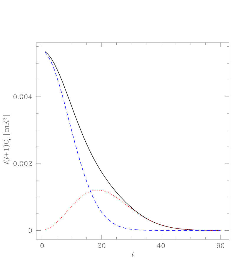
Figure 1: The angular power spectrum shown in this plot is used for all tests of the estimators presented in this section. It was chosen as a rough model for the DMR maps while remaining analytically tractable. The complete power spectrum, indicated by a solid line, is the sum of two contributions, namely a Harrison–Zeldovich spectrum normalized to $C_{10}=(7{\mu{\rm{K}}})^{2}$, convolved with a 7^∘ FWHM beam to mimick cosmic “signal” (dashed line), and random pixel noise (dotted line). In order to obtain a regular field and suppress noise the combined spectrum is smoothed with a Gaussian filter; its width for this particular example is 3^∘. Although the noise contribution has not been completely removed, it has been considerably reduced without affecting the signal too strongly. See Section 4.2 for a broader discussion of this issue.

Throughout this section, we will illustrate the application of our method on a particular random field. In order to stick to a simple, analytically tractable model, we generate a Gaussian random field. Its angular power spectrum $C_{\ell}$ is chosen to reproduce the salient features of the DMR sky maps. Hence, we start from angular components given by the formula

$$C_{\ell,\rm powerlaw}=C_{2}\frac{\Gamma\left(\ell+\frac{n-1}{2}\right)\Gamma\left(\frac{9-n}{2}\right)}{\Gamma\left(\ell+\frac{5-n}{2}\right)\Gamma\left(\frac{n+3}{2}\right)},$$ (17)

derived from a power–law spectrum $P(k)\propto{k^{n}}$ by bond:statistics, and smooth them with a Gaussian filter of 7^∘  FWHM to model the DMR beam. White noise with a fixed rms fluctuation level of $3{\mu{\rm{K}}}$ is then added to this “cosmic signal”; this is in practice done on the pixels in real space, but for comparison we may also evaluate the contribution to the angular power spectrum, which is

$$C_{\ell,\rm noise}=(3{\mu{\rm{K}}})^{2}$$ (18)

independent of $\ell$. Finally, a Gaussian smoothing kernel of variance $\omega^{2}$, given by

$$g_{\ell,\rm Gauss}=\exp\left(-{\textstyle\frac{1}{2}}\omega^{2}\ell(\ell+1)\right)$$ (19)

is applied to reduce the noise level, and to obtain a regular field. Note that the normalization factor $C_{2}$ in Equation (17) is directly related to the CMB quadrupole. As pointed out by gorski:onresults its particular value determined from the COBE DMR sky maps is highly dependent on the spectral index $n$; therefore it has become common usage to quote the multipole $C_{10}\approx(7{\mu{\rm{K}}})^{2}$ as a sufficiently spectrum independent normalization.

So the various contributions to the angular power spectrum $C_{\ell}$ for our example sum up to

$$C_{\ell}=g_{\ell,\rm Gauss}^{2}\left(C_{\ell,\rm powerlaw}g_{\ell,\rm beam}^{2}+C_{\ell,\rm noise}\right).$$ (20)

In Figure 1, the contributions of “signal” and noise are shown separately, and combined to the full spectrum, all after 3^∘ smoothing .

3.1 Estimators for a pixelized sky map

In order to estimate the Minkowski functionals from a discretized map we attempt to follow the prescription outlined by schmalzing:beyond for cubic grids in three–dimensional Euclidean space. Note that their first approach based on Crofton’s formula and counting of elementary cells is not viable since a strictly regular pixelization of the sphere does not exist. However, their second approach is based on averaging over invariants analogous to Equation (11), and can easily be adapted to the sphere. If the random field is sampled at $N$ pixels at locations ${\bf x}_{i}$ on the sphere, we only need to estimate the values ${\mathcal{I}}_{j}({\bf x}_{i})$ of the invariants from Equation (12) at each location.

3.1.1 Covariant derivatives

Using the well–known parametrization of the unit sphere through azimuth angle $\vartheta$ and polar angle $\varphi$ we can express the covariant derivatives at a point ${\bf x}=(\vartheta,\varphi)$ in terms of the partial derivatives;

$$\begin{split}u_{;\vartheta}&=u_{,\vartheta},\\ u_{;\varphi}&=\frac{1}{\sin\vartheta}u_{,\varphi},\\ u_{;\vartheta\vartheta}&=u_{,\vartheta\vartheta},\\ u_{;\vartheta\varphi}&=\frac{1}{\sin\vartheta}u_{,\vartheta\varphi}-\frac{\cos\vartheta}{\sin^{2}\vartheta}u_{,\varphi},\\ u_{;\varphi\varphi}&=\frac{1}{\sin^{2}\vartheta}u_{,\varphi\varphi}+\frac{\cos\vartheta}{\sin\vartheta}u_{,\vartheta}.\end{split}$$ (21)

The partial derivatives in turn are best calculated from the spherical harmonics expansion

$$u(\vartheta,\varphi)=\sum_{\ell=0}^{\infty}\sum_{m=-\ell}^{\ell}a_{\ell m}Y_{\ell m}(\vartheta,\varphi).$$ (22)

This is simply done by replacing the harmonic function $Y_{\ell m}$ with its appropriate partial derivative. Since the functions $Y_{\ell m}$ depend on $\varphi$ via sine and cosine functions only, the derivatives with respect to $\varphi$ can be obtained analytically. Partial derivatives with respect to $\vartheta$ are calculated via recursion formulae constructed by differentiating the recursion for the associated Legendre functions $P_{\ell}^{m}$, given for example by abramowitz:handbook.

3.1.2 Integrals over invariants

We still have to account for the finite number of sample points. This is done by replacing the delta function with a bin of finite width $\Delta$,

$$\delta(u-\nu)\approx\frac{1}{\Delta}{\bf 1}_{[-\Delta/2,+\Delta/2]}(u-\nu),$$ (23)

where ${\bf 1}_{A}$ is the indicator function of the set $A$, with ${\bf 1}_{A}(x)=1$ for $x\in{A}$, and ${\bf 1}_{A}(x)=0$ otherwise. The integrals summarized in Equation (11) are then estimated by summation over all pixels

$$v_{j}(\nu)\approx\frac{1}{N}\sum_{i=1}^{N}w_{i}{\mathcal{I}}_{j}({\bf x}_{i}).$$ (24)

For incomplete sky coverage we must restrict the average to the unmasked pixels. This problem is adressed in detail in Section 3.2.

3.2 Testing the estimators

3.2.1 Complete sky coverage

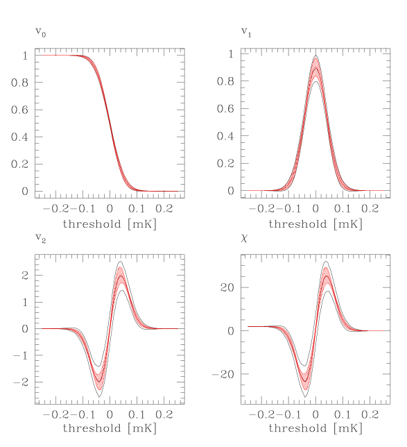
Figure 2: Minkowski functionals for the example used throughout this Section. The areas indicate the averages and $1\sigma$–fluctuations of an ensemble of 1,000 realizations computed on all 6,144 pixels of the DMR sky cube. The analytical expectation values in Equation (14) with parameters determined from the theoretical power spectrum via Equation (16) are almost exactly reproduced by the mean values (central lines). Fluctuations indicated by the shaded area are due to uncertainties in the parameter determination from a single map via Equation (15). They account for a large part of the overall fluctuations (empty area).

To begin with, let us look at the example without simulating the restrictions of incomplete sky coverage. Figure 2 shows the average Minkowski functionals of 1,000 realizations.

Looking at the general features of all curves, it can be seen that the area $v_{0}$ of hot spots decreases monotonically from the value of one at low threshold, when the whole sphere belongs to the excursion set, to a value of zero at high thresholds which are not passed by any of the pixels. The boundary length $v_{1}$ starts from a value of zero for a completely filled sphere. It reaches a maximum at intermediate thresholds, where the excursion set forms an interconnected pattern of patches and holes with a very long boundary. When the excursion set becomes emptier and emptier, the boundary length declines back to zero. For the random field shown in our example, the integrated geodesic curvature $v_{2}$ behaves largely similar to the Euler characteristic; the minor differences only become appreciable for fields with fewer features. Lastly, the Euler characteristic $\chi$ at low thresholds has a value of two for a closed sphere. With increasing threshold, the Euler characteristic declines to negative values as holes open in the excursion set and give a negative contribution. This downward trend gradually stops as individual hot spots emerge, so a minimum develops, and the Euler characteristic attains positive values. Finally, more and more hot spots fall below the growing threshold, so their number and hence the Euler characteristic decreases again, reaching a final value of zero.

A description of the individual curves can be found in the figure caption.

3.2.2 Uncertainties through incomplete sky coverage

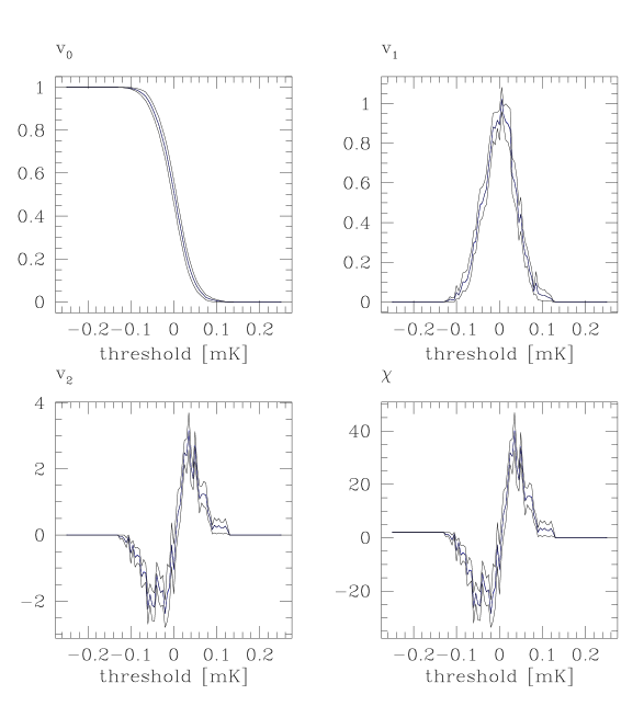
Figure 3: This plot shows the uncertainties due to a galactic cut. In order to separate them from fluctuations between different realizations in a ensemble (see Figure 2), we chose a single all–sky realization (central line) of the random field, and applied 1,000 straight cuts up to 30^∘  latitude with randomly varying orientation of the equatorial plane. It turns out that the uncertainties caused by this deterioration of statistics are at least as strong as ensemble fluctuation. However, the correct mean value is still reproduced (the mean and the true value conincide in the central line of the jagged area), so the estimator remains unbiased.

In practice, a data set will suffer from incomplete sky coverage. In order to estimate the uncertainties introduced solely by the galactic cut, we first contruct a single realization of the random field on the whole sky. The Minkowski functionals for this random field are calculated and roughly fit the analytical expectations, with fluctuations consistent with the areas shown in Figure 2. Then, we apply a series of straight galactic cuts with varying direction, but with constant width of $30{{}^{\circ}}$; this value reduces the number of pixels to exactly half the original value. Figure 3 shows a comparison of the true values for one field and the fluctuations introduced by the sample variance of the rotating cuts. Note that the smaller number of pixels does increase the uncertainties, but the average is not affected – the estimator remains unbiased.

3.2.3 Boundary effects

Figure 4: If the galactic cut is applied before smoothing the random field, as it should be done for real data, pixels in the vicinity of the galactic cut suffer from severe contamination. This leads to a visible bias in the estimated Minkowski functionals, particularly the integrated curvature $v_{2}$ and the Euler characteristic $\chi$, although the area $v_{0}$ and the circumference $v_{1}$ are also affected. The shaded area shows average and fluctuations for the all–sky map already presented in Figure 2, while the empty area with thicker contour and central line indicates the same quantities for the maps biased through the cut.

Figure 5: The biases demonstrated in Figure 4 can be removed by also smoothing the cut, and excluding points where the smoothed cut still reaches a certain level. In the example shown, this threshold was set to a very restrictive 1%; obviously the mean values agree completely. In practice, a level as high as 5% might still produce reliable results. Note that fluctuations have increased in comparison with the results obtained from all–sky maps, as already demonstrated in Figure 3.

Figure 6: The same quantities as in Figure 4 are compared in this plot, but with 200 random pixels excluded instead of the galactic cut. Contamination affects more pixels than in the case of a galactic cut – if a residue of 1% is allowed, 2,842 out of the original 6,144 pixels remain, compared to 3,189 for a galactic cut. However, the estimated Minkowski functionals are more robust.

The previous subsection dealt with a random field that was first realized on the whole sky, then smoothed with a Gaussian filter, and cut afterwards. In order to determine whether the galactic cut affects the estimators derived above, we use the COBE DMR pixels and the customized cut from the four–year data [Bennett et al.1996]. This time, we remove the pixels within the galactic cut before the smoothing kernel is applied.

It turns out that by using this procedure, which is actually the correct one for mimicking real data, the galactic cut severely affects the estimators, and leads to a systematic bias of as much as $1\sigma$. Figure 4 shows the unbiased results from all–sky maps already displayed in Figure 2, in comparison the biased result obtained with the naïvely applied estimator.

A straightforward procedure to remove these biases from the estimators is to further restrict the number of pixels to the ones that lie “far away” from the cut. In order to find them, we consider the indicator function of the cut itself, smooth it with the Gaussian filter, and consider the values at pixels outside the cut as their level of “contamination”. Now the sums from Equation (24) can be restricted to the pixels where the smoothed cut lies below a certain threshold. Figure 5 shows the results for an allowed level of 1%; in practice, even as much as 5% produces sufficiently unbiased estimates. Note that while the mean values agree completely after applying the correction, the variance of the estimators has increased, simply because fewer data points result in poorer statistics.

Apart from the galactic cut, point source contamination is another important source of incomplete sky coverage. Figure 6 shows the bias introduced by omitting 200 randomly scattered pixels. Obviously, the effect is much less pronounced compared to the realizations excluding the galactic cut; in fact the differences between the all–sky realizations and the restricted realizations are barely visible. Both the galactic cut and the random point cut affect roughly 3,000 of the 6,144 DMR pixels with a contribution of 1% or above, so at first sight our findings appear inconsistent. However, they can be explained with the prominent geometric features – namely, almost straight edges – in the galactic cut. These are missing in a random point distribution, so the errors remain smaller and average out.

4 Examples

4.1 The Earth

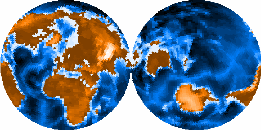
Figure 7: This map shows the earth’s topography at DMR resolution. The corresponding Minkowski functionals are displayed in Figure 8.

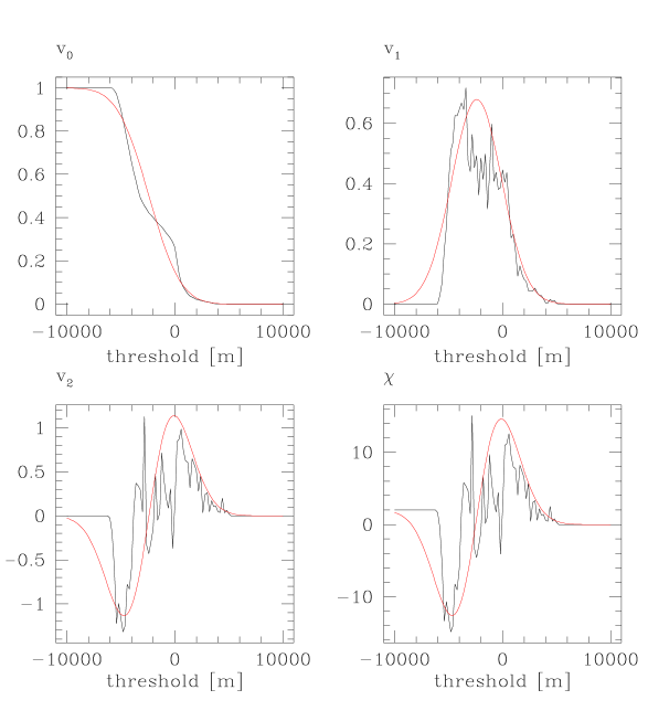
Figure 8: Minkowski functionals of the earth’s topography from the map in Figure 7 with a 1^∘  Gaussian filter applied. The resulting Minkowski functionals (jagged lines) look decidedly non–Gaussian; compare the analytical expectation values (smooth lines). Pronounced features in the Minkowski functional curves can be identified as corresponding to the main features of the earth’s topography, such as oceanic ridges, continents and mountain ranges. See the main text for details.

In order to provide a familiar example that does not look like a Gaussian random field even at DMR resolution, Figure 8 shows the Minkowski functionals of the earth’s topography. The map (see Figure 7) was constructed by binning the Etopo5 data into the DMR pixels.

The curves reveal a number of characteristic features. All functionals experience a fairly sharp change at a depth between 6,000m and 5,000m, which is roughly the average depth of the seafloor. A peak of several 1,000m width and almost constant height of the boundary length $v_{1}$, and a corresponding minimum in the Euler characteristic $\chi$ indicate the rise of the oceanic ridges. From 3,000m below sea level to slightly positive elevations, the boundary length remains largely constant, as the continental shelfs rise from the oceans; meanwhile, the Euler characteristic fluctuates with the disappearance of the oceanic ridges, and the opening of shallower, marginal parts of the oceans such as the Mediterranean, the Carribean sea or the Artic sea. Most of the land mass does not rise beyond 1,000m, so all Minkowski functionals gradually decline after this height; a few small peaks in the Euler characteristic may be – cautiously – identified with Antarctica, the Rocky Mountains, the Andes, and the Himalaya.

4.2 How smoothing leads to noise reduction

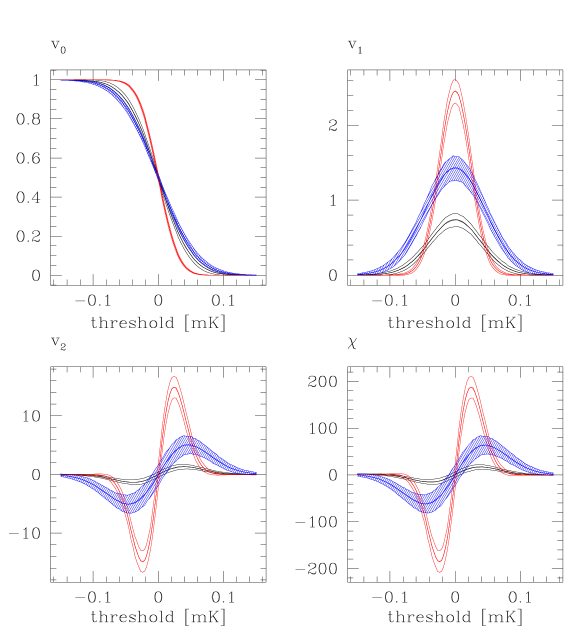
Figure 9: Signal (shallow curves, empty area), noise (sharply peaked curves, empty area) and combination of both (shaded area) at 2^∘ smoothing. At this scale, the noise contribution contains far more features than the signal. Moreover, they are strong enough to persist when distributed over the whole range of the signal. Hence the combination of signal and noise displays a completely different morphology from the pure signal contribution.

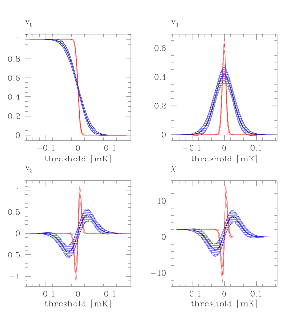
Figure 10: Signal (shallow curves, empty area), noise (sharply peaked curves, empty area) and combination of both (shaded area) of the same random field as in Figure 9, but at 8^∘ smoothing. Although the pure noise map still features roughly two dozen extrema, their amplitude has been reduced to such extent that the pure signal is hardly affected when combined with the noise.

In order to obtain a regular field, and to reduce the level of the additive noise present in the data, it is necessary to apply a smoothing kernel to the data before calculating the Minkowski functionals. Usually, the choice of a particular width is largely arbitrary. Here we show the example introduced in Section 4 with different degrees of smoothing applied to illustrate the behaviour of Minkowski functionals in the presence of noise.

The situation for 2^∘  smoothing, where noise still makes an appreciable contribution, is shown in Figure 9. The surface area $v_{0}$ is much less affected than the other Minkowski functionals; this is due to the fact that noise is incoherent and forms comparatively small hot and cold spots. However, these spots are almost as intense as the signal contribution, as can be seen from the almost equal width of all curves, and far more numerous – the Euler characteristic for the noise field alone reaches a maximum of the order of 200. Even though the extrema in the pure noise maps are spread out over the whole range of thresholds when added to the signal, and hence their number at a specific threshold decreases, their contribution is still sufficiently high to make the signal appear completely different compared to the combination of signal and noise.

In Figure 10, where the results for 8^∘ smoothing are displayed, noise is almost completely invisible in comparison to the signal. Only about two dozen extrema of either kind (compare the extrema of the Euler characteristic) remain, but since they have become extremely shallow, their contribution is not significant any more; the pure signal and the combination of signal and noise differ only marginally. Unfortunately, at a resolution of 8^∘ the remaining signal does not carry too much cosmological information.

With this example, the behaviour of Minkowski functionals under filtering at different scales has only been hinted at. The two filter widths of 2^∘  and 8^∘  are chosen to show two extremal possibilities, namely total dominance of noise and total reduction of noise. In practice, the intermediate value of 3^∘  turns out to give good enhancement of signal, while preserving small–scale information as well.

4.3 Analysis of the COBE DMR four–year data

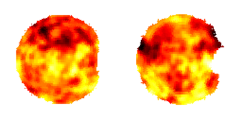
Figure 11: This panel shows the four–year data from the COBE DMR 53GHz channel, with a customized galactic cut and a smoothing filter of 3^∘ width applied. Figure 12 displays the corresponding Minkowski functionals calculated both from this map, and from the all–sky map with galactic signal dominating.

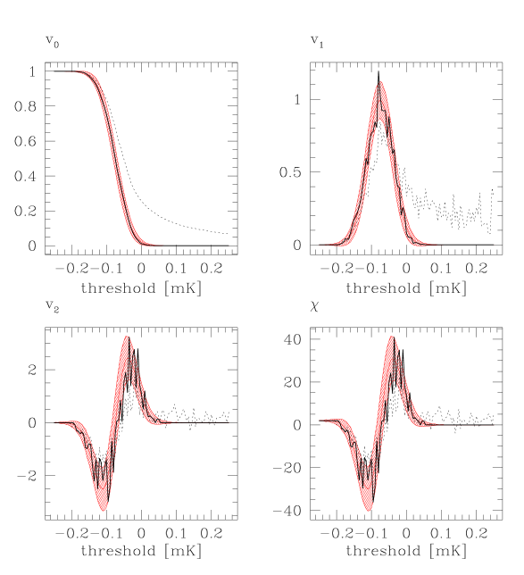
Figure 12: Minkowski functionals of the four–year COBE DMR map in the 53GHz channel. As expected, the full map of 6,144 pixels (dashed line) is severely affected by galactic emission; this results in long tails for all Minkowski functionals. Using a galactic cut, the functionals determined from the map (solid line) become consistent with a stationary Gaussian random field. The shaded area indicates the mean and variance of 1,000 realizations of a Gaussian random field with Harrison–Zel’dovich spectrum and pixel noise; normalizations were chosen to reproduce the parameters $\mu$, $\sigma$ and $\tau$ determined from the data via Equation (15).

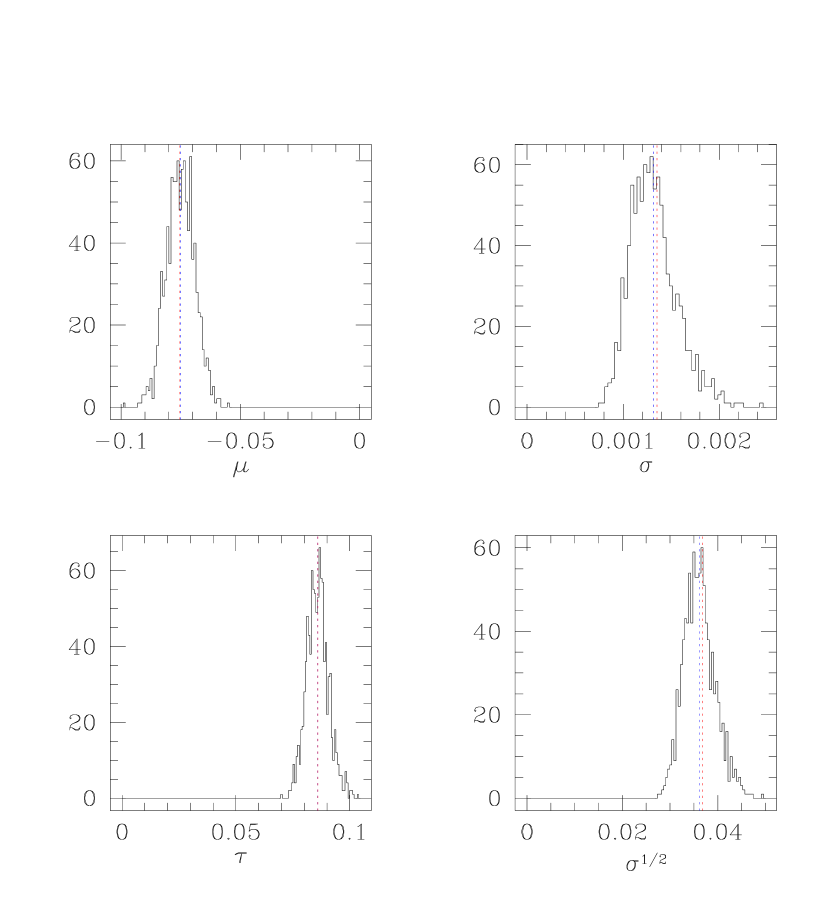
Figure 13: Uncertainties in the parameter estimates. Parameters were determined from each of the 1,000 simulated DMR maps, and binned into histograms. In order to give an idea of the amount of uncertainty, the range is extended to include zero in all plots. Obviously, the fluctuations are still fairly large in comparison to the mean value; to be precise, the relative rms fluctuation is roughly 8% for $\mu$, almost 6% for $\tau$, and more than 9% for $\sqrt{\sigma}$.

As a last example, let us take a look at data that are both real and cosmologically relevant. Figure 11 shows a map of the microwave sky as seen at 53GHz by the COBE satellite after four years of observing [Bennett et al.1996]. The data are restricted to 3,189 pixels receiving less than 1% from a smoothed galactic cut, when a Gaussian filter of 3^∘  width is applied. Figure 12 displays the corresponding Minkowski functionals. Obviously, the analysis carried out on all 6,144 pixels is dominated by galactic emission, while the field with the galactic cut applied is consistent with the assumption of a stationary Gaussian random field. However, this result should be considered a illustration of the method rather than conclusive evidence, since our brief analysis probes a scale of roughly 4^∘  (given by the squared sum of 2.6^∘ pixel size and 3^∘ Gaussian filter width).

As stated above, considerable uncertainties are introduced through the estimates of the parameters $\mu$, $\sigma$ and $\tau$ entering the analytical expectation values for the Minkowski functionals of a Gaussian random field. In order to make this statement more quantitative, Figure 13 summarizes the parameters determined from the 1,000 mock realizations used for the shaded area in Figure 12. Relative errors for the relevant parameters lie in the range of five to ten per cent, which is not too bad considering that little more than 3,000 data points enter our analysis.

5 Summary and outlook

We have introduced Minkowski functionals of isotemperature contours as a novel tool to characterize the morphology of Cosmic Microwave Background sky maps.

Using the framework of integral geometry in curved spaces, we were able to clarify the geometric interpretations of all Minkowski functionals in two dimensions. Writing all Minkowski functionals as spatial averages over invariants formed from covariant derivatives, lead to simple formulae for estimators applicable to pixelized sky maps, including a straightforward prescription for dealing with incomplete sky coverage. Finally, analytical formulae for all Minkowski functionals of the excursion sets of a Gaussian random field could be provided.

The study of a simplified yet realistic model served to test the theoretically derived estimators in their application to simulated CMB sky maps. Among other tests, we checked whether the estimators remain unbiased when incomplete data is smoothed over the edge of a galactic cut, and found a prescription to deal with this problem while preserving as much information as possible.

A number of examples provided further illustrations of the application of our method, and showed how to interpret the calculated Minkowski functionals in close touch with the analyzed data sets. The analysis of the earth’s topography using Minkowski functionals explained how to cast the bridge from the behaviour of the Minkowski functional curves to outstanding features in the underlying random field. As a more serious application, we showed the successive reduction of noise through Gaussian smoothing with increasing filter width – in the end, a complete removal of the noise effects from the Minkowski functionals is obtained. The final example briefly analyzed a COBE DMR map, with the not particularly surprising result that the field is consistent with a Gaussian random field on degree scales.

Minkowski functionals combine the benefits of a sound mathematical framework and well–understood analytical possibilities with intuitive interpretations and easy applicability to real data. Hence they qualify as a method suited to study the Microwave sky at higher resolution, where the obstacle of poor statistics should not be an issue. While experiments to obtain high–resolution maps of large regions of the sky are still under development (bersanelli:cobrassamba, bennett:map), testing the Minkowski functionals on simulations is an important task for the future. In particular, we need to assess their power to detect non–Gaussianity, and find the possibilities to estimate cosmological parameters from Minkowski functionals in an approach complementary to the power spectrum analysis.

Appendix A Geodesic curvature of an isodensity contour

Consider a scalar field $u$ on a two–dimensional differentiable manifold ${\mathfrak{M}}$. We wish to calculate the geodesic curvature of the isodensity contour passing through a point ${\bf x}_{0}\in{\mathfrak{M}}$. To do this, we use a procedure outlined by koenderink:scalespace. In a sufficiently small neighbourhood we can always find an explicit parametrization ${\bf x}(t)$ of the isodensity contour, with ${\bf x}(t=0)={\bf x}_{0}$. The corresponding threshold is $\nu=u({\bf x}_{0})$, and therefore the contour is implicitly described by

$$u({\bf x}(t))=\nu.$$ (25)

It follows by covariant differentiation with respect to the parameter $t$ that

$$u_{;i}\dot{x}_{i}=0$$ (26)

must hold. So we can choose the tangent vector

$$\dot{x}_{i}=\epsilon_{ij}u_{;j}.$$ (27)

Actually this choice is not unique and reflects the freedom of parametrization; however, care must be taken to orient the tangent vector towards regions of lower values of $u$. Differentiating Equation (25) a second time we obtain

$$u_{;ij}\dot{x}_{i}\dot{x}_{j}+u_{;k}\ddot{x}_{k}=0$$ (28)

whence we can now evaluate the geodesic curvature $\kappa$ of the isodensity contour via the well–known formula

$$\kappa=\frac{\dot{x}_{i}\epsilon_{ij}\ddot{x}_{j}}{(\dot{x}_{k}\dot{x}_{k})^{3/2}}.$$ (29)

As our final result we obtain

$$\kappa=\frac{2u_{;1}u_{;2}u_{;12}-u_{;1}^{2}u_{;22}-u_{;2}^{2}u_{;11}}{(u_{;1}^{2}+u_{;2}^{2})^{3/2}}.$$ (30)

Note that this formula contains the covariant derivatives of $u$ and therefore holds for any manifold ${\mathfrak{M}}$, regardless of the metric.

Appendix B Average Minkowski functionals for a Gaussian random field

Isodensity contours of a Gaussian random field have been excessively studied ever since the works of doroshkevich:gauss on the genus. Comprehensive overviews can be found in the book by adler:randomfields or the famous BBKS paper [Bardeen et al.1986]. A highly instructive derivation of the average values for all Minkowski functionals in arbitrary dimension can be found in [Tomita1990]. Nevertheless, we will outline a calculation directly related to our approach to the numerical evaluation.

A homogeneous Gaussian random field $u$ with zero mean on a two–dimensional manifold ${\mathfrak{M}}$ is fully described by correlation function $\xi(r)$. We wish to calculate the average Minkowski functionals $v_{j}(\nu)$ of an isodensity contour to the threshold $\nu$. Because of Equations (11) and (12) it is sufficient to know the joint probability distribution of the field’s value itself and the derivatives up to second order at some fixed point.

According to adler:randomfields these six variables are jointly Gaussian distributed. Hence their probability distribution function can be written in concise form by arranging them into a vector ${\bf u}=\left(u,u_{;1},u_{;2},u_{;11},u_{;22},u_{;12}\right)$; we have

$$P({\bf u})=\frac{1}{\sqrt{(2\pi)^{d}\det{\boldsymbol{\sigma}}}}\exp\left(-\frac{1}{2}{\bf u}^{T}{\boldsymbol{\sigma}}^{-1}{\bf u}\right),$$ (31)

with the covariance matrix ${\boldsymbol{\sigma}}$ taken from tomita:statistics

$${\boldsymbol{\sigma}}=\left(\begin{array}[]{cccccc}\sigma&0&0&-\tau&-\tau&0\\ 0&\tau&0&0&0&0\\ 0&0&\tau&0&0&0\\ -\tau&0&0&\upsilon&\upsilon/3&0\\ -\tau&0&0&\upsilon/3&\upsilon&0\\ 0&0&0&0&0&\upsilon/3\end{array}\right).$$ (32)

Note that the parameters $\sigma=\xi(0)$, $\tau=|\xi^{\prime\prime}(0)|$ and $\upsilon=\xi^{\prime\prime\prime\prime}(0)$ all depend on the correlation function $\xi(r)$.

Now we can perform the averages

$$\begin{split}v_{0}(\nu)&=\int{\rm d}{\bf u}P({\bf u})\Theta(u-\nu)\\ v_{1}(\nu)&=\int{\rm d}{\bf u}P({\bf u})\delta(u-\nu)\sqrt{u_{;1}^{2}+u_{;2}^{2}}\\ v_{2}(\nu)&=\int{\rm d}{\bf u}P({\bf u})\delta(u-\nu)\frac{2u_{;1}u_{;2}u_{;12}-u_{;1}^{2}u_{;22}-u_{;2}^{2}u_{;11}}{u_{;1}^{2}+u_{;2}^{2}}\end{split}$$ (33)

by straightforward integration, and have recovered the results of tomita:statistics in two dimensions

$$\begin{split}v_{0}(\nu)&={\textstyle\frac{1}{2}}-{\textstyle\frac{1}{2}}\Phi\left(\frac{\nu}{\sqrt{2\sigma}}\right),\\ v_{1}(\nu)&={\textstyle\frac{\pi}{4}}\frac{\lambda}{\sqrt{2\pi}}\exp\left(-\frac{\nu^{2}}{2\sigma}\right),\\ v_{2}(\nu)&=\frac{\lambda^{2}\nu}{\sqrt{2\pi\sigma}}\exp\left(-\frac{\nu^{2}}{2\sigma}\right).\end{split}$$ (34)

As stated in the main text, the result depends on only two parameters, namely

$$\sigma=\xi(0),\qquad\lambda=\sqrt{\dfrac{|\xi^{\prime\prime}(0)|}{2\pi\xi(0)}}.$$ (35)

References

- [\citefmtAbramowitz & Stegun1970] Abramowitz, M. X. & Stegun, I. A., Handbook of mathematical functions, 9th ed., Dover Publications, New York, 1970.
- [\citefmtAdler1981] Adler, R. J., The geometry of random fields, John Wiley & Sons, Chichester, 1981.
- [\citefmtAllendoerfer & Weil1943] Allendoerfer, C. B. & Weil, A., Trans. Amer. Math. Soc. 53 (1943), 101–129.
- [\citefmtBardeen et al.1986] Bardeen, J. M., Bond, J. R., Kaiser, N., & Szalay, A. S., Ap. J. 304 (1986), 15–61.
- [\citefmtBennett et al.1995] Bennett, C. L., Hinshaw, G., Jarosik, N. C., Mather, J., Meyer, S. S., Page, L., Skillman, D., Spergel, D. N., Wilkinson, D. T., & Wright, E. L., Bull. American Astron. Soc. 187 (1995), no. 71.09, 1385.
- [\citefmtBennett et al.1996] Bennett, C. L., Banday, A., Górski, K. M., Jackson, P. D., Keegstra, P. B., Kogut, A., Smoot, G. F., Wilkinson, D. T., & Wright, E. L., Ap. J. Lett. 464 (1996), L1–L4.
- [\citefmtBersanelli et al.1996] Bersanelli, M., Bouchet, F. R., Efstathiou, G., Griffin, M., Lamarre, J. M., Mandolesi, N., Norgaard-Nielsen, H. U., Pace, O., Polny, J., Puget, J. L., Tauber, J., Vittorio, N., & Volonté, S., COBRAS/SAMBA. A mission dedicated to imaging the anisotropies of the cosmic microwave background. Report on the phase A study, European Space Agency, February 1996.
- [\citefmtBlaschke1936] Blaschke, W., Integralgeometrie. Erstes Heft, Bernd G. Teubner, Leipzig, Berlin, 1936.
- [\citefmtBond & Efstathiou1987] Bond, J. R. & Efstathiou, G., Mon. Not. Roy. Astron. Soc. 226 (1987), 655–687.
- [\citefmtChern1944] Chern, S.-S., Ann. of Math. 45 (1944), 747–752.
- [\citefmtColes & Barrow1987] Coles, P. & Barrow, J. D., Mon. Not. Roy. Astron. Soc. 228 (1987), 407–426.
- [\citefmtColes1988] Coles, P., Mon. Not. Roy. Astron. Soc. 234 (1988), 509–531.
- [\citefmtColley et al.1996] Colley, W. N., Gott III, J. R., & Park, C., Mon. Not. Roy. Astron. Soc. 281 (1996), L82–L84.
- [\citefmtDoroshkevich1970] Doroshkevich, A. G., Astrophysics 6 (1970), 320–330.
- [\citefmtGórski et al.1994] Górski, K. M., Hinshaw, G., Banday, A. J., Bennett, C. L., Wright, E. L., Kogut, A., Smoot, G. F., & Lubin, P. M., Ap. J. Lett. 430 (1994), L89–L92.
- [\citefmtGórski et al.1996] Górski, K. M., Banday, A. J., Bennett, C. L., Hinshaw, G., Kogut, A., Smoot, G. F., & Wright, E. L., Ap. J. Lett. 464 (1996), L11–L16.
- [\citefmtGott III et al.1990] Gott III, J. R., Park, C., Juszkiewicz, R., Bies, W. E., Bennett, D. P., Bouchet, F. R., & Stebbins, A., Ap. J. 352 (1990), 1–14.
- [\citefmtHadwiger1957] Hadwiger, H., Vorlesungen über Inhalt, Oberfläche und Isoperimetrie, Springer Verlag, Berlin, 1957.
- [\citefmtHinshaw et al.1995] Hinshaw, G., Banday, A. J., Bennett, C. L., Górski, K. M., & Kogut, A., Ap. J. Lett. 446 (1995), L67–L70.
- [\citefmtHinshaw et al.1996] Hinshaw, G., Banday, A. J., Bennett, C. L., Górski, K. M., Kogut, A., Lineweaver, C. H., Smoot, G. F., & Wright, E. L., Ap. J. Lett. 464 (1996), L25–L28.
- [\citefmtKerscher et al.1997a] Kerscher, M., Schmalzing, J., Buchert, T., & Wagner, H., Astron. Astrophys. (1997), accepted, astro-ph/9704028.
- [\citefmtKerscher et al.1997b] Kerscher, M., Schmalzing, J., Retzlaff, J., Borgani, S., Buchert, T., Gottlöber, S., Müller, V., Plionis, M., & Wagner, H., Mon. Not. Roy. Astron. Soc. 284 (1997), 73–84.
- [\citefmtKogut et al.1995] Kogut, A., Banday, A. J., Bennett, C. L., Hinshhaw, G., Lubin, P. M., & Smoot, G. F., Ap. J. Lett. 439 (1995), L29–L32.
- [\citefmtKogut et al.1996] Kogut, A., Banday, A. J., Bennett, C. L., Górski, K. M., Hinshaw, G., Smoot, G. F., & Wright, E. L., Ap. J. Lett. 464 (1996), L29–L34.
- [\citefmtLuo & Schramm1993] Luo, X. & Schramm, D. N., Ap. J. 408 (1993), 33–42.
- [\citefmtMecke et al.1994] Mecke, K. R., Buchert, T., & Wagner, H., Astron. Astrophys. 288 (1994), 697–704.
- [\citefmtMinkowski1903] Minkowski, H., Mathematische Annalen 57 (1903), 447–495.
- [\citefmtPenzias & Wilson1965] Penzias, A. A. & Wilson, R. W., Ap. J. 142 (1965), 419–421.
- [\citefmtPompilio et al.1995] Pompilio, M. P., Bouchet, F. R., Murante, G., & Provenzale, A., Ap. J. 449 (1995), 1–8.
- [\citefmtSantaló1976] Santaló, L. A., Integral geometry and geometric probability, Addison–Wesley, Reading, MA, 1976.
- [\citefmtSchmalzing & Buchert1997] Schmalzing, J. & Buchert, T., Ap. J. Lett. 482 (1997), L1–L4.
- [\citefmtSchneider1978] Schneider, R., Ann. Math. pura appl. 116 (1978), 101–134.
- [\citefmtSchneider1993] Schneider, R., Convex bodies: the Brunn–Minkowski theory, Cambridge University Press, Cambridge, 1993.
- [\citefmtSmoot et al.1994] Smoot, G. F., Tenorio, L., J., B. A., Kogut, A., Wright, E. L., Hinshaw, G., & Bennett, C. L., Ap. J. 437 (1994), 1–11.
- [\citefmtStebbins1988] Stebbins, A., Ap. J. 327 (1988), 584–614.
- [\citefmtter Haar Romeny et al.1991] ter Haar Romeny, B. M., Florack, L. M. J., Koenderink, J. J., & Viergever, M. A., in: Lecture Notes in Computer Science, Vol. 511, Springer Verlag, Berlin, 1991, pp. 239–255.
- [\citefmtTomita1986] Tomita, H., Progr. Theor. Phys. 76 (1986), 952–955.
- [\citefmtTomita1990] Tomita, H., in: Formation, dynamics and statistics of patterns (Kawasaki, K., Suzuki, M., & Onuki, A., eds.), Vol. 1, World Scientific, 1990, pp. 113–157.
- [\citefmtTorres et al.1995] Torres, S., Cayón, L., Martínez–González, E., & Sanz, J. L., Mon. Not. Roy. Astron. Soc. 274 (1995), 853–857.
- [\citefmtTorres1994] Torres, S., Ap. J. Lett. 423 (1994), L9–L12.