Minkowski Functional Description of Microwave Background Gaussianity

Abstract

A Gaussian distribution of cosmic microwave background temperature fluctuations is a generic prediction of inflation. Upcoming high-resolution maps of the microwave background will allow detailed tests of Gaussianity down to small angular scales, providing a crucial test of inflation. We propose Minkowski functionals as a calculational tool for testing Gaussianity and characterizing deviations from it. We review the mathematical formalism of Minkowski functionals of random fields; for Gaussian fields the functionals can be calculated exactly. We then apply the results to pixelized maps, giving explicit expressions for calculating the functionals from maps as well as the Gaussian predictions, including corrections for map boundaries, pixel noise, and pixel size and shape. Variances of the functionals for Gaussian distributions are derived in terms of the map correlation function. Applications to microwave background maps are discussed.

I Introduction

The Cosmic Microwave Background (CMB) provides the earliest obtainable direct information about the Universe. Upcoming experiments (see, e.g., MAP 1996; Planck 1996) will map CMB temperature and polarization fluctuations with unprecedented sensitivity and angular resolution. Recent analyses have demonstrated that such maps contain a wealth of cosmological information, allowing a high-precision determination of the fundamental cosmological parameters (Jungman et al. 1996a,b; Zaldarriaga et al. 1997; Bond et al. 1997; Kamionkowski and Kosowsky 1997) and a clean separation of inflationary and topological defect models of structure formation (Pen et al. 1997; Hu and White 1997). These exciting prospects will keep the CMB at the forefront of cosmology for the coming decade.

Most theoretical and experimental results to date have focussed on the angular power spectrum of the CMB. If the temperature and polarization fluctuations are Gaussian, then the power spectrum contains all available information about the fluctuations; even if the fluctuations depart from Gaussian, the power spectrum is still a valuable and fundamental characterization of the fluctuations. For experiments on large angular scales, notably the DMR maps from the COBE satellite (Bennett et al. 1996), homogeneity of the Universe essentially guarantees a Gaussian anisotropy distribution via the central limit theorem since the experiment only probes scales outside of the causal horizon at last scattering (for a relevant discussion, see Scherrer and Schaefer 1995). Probes of the anisotropies at resolutions of one degree and smaller hold the possibility of uncovering non-Gaussian signatures. Theoretically, Gaussian fluctuations are well motivated, as inflation generically produces Gaussian-distributed scalar and tensor metric perturbations (Guth and Pi 1982; Starobinskii 1982; Hawking 1982; Bardeen et al. 1983), although this prediction can be circumvented in some unusual models (Allen et al. 1987; Salopek et al. 1989). Measurement of Gaussian fluctuation statistics at all angular scales would clear a major hurdle for inflation; conversely, discovery of cosmological non-Gaussianity would cast strong doubt on the inflationary scenario. If the Universe is not described by an inflationary model, non-Gaussianity will be an important clue in unraveling the nature of the primordial density perturbations.

A variety of techniques have been applied so far to test for Gaussianity in CMB data, primarily COBE maps. The two-point correlation function is equivalent to the fluctuation power spectrum. In principle, the higher-order correlation functions provide a complete test of Gaussianity; indeed, a Gaussian distribution can be defined as one in which the odd (3-point, 5-point, etc.) correlations are all zero, while the even correlation functions all factorize into products of two-point functions. Kogut et al. (1996), following earlier analysis of the 2-year maps (Smoot et al. 1994) and theoretical work (Luo and Schramm 1993; Luo 1994), have calculated certain 3-point functions for the COBE 4-year maps, finding the data consistent with zero (Gaussian). A drawback of analyzing N-point correlation functions is that computation time becomes prohibitive for higher-point functions unless restricted to specific fixed configurations of points, which provides a weaker test of Gaussianity than the most general case. Also, higher-point analysis of maps with complicated boundaries presents further difficulties.

Another, more heuristic statistic is the two-point correlation of temperature extrema (peaks and valleys), introduced by Bond and Efstathiou (1987), who provide analytic approximations to the correlation function for noiseless Gaussian random fields. The COBE 4-year maps are also consistent with Gaussianity for this statistic (Kogut et al. 1996). Finally, substantial attention has been focussed on the topological genus of temperature contours (Coles, 1988; Gott et al. 1990; Smoot et al. 1994; Torres et al. 1995; Colley et al. 1996; Kogut et al. 1996). The genus, as will be discussed below, is equivalent to one of the three Minkowski functionals for a two-dimensional map.

In this paper we concentrate on the set of statistics known as Minkowski functionals (Minkowski 1903). A general theorem of integral geometry states that all properties of a $d$-dimensional convex set (or more generally, a finite union of convex sets) which satisfy translational invariance and additivity (called morphological properties) are contained in $d+1$ numerical values (Hadwiger, 1956 and 1959). For a pixelized temperature map $T({\bf n})$ (or, e.g., a density field), we consider the excursion sets of the map, defined as the set of all map pixels with value of $T$ greater than some threshold $\nu$ (see, e.g., Weinberg et al. 1987; Melott 1990). Then the three functionals of these excursion sets completely describe the morphological properties of the underlying temperature map $T({\bf n})$. In two and three dimensions, the Minkowski functionals have intuitive geometric interpretations. The key point relevant for this paper is that the Minkowski functionals can be calculated exactly for an underlying Gaussian field (Tomita 1990). Thus they provide a natural set of statistical tests for Gaussianity. Recently, Buchert and collaborators have introduced Minkowski functionals into the cosmological literature, primarily in the context of three-dimensional point distributions applied to galaxy surveys (Mecke et al. 1994; Buchert 1995; Kerscher et al. 1997).

For a two-dimensional map, the three Minkowski functionals correspond geometrically to the total fractional area of the excursion set, the boundary length of the excursion set per unit area, and the Euler characteristic per unit area (equivalent to the topological genus). The area (Coles 1988, Ryden et al. 1989) and the genus (mentioned above) have been previously considered in the context of microwave background temperature maps, but not in the unified formal context of the Minkowski functionals. The additivity property, previously not exploited, allows an evaluation of the standard errors in estimating the functionals from a map, rather than resorting to Monte Carlo simulations as in previous work (Scaramella and Vittorio 1991; Torres et al. 1995; Kogut et al. 1996). A second property, given by the principle kinematic formulas, provides a recipe for incorporating arbitrary map boundaries in a straightforward way, a valuable advantage when analyzing upcoming maps with irregular portions of the sky cut out to eliminate contamination from foreground emission.

This paper applies the formalism of Minkowski functionals to pixelized two-dimensional maps as a test of Gaussianity; the results will be directly applicable to temperature maps of the microwave background. In Sec. II, we present an overview of Minkowski functionals of continuous fields and explicate their relevant mathematical properties. Section III then considers the related case of Minkowski functionals on a lattice, or equivalently of a pixelized map. We give explicit formulas for variances of the functionals and corrections for boundaries. We also give explicit calculational algorithms for different pixelization schemes. Section IV addresses the issue of Gaussianity, giving the explicit forms for the Minkowski functionals for underlying Gaussian statistical distributions. Pixelization introduces corrections to the Gaussian functionals in the smooth case, which we derive as power series in the pixel size. Finally, we conclude in section V with a discussion of various issues related to analyzing maps, including noise, smoothness, and numerical efficiency.

II Review of Minkowski Functionals

We are interested in characterizing the morphological properties of microwave background maps, the properties of the map which are invariant under translations and rotations and which are additive. For example, the area of the map which is above a certain temperature threshold is a morphological characteristic. The branch of mathematics known as integral geometry provides a natural tool for this characterization, known as the Minkowski functionals (or quermassintegrals). In this section we give a brief review of Minkowski functionals and summarize their basic properties. For further details and general mathematical background, see Weil (1983) or Stoyan et al. (1987).

Consider a convex set $K$ in ${\bf R}^{d}$. The parallel set of distance $r$ to $K$ is the set

$$K_{r}=\bigcup_{k\in K}b(k,r),$$ (1)

where $b(k,r)$ is the closed ball of radius $r$ centered at the point $k$. A relation called the Steiner formula can be taken as the definition of the Minkowski functionals $W_{i}$:

$$V(K_{r})=\sum_{i=0}^{d}{d\choose i}W_{i}(K)r^{i},$$ (2)

where $V$ denotes the ($n$-dimensional) volume. For low-dimensional spaces, the Minkowski functionals can be expressed simply in terms of the geometrical quantities length $\ell(K)$ (for $d=1$), area $A(K)$ and boundary length $L(K)$ (for $d=2$), and volume $V(K)$, surface area $S(K)$, and mean breadth ${\bar{b}}(K)$ (for $d=3$):

$$W_{0}(K)=\ell(K),\qquad W_{1}(K)=2\qquad(d=1);$$ (4)

$$W_{0}(K)=A(K),\qquad W_{1}(K)={\frac{1}{2}}L(K),\qquad W_{2}(K)=\pi\qquad(d=2);$$ (5)

$$W_{0}(K)=V(K),\qquad W_{1}(K)={\frac{1}{3}}S(K),\qquad W_{2}(K)={\frac{2\pi}{3}}{\bar{b}}(K),\qquad W_{3}(K)={\frac{4\pi}{3}}\qquad(d=3).$$ (6)

The Steiner formula can also be generalized to the other Minkowski functionals besides volume as

$$W_{j}(K_{r})=\sum_{i=0}^{d-j}{d-j\choose i}W_{i+j}(K)r^{i}.$$ (7)

The motivation for using the Minkowski functionals for characterizing morphology is the following completeness theorem of Hadwiger (1959). For ${\cal K}^{d}$ the class of convex, compact sets in ${\bf R}^{d}$, consider a continuous map $T:{\cal K}^{d}\rightarrow{\bf R}$ which satisfies the properties of motion invariance and additivity:

$$T(gK)=T(K)\,\,\,\forall K\in{\cal K}^{d},\,\,g\in G_{d},$$ (8)

where $G_{d}$ is the group of rigid motions in $d$ dimensions (i.e., rotations and translations); and

$$T(K_{1}\cup K_{2})+T(K_{1}\cap K_{2})=T(K_{1})+T(K_{2})$$ (9)

for $K_{1},\,K_{2}\in{\cal K}^{n}$ with $K_{1}\cup K_{2}\in{\cal K}^{d}$. Then $T$ can be expressed as a linear combination of the Minkowski functionals:

$$T(K)=\sum_{i=0}^{d}\alpha_{i}W_{i}(K),\quad\alpha_{i}\in{\bf R}.$$ (10)

In other words, all of the morphological information about a convex body is contained in the Minkowski functionals.

In the following sections, we will not be concerned with characterizing a single convex set but rather a finite union of convex sets (i.e. map pixels), or in mathematical terms, sets which are elements of the convex ring ${\cal R}^{n}$ (Hadwiger 1956 and 1959). In two dimensions, the area and boundary length functionals have obvious generalizations to the convex ring, while the third functional becomes the Euler-Poincare characteristic. The Hadwiger characterization theorem, Eq. (10), generalizes to the convex ring. In this paper, we will find it convenient to work with a different normalization of the functionals, given by

$$M_{i}(K)\equiv\frac{\omega_{d-i}}{\omega_{d}\omega_{i}}W_{i}(K),$$ (11)

where $\omega_{d}=\pi^{d/2}/\Gamma(1+d/2)$ is the volume of the unit ball in $d$ dimensions. The three functionals of an element of ${\cal R}^{2}$ are then

$$M_{0}=A,\qquad M_{1}=\frac{1}{2\pi}L,\qquad M_{2}=\frac{1}{\pi}\chi,$$ (12)

where $\chi$ is the Euler characteristic.

Another set of useful relations are the so-called principle kinematic formulae (Hadwiger 1957, Santalo 1976), which can be written concisely as (Mecke et al. 1994)

$$\int_{G_{d}}M_{i}(K_{1}\cap gK_{2})dg=\sum_{j=0}^{i}{i\choose j}M_{i-j}(K_{2})M_{j}(K_{1}).$$ (13)

The integral is over the group of motions, formally with an invariant Haar measure $dg$. This formula describes the set $K_{1}$ through its intersections with a test body $K_{2}$ in random orientations.

To analyze a map in terms of Minkowski functionals, we consider the excursion sets of the map, the map subset which exceeds a fixed threshold value. The threshold is treated as an independent variable on which the Minkowski functionals of the excursion set depend. The three functionals of interest are (up to irrelevant constant factors, cf. Eq. (5)) the area of the excursion set $A$, its boundary length $L$, and its Euler-Poincare characteristic $\chi$ (or equivalently, its topological genus). The following section discusses in detail how to construct a discrete version of these functionals, applicable to a pixelized map.

III Minkowski functionals on a lattice

The method of analysis proposed in this paper consists of comparing the values of the Minkowski functionals $M_{i}$ calculated from an experimentally obtained map with the theoretical predictions for the expectation values and variances of $M_{i}$ on Gaussian distributions. Carrying out this program requires calculation of the Minkowski functionals from given maps, properly taking into account the boundary of the observed region and the effect of pixelization.

This section presents the necessary formalism for the analysis of Minkowski functionals on a lattice. Rather than treat pixelized maps as approximations to the “true” continuous temperature field, we apply the formalism of the Minkowski functionals directly to random functions on discrete lattices (for extensive mathematical background, see Serra 1982). Although some elements of this consideration are present in the literature (Hamilton et al. 1986, Coles 1988, Likos et al. 1995), we give an independent and self-contained derivation of our results for two-dimensional Euclidean maps. The general expressions for the expectation values and variances of the Minkowski functionals are calculated for a homogeneous and isotropic random function on a regular lattice, in terms of the probability distributions for the random function. This will be the foundation for the analysis of Sec. IV. Explicit calculational algorithms for the area, boundary length, and Euler characteristic are given. We also derive formulas for the boundary corrections to these Minkowski functionals.

A General formalism

Consider a homogeneous and isotropic scalar function $f$ given on some regular lattice in a region $S$ of a $2$-dimensional plane, so that each lattice element (pixel) $s$ is assigned a number $f\left(s\right)$. We define the excursion set $S_{u}$ of the function $f$ at level $u$ as the union of all pixels $s\in S$ for which $f\left(s\right)>u$. For instance, the lattice may be a regular square lattice with a given step $\Delta$, and the pixels $s$ would then be squares with side $\Delta$; the region $S_{u}$ would then consist of all squares $s$ for which $f\left(s\right)>u$. Another possibility is a hexagonal lattice made up of regular hexagons. Defining the indicator function $N_{u}\left(s\right)$ as $N_{u}\left(s\right)=1$ if $f\left(s\right)>u$ and $N_{u}\left(s\right)=0$ otherwise, the excursion set is symbolically represented as a union

$$S_{u}=\bigcup_{s\in S}sN_{u}\left(s\right),$$ (14)

where implicitly only terms with $N_{u}\left(s\right)=1$ are present in the union. Note that a temperature map may conveniently be converted to dimensionless units by expressing the temperature deviation from the mean in units of the root-mean-square temperature deviation of the map.

To characterize a given map $f$, we use the values of Minkowski functionals $M_{i}$ on the excursion set $S_{u}$ generated from $f$ at a given level $u$. Because of additivity of Minkowski functionals, Eq. (9), the following decomposition formula follows from Eq. (14):

$$M\left(S_{u}\right) = \sum_{s\in S}N_{u}\left(s\right)M\left(s\right)-\sum_{s_{1}\neq s_{2}}N_{u}\left(s_{1}\right)N_{u}\left(s_{2}\right)M\left(s_{1}\cap s_{2}\right)$$ (16)

$$\ +\sum_{s_{1}\neq s_{2}\neq s_{3}}N_{u}\left(s_{1}\right)N_{u}\left(s_{2}\right)N_{u}\left(s_{3}\right)M\left(s_{1}\cap s_{2}\cap s_{3}\right)-\ldots,$$

where the sums are taken over all different pairs, triples etc. of lattice elements $s$. The intersections $s_{1}\cap s_{2}\cap...$ of pixels are understood in the simple geometric sense, as intersections of polygons. Note that it is only necessary to sum over adjacent pixels in Eq. (16), since the Minkowski functionals $M$ vanish on empty sets. Therefore, the series in Eq. (16) is actually finite and stops when the intersection of the lattice elements is empty and $M\left(s_{1}\cap s_{2}\cap...\cap s_{n}\right)=0$. For instance, the intersection of any two or more pixels has zero area, so the series (16) for the area functional $M_{0}\equiv A$ stops after the first term. In a square lattice, at most four squares can have non-empty intersection; in a hexagonal lattice, at most three hexagons intersect, and the series (16) stops after fewer terms. For this reason, it is generally simpler to analyze the Minkowski functionals on lattices with hexagonal symmetry.

Equation (16) expresses the variable $M\left(S_{u}\right)$ through the function $N_{u}\left(s\right)$ and the constants $M\left(s\right)$, $M\left(s_{1}\cap s_{2}\right)$, …, which are trivially calculated for any given lattice geometry (these are just the Minkowski functionals applied to individual pixels and their intersections, determined by the area and side lengths of the pixels). Direct application of Eq. (16) can be used to calculate the Minkowski functionals $M\left(S_{u}\right)$ for a given map at a given level $u$ by simply evaluating $N_{u}$ $\left(s\right)$ for each pixel $s$. Note that despite the sums over all pairs, triples and so on appearing in Eq. (16), in fact only terms with adjacent pixels give nonzero contributions, and the required computation time is linear in the total number of pixels. This will also be clear from the explicit computational algorithms below.

We now consider expectation values and variances of $M\left(S_{u}\right)$. Taking expectation values of both sides of Eq. (16), we obtain

$$\left\langle M\left(S_{u}\right)\right\rangle=\sum_{s\in S}\left\langle N_{u}\left(s\right)\right\rangle M\left(s\right)-\sum_{s_{1}\neq s_{2}}\left\langle N_{u}\left(s_{1}\right)N_{u}\left(s_{2}\right)\right\rangle M\left(s_{1}\cap s_{2}\right)+\ldots$$ (17)

The averages $\left\langle N_{u}\left(s\right)\right\rangle$, $\left\langle N_{u}\left(s_{1}\right)N_{u}\left(s_{2}\right)\right\rangle$, … in Eq. (17) must be calculated for a given random function $f$. Homogeneity and isotropy of $f$ leads to a simplification of Eq. (17); for instance $\left\langle N_{u}\left(s\right)\right\rangle$ will not depend on $s$, and $\left\langle N_{u}\left(s_{1}\right)N_{u}\left(s_{2}\right)\right\rangle$ will be a function of the distance between $s_{1}$ and $s_{2}$ only.

Similarly, the variances of the functionals $M\left(S_{u}\right)$ can be found by substituting the decomposition formula (16) into the general expression

$$\text{var}\left[M\right]\equiv\left\langle M\left(S_{u}\right)^{2}\right\rangle-\left\langle M\left(S_{u}\right)\right\rangle^{2}.$$ (18)

For instance, the variance of the area $A$ is

$$\text{var}\left[A\right]=A_{1}^{2}\left(\sum_{s_{1},s_{2}}\left\langle N_{u}\left(s_{1}\right)N_{u}\left(s_{2}\right)\right\rangle-\left[\sum_{s}\left\langle N_{u}\left(s\right)\right\rangle\right]^{2}\right),$$ (19)

where $A_{1}$ is the area of one pixel. The variance will in general come from two contributions, the “cosmic variance” due to sampling of an underlying random field, and the noise variance arising from pixel noise. We shall incorporate the pixel noise into the distribution for the random field (see Sec. IV) and treat the variance as exclusively a result of sampling of the underlying ensemble. The general expression (18) can in principle be used to compute the variances of the Minkowski functionals analytically for given field distributions. We give a calculation for the variance of the area for a Gaussian distributed map in Sec. IV, along with approximations for the variances of the boundary length and Euler characteristic.

A homogeneous random field may be defined by joint $n$-point distribution densities $p_{n}\left(x_{1},...,x_{n};s_{1},...,s_{n}\right)$ for its values $x_{i}$ on some given configurations of $n$ points $s_{1}$, …, $s_{i}$. Due to homogeneity, the densities $p_{n}$ depend only on distances between the points $s_{i}$, and we write them as $p_{1}\left(x\right)$, $p_{2}\left(x_{1},x_{2};r_{12}\right)$, $p_{3}\left(x_{1},x_{2},x_{3};r_{12},r_{23},r_{31}\right)$ and so on. The averages of products of the indicator functions $N_{u}\left(s\right)$, which will frequently arise in our calculations, can be expressed through integrals of $p_{n}$. For instance, the average $\left\langle N_{u}\left(s\right)\right\rangle$ is related to the one-point distribution density $p_{1}\left(x\right)$ as

$$\left\langle N_{u}\left(s\right)\right\rangle=\int_{u}^{\infty}p_{1}\left(x\right)dx\equiv P_{1}\left(u\right).$$ (20)

Here we have introduced the cumulative distribution function $P_{1}\left(u\right)$; it does not depend on $s$ due to homogeneity of the field. Similarly, the average $\left\langle N_{u}\left(s_{1}\right)N_{u}\left(s_{2}\right)\right\rangle$ for a pair $\left(s_{1},s_{2}\right)$ of points is equal to the probability that $f\left(s\right)>u$ at both points and depends only on the distance $r$ between them:

$$\left\langle N_{u}\left(s_{1}\right)N_{u}\left(s_{2}\right)\right\rangle=\int_{u}^{\infty}dx_{1}\int_{u}^{\infty}dx_{2}\ p_{2}\left(x_{1},x_{2};r\right)\equiv P_{2}\left(u;r\right).$$ (21)

In the same manner, one can express the average of a product of the indicator functions at any $n$ points $\left\langle N_{u}\left(s_{1}\right)...N_{u}\left(s_{n}\right)\right\rangle$ through the corresponding $n$-point distribution function $P_{n}\left(u;\left|s_{i}-s_{j}\right|\right)$,

$$\left\langle N_{u}\left(s_{1}\right)...N_{u}\left(s_{n}\right)\right\rangle=\int_{u}^{\infty}dx_{1}...\int_{u}^{\infty}dx_{n}\ p_{2}\left(x_{1},...,x_{n};r_{ij}\right)\equiv P_{n}\left(u;r_{ij}\right).$$ (22)

Note that derivation of Eq. (21) depends on the assumption that every pixel has the same number of neighbors and so disregards the boundary pixels. The same limitation applies to Eq. (22). The effect of the boundary will be considered separately below. Also notice that that the distribution functions $P_{n}$ depend directly on the $n$-point distribution densities $p_{n}$ of the field and therefore in general cannot be reduced to the moments of the field. The important exception is the case of a Gaussian random field which is considered in Sec. IV.

The following subsections consider each of the three Minkowski functionals in turn: the area, the boundary length, and the Euler characteristic. The value of each functional will be normalized to the total area of the map $A(S)$.

B The area

The area functional $M_{0}\equiv A$ is the simplest of the three. To calculate the value of $A$ for a given map with $N$ pixels, we count all pixels $s$ with values $f\left(s\right)>u$ (i.e. with $N_{u}\left(s\right)=1$) and divide by the total number of pixels:

$$\frac{A\left(S_{u}\right)}{A\left(S\right)}=\frac{1}{N}\sum_{s}N_{u}\left(s\right).$$ (23)

This agrees with Eq. (16) since, as noted above, only the first term survives in that series. The expectation value of the area functional is then easily found:

$$\frac{\left\langle A\left(S_{u}\right)\right\rangle}{A\left(S\right)}=P_{1}\left(u\right).$$ (24)

The variance of the area functional is given by Eq. (19), which can be re-written as

$$\text{var}\left[\frac{A\left(S_{u}\right)}{A\left(S\right)}\right]=\frac{1}{N^{2}}\sum_{s_{1},s_{2}}\left\langle N_{u}\left(s_{1}\right)N_{u}\left(s_{2}\right)\right\rangle-\left[P_{1}\left(u\right)\right]^{2}.$$ (25)

In terms of the distribution $P_{2}\left(u;r\right)$ defined by Eq. (21), the double sum in Eq. (25) becomes

$$\frac{1}{N^{2}}\sum_{s_{1},s_{2}}\left\langle N_{u}\left(s_{1}\right)N_{u}\left(s_{2}\right)\right\rangle=\frac{1}{N^{2}}\sum_{s_{1},s_{2}}P_{2}\left(u;\left|s_{1}-s_{2}\right|\right).$$ (26)

For small lattice steps, the last sum can be approximated by an integral

$$\frac{1}{N^{2}}\sum_{s_{1},s_{2}}P_{2}\left(u;\left|s_{1}-s_{2}\right|\right)\approx\frac{1}{N\Delta^{2}}\int_{0}^{r_{\max}}P_{2}\left(u;r\right)2\pi rdr,$$ (27)

where the integral replaces the summation over steps of $\Delta$, and $r_{\max}$ is the maximum distance between points of the observed region. We assumed in Eq. (27) that every pixel $s_{1}$ is surrounded by a circular region of size $r_{\max}$ and area $\pi r_{\max}^{2}=N\Delta^{2}$ in which the pixels $s_{2}$ is chosen, thereby disregarding the effect of the actual boundary of the region $S$. The existence of the boundary affects the integral in Eq. (27) only at large $r$, and it will be shown momentarily that the variance does not depend on the behavior at the upper limit $r_{\max}$, as long as the correlations between points become negligible at such distances.

The variance of the area functional becomes

$$\text{var}\left[\frac{A\left(S_{u}\right)}{A\left(S\right)}\right]=\frac{1}{\pi r_{\max}^{2}}\int_{0}^{r_{\max}}P_{2}\left(u;r\right)2\pi rdr-\left[P_{1}\left(u\right)\right]^{2}.$$ (28)

The analytic form of the distribution function $P_{2}\left(u;r\right)$ is usually difficult to obtain because the integrals in Eq. (21) cannot be evaluated. However, it is possible to draw general conclusions about the variance of $A$ from Eq. (28). Since correlations between distant points are absent for physical reasons, the probability $P_{2}\left(u;r\right)$ of two points to simultaneously have values of $f$ greater than $u$ is approximately equal to $\left[P_{1}\left(u\right)\right]^{2}$ at large $r$. If we denote by $r_{0}$ the distance at which correlations between points become insignificant so that $P_{2}\left(u;r\right)\approx\left[P_{1}\left(u\right)\right]^{2}$, then we can split the integration above to obtain

$$\text{var}\left[\frac{A\left(S_{u}\right)}{A\left(S\right)}\right] = \frac{1}{\pi r_{\max}^{2}}\left(\int_{0}^{r_{0}}+\int_{r_{0}}^{r_{\max}}\right)2\pi rdr\left\{P_{2}\left(u;r\right)-\left[P_{1}\left(u\right)\right]^{2}\right\}$$ (29)

$$\approx \frac{1}{A\left(S\right)}\int_{0}^{r_{0}}2\pi rdr\left\{P_{2}\left(u;r\right)-\left[P_{1}\left(u\right)\right]^{2}\right\}.$$ (30)

One can obtain an upper bound on the variance (30) by noting that $P_{2}\left(u;r\right)\leq P_{1}\left(u\right)$, which gives

$$\text{var}\left[\frac{A\left(S_{u}\right)}{A\left(S\right)}\right]\leq\frac{\pi r_{0}^{2}}{A\left(S\right)}P_{1}\left(u\right)\left[1-P_{1}\left(u\right)\right].$$ (31)

Although this upper bound can only serve as a rough order-of-magnitude estimate of the variance, it can be used to visualize the overall behavior of the variance. The peak magnitude of the variance (at $u=0$) is of the order $r_{0}^{2}/A\left(S\right)$ and is small if the size of the observed region $S$ is much larger than the distance $r_{0}$ at which correlations become negligible. The same general conclusion is valid for the variance of the two other Minkowski functionals. For the case of Gaussian random fields, we can make further progress in evaluating the variances (see Sec. IV).

C The boundary length

Now we calculate the boundary length functional $L$ of the set $S_{u}$, normalized to the area $A\left(S\right)$ of the observed region $S$. We shall use Eq. (16), in which we only need to calculate the first two sums since the intersection of more than two pixels has zero length. The only intersection of two pixels that has nonzero length is the intersection of two immediately adjacent pixels that have a common side. So the second sum in (16),

$$\sum_{s_{1}\neq s_{2}}N_{u}\left(s_{1}\right)N_{u}\left(s_{2}\right)L\left(s_{1}\cap s_{2}\right),$$ (32)

needs to be taken only over pairs $\left(s_{1},s_{2}\right)$ of adjacent pixels with a common side. The number of such immediate neighbors of a given pixel and the lengths of the corresponding sides depends on the lattice geometry. If we assume that the pixels are regular polygons with $n_{s}$ sides of equal length $L_{s}$, then $L\left(s_{1}\cap s_{2}\right)=2L_{s}$ (recall that the boundary length functional of a line segment is equal to twice the length of the segment) and the sum (16) becomes

$$L\left(S_{u}\right)=n_{s}L_{s}\sum_{s\in S}N_{u}\left(s\right)-2L_{s}\sum_{s_{1}\cap s_{2}\neq\emptyset}N_{u}\left(s_{1}\right)N_{u}\left(s_{2}\right).$$ (33)

Normalizing to the total area of the region $A\left(S\right)=NA_{1}$ gives

$$\frac{L\left(S_{u}\right)}{A\left(S\right)}=\frac{n_{s}L_{s}}{NA_{1}}\sum_{s\in S}N_{u}\left(s\right)-\frac{L_{s}}{NA_{1}}\sum_{s\in S}\sum_{s^{\prime}\text{ adj. to }s}N_{u}\left(s\right)N_{u}\left(s^{\prime}\right).$$ (34)

where the second summation is performed over $n_{s}$ immediately adjacent neighbors $s^{\prime}$ of $s$, and we divide by $2$ because of overcounting of pairs. The formula (34) can be directly used to calculate the boundary length functional of a given map at a given level $u$. The required computation time is again linear in the total number of pixels.

Now consider the expectation value of $L$. We shall use Eq. (34) and the two-point distribution function $P_{2}\left(u;r\right)$ introduced in Eq. (21). If we denote the distance between the centers of any two adjacent pixels by $\Delta$, then Eq. (34) will give

$$\frac{\left\langle L\left(S_{u}\right)\right\rangle}{A\left(S\right)} = \frac{n_{s}L_{s}}{A_{1}}\frac{1}{N}\sum_{s\in S}\left(\left\langle N_{u}\left(s\right)\right\rangle-\frac{1}{n_{s}}\sum_{s^{\prime}\text{ adj. to }s}\left\langle N_{u}\left(s\right)N_{u}(s^{\prime})\right\rangle\right)$$ (35)

$$= \frac{n_{s}L_{s}}{A_{1}}\left[P_{1}\left(u\right)-P_{2}\left(u;\Delta\right)\right].$$ (36)

Although this expression seems to depend on the lattice geometry, the ratio $n_{s}L_{s}/A_{1}$ is the same for any regular lattice which contains only $n_{s}$-sided regular polygons whose centers are separated by the distance $\Delta$. For instance, the square lattice is characterized by $n_{s}=4$, $L_{s}=\Delta$ and $A_{1}=\Delta^{2}$, which gives $n_{s}L_{s}/A_{1}=4/\Delta$; the hexagonal lattice with $n_{s}=6$, $L_{s}=2\Delta/\sqrt{3}$ and $A_{1}=\Delta^{2}\sqrt{3}$ gives the same answer. This allows us to write the result for all regular lattices as

$$\frac{\left\langle L\left(S_{u}\right)\right\rangle}{A\left(S\right)}=\frac{4}{\Delta}\left[P_{1}\left(u\right)-P_{2}\left(u;\Delta\right)\right].$$ (37)

Since Eq. (37) exhibits an explicit dependence on the lattice step $\Delta$, it is important to understand its scaling properties at small $\Delta$. It is clear that, for a continuous random field $f$, the distributions at nearby points are highly correlated, and

$$\lim_{\Delta\rightarrow 0}P_{2}\left(u;\Delta\right)=P_{1}\left(u\right),$$ (38)

which means that both the numerator and the denominator in Eq. (37) will tend to zero at small $\Delta$. However, the exact value of that limit depends on the behavior of the two-point distribution function $P_{2}\left(u;\Delta\right)$ of the random field at small distances $\Delta$. As will be shown in Sec. IV, the limit of Eq. (37) as $\Delta\rightarrow 0$ for a Gaussian random field is finite if the random field is “smooth” as defined below.

The general expression for the variance with help of Eq. (34) gives

$$\text{var}\left[\frac{L\left(S_{u}\right)}{A\left(S\right)}\right] = \left\langle\left(\frac{L\left(S_{u}\right)}{A\left(S\right)}\right)^{2}\right\rangle-\left\langle\frac{L\left(S_{u}\right)}{A\left(S\right)}\right\rangle^{2}$$ (39)

$$= \left(\frac{n_{s}L_{s}}{A_{1}N}\right)^{2}\left\langle\left[\sum_{s\in S}N_{u}\left(s\right)-\sum_{s\in S}\frac{1}{n_{s}}\sum_{s^{\prime}\text{ adj. to }s}N_{u}\left(s\right)N_{u}\left(s^{\prime}\right)\right]^{2}\right\rangle$$ (41)

$$\qquad\qquad-\left(\frac{n_{s}L_{s}}{A_{1}N}\right)^{2}\left[\left\langle\sum_{s\in S}N_{u}\left(s\right)-\sum_{s\in S}\frac{1}{n_{s}}\sum_{s^{\prime}\text{ adj. to }s}N_{u}\left(s\right)N_{u}\left(s^{\prime}\right)\right\rangle\right]^{2}.$$

This expression contains terms such as $\left\langle N_{u}\left(s_{1}\right)N_{u}\left(s_{2}\right)N_{u}\left(s_{2}^{\prime}\right)\right\rangle$, which are summed over all pixels $s_{1}$ and $s_{2}$ as well as over all nearest neighbors $s_{2}^{\prime}$ of $s_{2}$. Although one can express such averages through the corresponding distribution $P_{3}\left(u;r_{ij}\right)$, the distances $r_{ij}$ between points depend on their relative orientation in a complicated way, which makes an exact evaluation of Eq. (41) difficult. However, an approximate expression for such terms can be obtained by noting that for most $3$-point configurations in question the distance between $s_{1}$ and $s_{2}$ is much greater than the distance $\Delta$ between the nearest neighbor pair $\left(s_{2},s_{2}^{\prime}\right)$. This suggests that we should disregard the difference between $\left|s_{1}-s_{2}\right|$ and $\left|s_{1}-s_{2}^{\prime}\right|$ and in the first approximation treat all $3$-point configurations as equilateral triangles with sides $\left|s_{1}-s_{2}\right|$, $\left|s_{1}-s_{2}\right|$ and $\Delta$. Denoting the $3$-point distribution $P_{3}$ for such triangles by $P_{3}\left(u;\Delta,\left|s_{1}-s_{2}\right|\right)$, we have approximately

$$\left\langle N_{u}\left(s_{1}\right)N_{u}\left(s_{2}\right)N_{u}\left(s_{2}^{\prime}\right)\right\rangle\approx P_{3}\left(u;\Delta,\left|s_{1}-s_{2}\right|\right).$$ (42)

Similarly, the terms with products of four $N_{u}\left(s\right)$ can be approximated by symmetric $4$-point distribution functions

$$\left\langle N_{u}\left(s_{1}\right)N_{u}\left(s_{2}\right)N_{u}\left(s_{1}^{\prime}\right)N_{u}\left(s_{2}^{\prime}\right)\right\rangle\approx P_{4}\left(u;\Delta,\left|s_{1}-s_{2}\right|\right),$$ (43)

and then Eq. (41) can be rewritten as

$$\text{var}\left[\frac{L\left(S_{u}\right)}{A\left(S\right)}\right] \approx \left(\frac{n_{s}L_{s}}{A_{1}N}\right)^{2}\sum_{s_{1},s_{2}}\left[P_{2}\left(u;r_{12}\right)-2P_{3}\left(u;\Delta,r_{12}\right)+P_{4}\left(u;\Delta,r_{12}\right)\right]$$ (45)

$$-\left(\frac{n_{s}L_{s}}{A_{1}}\right)^{2}\left[P_{1}\left(u\right)-P_{2}\left(u;\Delta\right)\right]^{2},$$

where $r_{12}\equiv\left|s_{1}-s_{2}\right|$. Following the procedure and notation of Eq. (27), we can approximate the double sum over $s_{1,2}$ by an integral over $r_{12}$ and obtain

$$\text{var}\left[\frac{L\left(S_{u}\right)}{A\left(S\right)}\right] \approx \left(\frac{4}{\Delta}\right)^{2}\frac{1}{\pi r_{\max}^{2}}\int_{0}^{r_{\max}}\left[P_{2}\left(u;r\right)-2P_{3}\left(u;\Delta,r\right)+P_{4}\left(u;\Delta,r\right)\right]2\pi rdr$$ (47)

$$-\left(\frac{4}{\Delta}\right)^{2}\left[P_{1}\left(u\right)-P_{2}\left(u;\Delta\right)\right]^{2},$$

where we have also replaced $n_{s}L_{s}/A_{1}$ by $4/\Delta$. By arguments similar to those at the end of the previous subsection, the variance is again inversely proportional to the total area $A\left(S\right)$ of the observed region. The variance of $L$ will be considered in more detail for Gaussian fields in Sec. IV, where we show that the precision of the approximations made in Eqs. (42)–(43) is sufficient to evaluate the leading term of the variance.

D The Euler characteristic

We can use Eq. (16) to calculate the Euler characteristic, but the expression is considerably more complicated because the summation is performed over all pairs, triples, etc. of pixels that have at least one common point (since the Euler characteristic of any non-empty simply connected set is equal to $1$). For the square lattice, up to four pixels may have a common point, whereas for the hexagonal lattice, at most three pixels intersect. A straightforward application of Eq. (16) for a hexagonal lattice gives

$$\chi\left(S_{u}\right)=\sum_{s\in S}N_{u}\left(s\right)-\sum_{s_{1}\cap s_{2}\neq\emptyset}N_{u}\left(s_{1}\right)N_{u}\left(s_{2}\right)+\sum_{s_{1}\cap s_{2}\cap s_{3}\neq\emptyset}N_{u}\left(s_{1}\right)N_{u}\left(s_{2}\right)N_{u}\left(s_{3}\right),$$ (48)

where the sums are taken over the sets of pixels which have at least one common point, that is, over the sets of 2 and 3 adjacent pixels. The corresponding expression for the square lattice is more complicated:

$$\chi_{1}\left(S_{u}\right) = \sum_{s\in S}N_{u}\left(s\right)-\sum_{s_{1}\cap s_{2}\neq\emptyset}N_{u}\left(s_{1}\right)N_{u}\left(s_{2}\right)+\sum_{s_{1}\cap s_{2}\cap s_{3}\neq\emptyset}N_{u}\left(s_{1}\right)N_{u}\left(s_{2}\right)N_{u}\left(s_{3}\right)$$ (50)

$$-\sum_{s_{1}\cap s_{2}\cap s_{3}\cap s_{4}\neq\emptyset}N_{u}\left(s_{1}\right)N_{u}\left(s_{2}\right)N_{u}\left(s_{3}\right)N_{u}\left(s_{4}\right),$$

where the sum now also includes contributions from four adjacent pixels meeting at one vertex, along with both immediately and diagonally adjacent pairs. The subscript 1 is used to distinguish this definition from a slightly different one suggested in Refs. (Adler 1981, Coles 1988). Namely, instead of using the union of all pixels $s$ with $N_{u}\left(s\right)=1$, one could take the set formed by the centers of those pixels and the lines connecting adjacent pixels (see Figs. 1a,b). As far as the topology is concerned, the only difference is that the “diagonally” adjacent pixels are now considered disconnected. For lattice sizes much smaller than the typical detail of the map, the Euler characteristic calculated for this definition of $S_{u}$ would be equal to that for the original definition, since in that case the diagonally adjacent pixels do not affect the topology of the set. The Euler characteristic of the set $S_{u}$ is then given by

$$\chi_{2}\left(S_{u}\right)=\sum_{s\in S}N_{u}\left(s\right)-\sum_{L\left[s_{1}\cap s_{2}\right]\neq 0}N_{u}\left(s_{1}\right)N_{u}\left(s_{2}\right)+\sum_{s_{1}\cap s_{2}\cap s_{3}\cap s_{4}\neq\emptyset}N_{u}\left(s_{1}\right)N_{u}\left(s_{2}\right)N_{u}\left(s_{3}\right)N_{u}\left(s_{4}\right),$$ (51)

with the summations going over sets of $1$, $2$, and $4$ adjacent pixels, without counting the diagonally adjacent pairs. (The third term in Eq. (51) does not follow from Eq. (16) but rather is added by hand to compensate for the spurious “holes” inside the region hatched in Fig. 1b.)

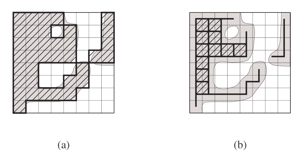
FIG. 1.: Two definitions of the Euler characteristic of a random field on a lattice. The excursion set $S_{u}$ (the shaded curved region in both figures) consists of all points where the field values are above the level $u$. (a) The diagonally adjacent pixels are considered to be connected, making one connected patch with two holes (shown in thick lines and hatching); the Euler characteristic is $1-2=-1$. (b) The diagonally adjacent pixels are not considered to be connected, which in effect reduces the original set $S_{u}$ to a smaller set shown in thick lines and hatching. The Euler characteristic is equal to $2$. The difference between the two definitions disappears with small enough lattice size.

The two definitions $\chi_{1}$ and $\chi_{2}$ on the square lattice are equally valid approximations of the Euler characteristic of the continuous excursion set, as will be any linear combination of the two. By inspection of Eqs. (50), (51) one finds that the simple average of $\chi_{1}$ and $\chi_{2}$,

$$\chi\left(S_{u}\right)=\frac{\chi_{1}\left(S_{u}\right)+\chi_{2}\left(S_{u}\right)}{2},$$ (52)

does not contain the sum over groups of four adjacent pixels and thus is the simplest to deal with. This definition counts one-half of all diagonally adjacent pairs of pixels. The averaging recipe has further advantages when analyzing the Gaussian case, suggesting that the definition (52) is the most suitable for square lattices.

Eqs. (48), (50)–(52) can be used to compute the Euler characteristic for a given map on a hexagonal and a square lattice, respectively. As in Eq. (33), the sums over groups of adjacent pixels can be transformed into the sums over neighbors of each pixel, arriving to expressions which are manifestly linear in the total number of pixels.

We now express the expectation value of the Euler characteristic through the distributions $P_{n}$. From Eq. (51) for the square lattice we obtain

$$\left\langle\chi_{2}\left(S_{u}\right)\right\rangle = \sum_{s\in S}\left\langle N_{u}\left(s\right)\right\rangle-\sum_{L\left[s_{1}\cap s_{2}\right]\neq 0}\left\langle N_{u}\left(s_{1}\right)N_{u}\left(s_{2}\right)\right\rangle$$ (54)

$$\ +\sum_{s_{1}\cap s_{2}\cap s_{3}\cap s_{4}\neq\emptyset}\left\langle N_{u}\left(s_{1}\right)N_{u}\left(s_{2}\right)N_{u}\left(s_{3}\right)N_{u}\left(s_{4}\right)\right\rangle.$$

The first term of Eq. (54) has already been calculated:

$$\sum_{s\in S}\left\langle N_{u}\left(s\right)\right\rangle=NP_{1}\left(u\right).$$ (55)

In the second term, we only need to count the pairs of squares separated by the distance $\Delta$. For each square there are four possible pairs, and we have to divide by $2$ to prevent double counting of pairs. Therefore, the second sum in Eq. (54) is

$$\sum_{L\left[s_{1}\cap s_{2}\right]\neq 0}\left\langle N_{u}\left(s_{1}\right)N_{u}\left(s_{2}\right)\right\rangle=2NP_{2}\left(u;\Delta\right).$$ (56)

Finally, the third sum in Eq. (54) is

$$\sum_{s_{1}\cap s_{2}\cap s_{3}\cap s_{4}\neq\emptyset}\left\langle N_{u}\left(s_{1}\right)N_{u}\left(s_{2}\right)N_{u}\left(s_{3}\right)N_{u}\left(s_{4}\right)\right\rangle=NP_{4}\left(u;\Delta\right),$$ (57)

where $P_{4}\left(u;\Delta\right)$ is the probability that $f\left(s\right)>u$ at four points $s_{1}$, $s_{2}$, $s_{3}$, $s_{4}$ situated at the vertices of a square with side $\Delta$. If we know the distributions $P_{i}$, $i=1,2,4$, for the random field $f$, then the average Euler characteristic $\chi$ per unit area from Eq. (54) is

$$\frac{\left\langle\chi_{2}\left(S_{u}\right)\right\rangle}{A\left(S\right)}=\frac{1}{\Delta^{2}}\left[P_{1}\left(u\right)-2P_{2}\left(u;\Delta\right)+P_{4}\left(u;\Delta\right)\right].$$ (58)

The other definition (50) of the Euler characteristic for the square lattice leads to the more complicated expression

$$\frac{\left\langle\chi_{1}\left(S_{u}\right)\right\rangle}{A\left(S\right)}=\frac{1}{\Delta^{2}}\left[P_{1}\left(u\right)-2P_{2}\left(u;\Delta\right)-2P_{2}\left(u;\Delta\sqrt{2}\right)+4P_{3}\left(u;\Delta,\Delta\sqrt{2}\right)-P_{4}\left(u;\Delta\right)\right],$$ (59)

where $P_{3}\left(u;\Delta,\Delta\sqrt{2}\right)$ is the probability for values at the vertices of a triangle with sides $\Delta$, $\Delta$, and $\Delta\sqrt{2}$ to be greater than $u$. Finally, the averaged definition of $\chi$, Eq. (52), is expressed as

$$\frac{\left\langle\chi\left(S_{u}\right)\right\rangle}{A\left(S\right)}=\frac{1}{\Delta^{2}}\left[P_{1}\left(u\right)-2P_{2}\left(u;\Delta\right)-P_{2}\left(u;\Delta\sqrt{2}\right)+2P_{3}\left(u;\Delta,\Delta\sqrt{2}\right)\right].$$ (60)

Analogous considerations for a regular hexagonal lattice yield the following expression for the average Euler characteristic per unit area:

$$\frac{\left\langle\chi\left(S_{u}\right)\right\rangle}{A\left(S\right)}=\frac{2}{\Delta^{2}\sqrt{3}}\left[P_{1}\left(u\right)-3P_{2}\left(u;\Delta\right)+2P_{3}\left(u;\Delta\right)\right],$$ (61)

where $P_{3}\left(u;\Delta\right)$ is the probability for the field values to be greater than $u$ at three points situated at vertices of an equilateral triangle with side $\Delta$.

The variance of $\chi$ can be calculated in essentially the same manner as the variance of $L$ in Eq. (47), with a similar if more cumbersome expression as the result. We omit that expression here and return to calculations of the variance of $\chi$ in Sec. IV.

E Boundary corrections

A typical experimentally obtained temperature map does not cover the full sky. Moreover, certain areas of the sky may be excluded from the map because of the presence of foreground sources such as our Galaxy or other reasons. The exclusions can be represented by taking the intersection of the full sky with an appropriate “window” domain $W$. If we denote by $S_{u}$ the excursion set of the temperature field if it were known throughout the full sky, then Eqs. (23), (34), (48)–(51) of the previous subsections will yield the values of the Minkowski functionals on the intersection of the full excursion set $S_{u}$ with the window $W$ normalized to the area of $W$, i.e. one would obtain $M_{i}\left(S_{u}\cap W\right)/A\left(W\right)$. Although these values can be regarded as samples of the “true” functionals $M_{i}\left(S_{u}\right)/A(S)$ normalized to the full sky area $A(S)$, the existence of the boundary of $W$ introduces systematic errors which should be removed before comparing the experimental values of $M_{i}\left(S_{u}\right)/A(S)$ with theoretical predictions. This is essentially what we mean by boundary corrections.

In practice, we shall not need to assume that $S_{u}$ is defined on a full sky $S$, but only that $S$ covers a sky region large enough to disregard any boundary effects. Since a full-sky map is defined on a sphere, in principle additional complications due to curvature arise in calculations of the Minkowski functionals; one indication of trouble is the fact that a sphere cannot be tiled with an arbitrarily fine-grained lattice of regular polygons. However, any curvature corrections should be negligible as long as the pixel dimensions are small compared to the curvature scale, and any lattice irregularities can be dealt with individually using the general expressions Eqs. (16) and (18). For simplicity, we limit the following considerations to a suitably large flat region of the sky covered by a regular lattice.

Some recipes for the boundary corrections have been proposed in the literature, in particular, for calculating the Euler characteristic (Coles 1988). One natural procedure (Mecke et al. 1994) is based on the kinematic property, Eq. (13). Let $K_{2}=W$ be a fixed-shape window domain and $K_{1}=S$ the underlying sky domain. By considering the measured $M_{i}(S_{u}\cap W)$ to be estimators for $\left\langle M_{i}(S_{u}\cap W)\right\rangle$, Eq. (13) can be inverted to obtain the boundary correction formulas

$$\frac{A\left(S_{u}\right)}{A(S)} = \frac{A\left(S_{u}\cap W\right)}{A(W)},$$ (63)

$$\frac{L\left(S_{u}\right)}{A(S)} = \frac{L\left(S_{u}\cap W\right)}{A(W)}-\frac{A\left(S_{u}\right)}{A(S)}\frac{L(W)}{A(W)},$$ (64)

$$\frac{\chi\left(S_{u}\right)}{A(S)} = \frac{\chi\left(S_{u}\cap W\right)}{A(W)}-\frac{A\left(S_{u}\right)}{A(S)}\frac{\chi(W)}{A(W)}-\frac{1}{2\pi}\frac{L\left(S_{u}\right)}{A(S)}\frac{L(W)}{A(W)}.$$ (65)

(note that we need to substitute $L\left(S_{u}\right)$ from Eq. (64) to Eq. (65)). These formulas hold for any shape of the window domain $W$. It is of course impossible to calculate the Minkowski functionals in a larger region than that in which the field is actually measured, but if the measured region accurately represents the properties of the field in the entire region, the above boundary correction formulas will be accurate. Unless the cosmological microwave signal exhibits strongly non-Gaussian features on the characteristic scales of the window domain (i.e. individual pixels from point sources or the galactic cut) this is likely to be an excellent assumption.

IV Minkowski functionals for Gaussian fields

In this section, we derive the expectation values of the Minkowski functionals for Gaussian fields defined on a lattice. First, we treat the area functional and compute its expectation value and variance. We then explore the feature of smoothness of random fields which is important for understanding the dependence of the Minkowski functionals on the pixel size. We derive the expectation value of the boundary length functional on arbitrary lattices and show explicitly its dependence on the lattice size and geometry. The expectation value of the Euler characteristic is then computed for the hexagonal lattice.

A Description of Gaussian fields

For a homogeneous Gaussian field $f$ with zero mean, the two-point correlation function

$$C\left(s_{1},s_{2}\right)=\left\langle f\left(s_{1}\right)f\left(s_{2}\right)\right\rangle\equiv C\left(r\right),\quad r\equiv\left|s_{1}-s_{2}\right|,$$ (66)

completely characterizes the field. Customarily, Gaussian random fields are specified by their power spectrum $S\left(k\right)$ which is the Fourier transform of the correlation function, expressed in two dimensions as

$$C\left(r\right)=\int_{0}^{\infty}kJ_{0}\left(kr\right)S\left(k\right)dk.$$ (67)

However, our present considerations are based on the physical space ($r$) rather than on the momentum space ($k$), so the correlation function $C\left(r\right)$ is more relevant in this context than the power spectrum.

For simplicity, we assume that the variance of the field (which is the same at all points) is $\left\langle f^{2}\right\rangle\equiv C\left(0\right)=1$. (This can always be achieved by normalizing the field, $f=\bar{f}\sigma$, if the original field had variance $\sigma^{2}$. To recover the original variables, one only needs to divide the function values $f$ by $\sigma$ and the correlation function $C$ by $\sigma^{2}$ in all formulas.) The correlation function of the normalized field will then satisfy $\left|C\left(r\right)\right|\leq 1$. Also, since correlations between distant points should be absent, the correlation function must satisfy $C\left(r=\infty\right)=0$.

Calculations of the Minkowski functionals require the distribution functions $P_{1}\left(u\right)$, $P_{2}\left(u;r\right)$, and so on, introduced in the previous section. These functions describe the probabilities of encountering field values smaller than the level $u$ simultaneously at some given points $s_{1}$, $s_{2}$, …, $s_{n}$ and can be expressed through the $n$-point probability densities $p_{n}\left(f_{1},...,f_{n}\right)$ for values $f_{i}\equiv f\left(s_{i}\right)$ at these points, cf. Eq. (22):

$$P_{n\,}\left(u\right)=\int_{u}^{\infty}df_{1}...\int_{u}^{\infty}df_{n}p_{n}\left(f_{1},...,f_{n}\right).$$ (68)

Since the field $f$ is Gaussian, all its $n$-point densities are finite-dimensional Gaussian distributions with probability densities of the form

$$p_{n}\left(f_{1},...,f_{n}\right)=\frac{1}{\left(2\pi\right)^{n/2}\sqrt{\det B}}\exp\left(-B^{ij}f_{i}f_{j}\right)$$ (69)

with suitable coefficients $B^{ij}$ forming a positive-definite matrix. As is well known, the matrix $B^{ij}$ is the inverse of the correlation matrix $C_{ij}\equiv\left\langle f\left(s_{i}\right)f\left(s_{j}\right)\right\rangle$. Since the field is homogeneous, the coefficients $C_{ij}$ are completely determined by the separations between points $s_{i}$ and $s_{j}$, i.e. $C_{ij}=C\left(\left|s_{i}-s_{j}\right|\right)$. Note that the presence of Gaussian pixel noise can be easily described at this stage. Imposition of noise with fixed standard deviation $\sigma^{2}$ on a Gaussian field with given $C\left(r\right)$ increases the value $C\left(0\right)$ by $\sigma^{2}$ while not changing $C\left(r\right)$ at any other point. (For a discrete map, the function $C\left(r\right)$ is only available on a discrete set of values $r=0$, $\Delta$, and so on.) We give the explicit form of $p_{2}\left(f_{1},f_{2}\right)$ in Appendix A, including the pixel noise correction.

B Area and its variance

We now consider the area functional of a Gaussian field. As follows from Eq. (24), the expectation value of the normalized area functional is equal to the value of the distribution function $P_{1}\left(u\right)$ defined in the preceding section. The one-point probability density for the values of the field is

$$p_{1}\left(f\right)=\frac{1}{\sqrt{2\pi}}\exp\left(-\frac{f^{2}}{2}\right),$$ (70)

and therefore the one-point distribution function is

$$P_{1}\left(u\right)=\int_{u}^{\infty}p_{1}\left(f\right)df=\frac{1}{2}\left(1-\mathop{\rm erf}\frac{u}{\sqrt{2}}\right).$$ (71)

This is the expectation value of the area of the excursion set $S_{u}$ per unit area of the region.

The variance of the area functional is approximately given by Eq. (30),

$$\text{var}\left[\frac{A\left(S_{u}\right)}{A\left(S\right)}\right]=\frac{1}{A\left(S\right)}\int_{0}^{r_{0}}2\pi rdr\left\{P_{2}\left(u;r\right)-\left[P_{1}\left(u\right)\right]^{2}\right\}.$$ (72)

Since the integrand is assumed to vanish at $r>r_{0}$, the upper limit in Eq. (72) can be extended to infinity. As shown in Eq. (B15) of Appendix B, the two-point distribution function $P_{2}\left(u;r\right)$ can be expressed through the correlation function $C\left(r\right)$ as

$$P_{2}\left(u;r\right)=\left[P_{1}\left(u\right)\right]^{2}+\int_{0}^{C\left(r\right)}\frac{dC}{2\pi\sqrt{1-C^{2}}}\exp\left(-\frac{u^{2}}{1+C}\right).$$ (73)

Then we can transform Eq. (72) into

$$\text{var}\left[\frac{A\left(S_{u}\right)}{A\left(S\right)}\right] = \frac{1}{A\left(S\right)}\int_{0}^{\infty}2\pi rdr\int_{0}^{C\left(r\right)}\frac{dC}{2\pi\sqrt{1-C^{2}}}\exp\left(-\frac{u^{2}}{1+C}\right)$$ (74)

$$= \frac{1}{A\left(S\right)}\int_{0}^{1}\frac{r^{2}\left(C\right)dC}{2\sqrt{1-C^{2}}}\exp\left(-\frac{u^{2}}{1+C}\right),$$ (75)

where we have changed the order of integration and used the inverse $r\left(C\right)$ of the correlation function $C\left(r\right)$. Thus, Eq. (75) allows one to calculate (at least numerically) the variance of the area functional at a given level $u$ for any given correlation function $C\left(r\right)$. The maximum of the variance (at $u=0$), as can be seen from Eq. (75) and as we have checked for some sample functions $C\left(r\right)$, is proportional to $r_{0}^{2}/A\left(S\right)$, where $r_{0}$ is the typical distance at which correlations vanish, in agreement with the qualitative estimate (31).

We can also obtain the asymptotic form of the variance in the limit of large levels $\left|u\right|$, for which the integral in Eq. (75) is dominated by the neighborhood of $C=1$ (small distances). We assume a Taylor expansion of the correlation function $C\left(r\right)$ at small distances,

$$C\left(\Delta\right)=1-C_{1}\left(\frac{\Delta}{r_{1}}\right)^{p}+{\cal O}\left(\Delta^{p+1}\right),$$ (76)

where $C_{1}$, $r_{1}$ and $p<2$ are some constants. Then by expanding the integrand in $\left(1-C\right)$ we obtain the leading term

$$\text{var}\left[\frac{A\left(S_{u}\right)}{A\left(S\right)}\right]\simeq{\pi r_{1}^{2}\over A\left(S\right)C_{1}^{2/p}}\,\Gamma\left({4+p}\over{2p}\right)\left({u^{2}\over 2}\right)^{-(4+p)/2p}\exp\left(-{u^{2}\over 2}\right).$$ (77)

The square root of the variance (77) is proportional to $\exp\left(-u^{2}/4\right)$ and at large enough $u$ becomes large relative to the “signal” itself which, as follows from Eq. (71), is proportional to $\exp\left(-u^{2}/2\right)$. This is to be expected for all Minkowski functionals, since the signal at large $u$ comes from very few map pixels. Thus, we can only use features of the Minkowski functional profiles at levels $u$ within a few standard deviations from the average.

C Smooth random fields

A random field is continuous if the values at nearby points are highly correlated. For a continuous field, the limit of the correlation function at vanishing distance must be

$$\lim_{\Delta\rightarrow 0}C\left(\Delta\right)=C\left(0\right)\equiv 1,$$ (78)

i.e. the correlation function must be continuous at $\Delta=0$. We shall call a continuous random field smooth (with a somewhat relaxed rigor) if its spatial derivatives are finite, i.e. have finite variances. To see what this means mathematically, consider a homogeneous one-dimensional random field $f\left(x\right)$ with a given correlation function $C\left(r\right)$. The variance of a finite-differenced derivative $\left(f\left(x+\Delta\right)-f\left(x\right)\right)/\Delta$ is

$$\frac{1}{\Delta^{2}}\left\langle\left[f\left(x+\Delta\right)-f\left(x\right)\right]^{2}\right\rangle=2\frac{1-C\left(\Delta\right)}{\Delta^{2}}.$$ (79)

We call the field $f$ smooth if Eq. (79) has a finite limit at $\Delta\rightarrow 0$. This happens for instance if the correlation function is regular at $\Delta=0$ with vanishing first derivative,

$$C\left(\Delta\right)=1-{1\over 2}C^{\prime\prime}(0)\Delta^{2}+{\cal O}\left(\Delta^{3}\right).$$ (80)

In general, if the asymptotic form of the correlation function for small $\Delta$ is a power law, Eq. (76), then if $p<2$ the field is not smooth. Physically, a random field is smooth if its small-wavelength modes are suppressed strongly enough so that the field values at nearby points are highly correlated. One can show, for instance, that if the small-wavelength modes in the power spectrum of a Gaussian random field (cf. Eq. (67)) are exponentially suppressed, as in the power spectrum

$$S\left(k\right)\propto k^{n}\exp\left(-ak\right)\text{ as }k\rightarrow+\infty,$$ (81)

then the correlation function $C\left(r\right)$ satisfies Eq. (80) and the field is smooth.

Although the CMB temperature is expected to be smooth because of Silk damping of CMB fluctuations on scales below a few arcminutes, the behavior of the correlation function on larger scales, particularly the pixel size of a given experimental map, may differ from Eq. (80). This could make the CMB temperature field effectively non-smooth on the pixelization scale. As we show below, excursion sets of non-smooth fields have a fractal shape manifested by the scaling of the $L$ and $\chi$ functionals with the pixel size. In our subsequent analysis, we shall not assume that the correlation function possesses an expansion of type (80) on the relevant pixel scales.

D Boundary length for a Gaussian field

The average boundary length $L\left(S_{u}\right)$ per unit area can be found using Eq. (37). We need to know the probability distribution $P_{2}\left(u;\Delta\right)$ for values $f_{1,2}$ at two points $s_{1,2}$ separated by the pixel size $\Delta$. Substituting Eq. (B12) from Appendix B into Eq. (37), we obtain

$$\frac{\left\langle L\left(S_{u}\right)\right\rangle}{A\left(S\right)}=\frac{2}{\pi\Delta}\int_{C\left(\Delta\right)}^{1}\frac{dC}{\sqrt{1-C^{2}}}\exp\left(-\frac{u^{2}}{1+C}\right).$$ (82)

For small enough $\Delta$ the values of the correlation function $C\left(\Delta\right)$ are close to $1$, so we can expand the above integral in powers of the small parameter $\epsilon\equiv 1-C\left(\Delta\right)$ and obtain

$$\frac{\left\langle L\left(S_{u}\right)\right\rangle}{A\left(S\right)} = \frac{2\sqrt{2\epsilon}}{\pi\Delta}\exp\left(-\frac{u^{2}}{2}\right)\left[1+\frac{1-u^{2}}{12}\epsilon+\frac{3-6u^{2}+u^{4}}{160}\epsilon^{2}\right.$$ (84)

$$\qquad+\frac{15-45u^{2}+15u^{4}-u^{6}}{2688}\epsilon^{3}+\left.\frac{105-420u^{2}+210u^{4}-28u^{6}+u^{8}}{55296}\epsilon^{4}+{\cal O}\left(\epsilon^{5}\right)\right].$$

This expansion holds, as does Eq. (37), for all regular lattices; the expansion parameter $\epsilon$ is typically a power of the lattice step $\Delta$. We note that the dependence on $\Delta$ appears already in the leading term. If the field is smooth and its correlation function is described by Eq. (80), then it is easily seen that the leading term of Eq. (84) is independent of $\Delta$ in the limit of small $\Delta$. However, for non-smooth fields the dependence on $\Delta$ does not go away and may lead to formal divergence of $L$ at small $\Delta$. For instance, if the correlation function satisfies Eq. (76) in some range of $\Delta$, then the leading term scales with $\Delta$ as $\Delta^{p/2-1}$. The scaling property of the leading term can be interpreted as a manifestation of fractal geometry of the contour lines with fractal dimension $2-p/2>1$.

It is interesting to compare the series (84) and the result for the length of level contours of a continuous smooth Gaussian field in two dimensions [Adler 1981],

$$\frac{\left\langle L\left(S_{u}\right)\right\rangle}{A\left(S\right)}=\frac{\sqrt{-C^{\prime\prime}\left(0\right)}}{2}\exp\left(-\frac{u^{2}}{2}\right).$$ (85)

With the correlation function (80), the leading term of Eq. (84) reproduces the continuous limit (85) up to the factor $4/\pi$. This discrepancy is due to the fact that the length of a discrete approximation of a line by a fixed regular lattice differs from the length of the line by a geometric factor. This factor is easiest to derive for the square lattice, where a curved line is approximated by horizontal and vertical straight line segments. For lattice steps $\Delta$ much smaller than the typical radius of curvature, the curve is locally well-approximated by a straight line. If a straight line segment of length $L$ makes an angle $\alpha$ with the lattice (see Fig. 2a), then the length of its lattice approximation is $\tilde{L}=L\left(\cos\alpha+\sin\alpha\right)$. Averaging this over all angles $\alpha$ (it suffices to consider $0<\alpha<\pi/2$), we obtain

$$\left\langle\tilde{L}\right\rangle_{\alpha}=\frac{2}{\pi}\int_{0}^{\pi/2}L\left(\cos\alpha+\sin\alpha\right)d\alpha=\frac{4}{\pi}L.$$ (86)

This means that the lattice approximation of the length of a curve with isotropically distributed tangent angle is wrong by a factor of $4/\pi$ on the average. By a similar argument it can be shown that any tiling by identical regular polygons gives rise to the same factor $4/\pi$. (In the case of non-regular tilings, the correction factor will generally differ from $4/\pi$, and also the higher terms of the series (84) will be different.)

A more intuitive way to obtain this correction factor $4/\pi$ is to consider a square with an inscribed circle. The length of the lattice approximation to the circle is equal to the perimeter of the square (see Fig. 2b). The ratio of the circumferences is $4/\pi$. The circle effectively averages over all orientations of the line, therefore the result also holds on the average for curved lines with isotropically distributed tangent angles.

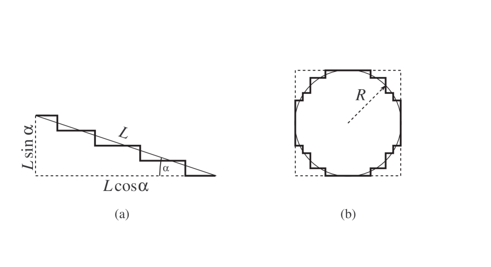
FIG. 2.: Geometric correction factor for curves on a lattice. (a) Approximation of a straight line segment $L$ making an angle $\alpha$ with the lattice has length $L\left(\cos\alpha+\sin\alpha\right)$. Averaging this over the angles $\alpha$ yields $4L/\pi$. (b) The circumference of a circle, $2\pi R$, is approximated by a rectangular lattice. The result, even for an arbitrarily fine lattice, is $8R$, which is off by the same factor $4/\pi$.

Apart from the geometric correction factor, a comparison of the series (84) with the continuous limit (85) shows that higher terms of the series contain polynomials in $u$ which distort the Gaussian profile. The resulting small deviation from Eq. (85) is a direct consequence of pixelization. While Eq. (84) holds for any regular lattice, in particular for square and hexagonal lattices, in asymmetric lattices the coefficients of the series for $L$ depend on the pixel geometry.

Application of the general formula of Eq. (47) for the variance to the Gaussian case requires calculation of the distribution $P_{4}\left(u;\Delta,r\right)$ for the two pairs of closest neighbor points separated by the distance $r$. In Appendix B, an expansion of the distribution $P_{4}\left(u;\Delta,r\right)$ in powers of $\epsilon\equiv 1-C\left(\Delta\right)$ is found. We retain only the leading term of this expansion, because the error of the approximation in Eq. (47) is typically worse than the contribution $O\left(\epsilon\right)$ of the higher terms of the expansion. The resulting expression for the variance of $L$ is

$$\text{var}\left[\frac{L\left(S_{u}\right)}{A\left(S\right)}\right]\approx\left(\frac{2}{\pi\Delta}\right)^{2}\frac{2\epsilon}{\pi r_{\max}^{2}}\int_{0}^{r_{\max}}\left[\left(1-C(r)^{2}\right)^{-1/2}\exp\left(-{u^{2}\over 1+C(r)}\right)-\exp\left(-u^{2}\right)\right]2\pi rdr.$$ (87)

As in the previous section, one can transform this integral to the variable $C\left(r\right)$ and show that the asymptotic form of the variance (87) at large $\left|u\right|$ is proportional to $\exp\left(-u^{2}/2\right)$.

E The Euler characteristic

Finally we consider the Euler characteristic of the excursion set per unit area. We first consider the simpler case of a hexagonal lattice for which the Euler characteristic is given by Eq. (61). Using Eq. (B31) from Appendix B and expanding it in powers of the small parameter $\epsilon\equiv 1-C\left(\Delta\right)$, we obtain the series

$$\frac{\left\langle\chi\left(S_{u}\right)\right\rangle}{A\left(S\right)} = \frac{2u\exp(-u^{2}/2)}{\left(2\pi\right)^{3/2}\Delta^{2}}\epsilon\left[1+5\frac{3-u^{2}}{36}\epsilon+7\frac{15-10u^{2}+u^{4}}{540}\epsilon^{2}\right.$$ (89)

$$+83\frac{105-105u^{2}+21u^{4}-u^{6}}{90720}\epsilon^{3}\left.+319\frac{945-1260u^{2}+378u^{4}-36u^{6}+u^{8}}{6123600}\epsilon^{4}+{\cal O}\left(\epsilon^{5}\right)\right].$$

The leading term of the series (89) coincides with the formula of Adler (1981) for the average Euler characteristic of excursion sets of a smooth Gaussian field,

$$\frac{\left\langle\chi\right\rangle}{A\left(S\right)}={|C^{\prime\prime}(0)|\over(2\pi)^{3/2}}\,u\exp\left(-{u^{2}\over 2}\right)$$ (90)

The case of a square lattice is more complicated. We can use the methods of Appendix B to obtain a series expansion of Eqs. (58)–(60). However, since the point configurations for the required distributions $P_{3}$ and $P_{4}$ contain neighbors separated by distances $\Delta$ and $\Delta\sqrt{2}$, there are now two small parameters, namely $\epsilon\equiv 1-C\left(\Delta\right)$ and $b\epsilon\equiv 1-C\left(\Delta\sqrt{2}\right)$, where we have introduced the parameter $b$ which is of order $1$ and which characterizes the behavior of the correlation function $C\left(r\right)$ at smallest distances available on the lattice,

$$b\equiv\frac{1-C\left(\Delta\sqrt{2}\right)}{1-C\left(\Delta\right)}.$$ (91)

By definition, $b>0$; moreover, one can derive the condition $b<2$ from the requirement of normalizability of the four-point distribution $p_{4}$ for the corners of a closest neighbor square (cf. Appendix A, Eq. (A3) with the correlation matrix of Eq. (A6)). A smooth Gaussian field satisfying Eq. (80) is described by $b\approx 2$, and the deviation of $b$ from $2$ is of order $1-C\left(\Delta\right)$. From a given experimental map, the parameter $b$ can be estimated in linear time. If the value of $b$ is significantly smaller than $2$, namely if $2-b\gg 1-C\left(\Delta\right)$, we conclude that the underlying field is not smooth on scales $\Delta$.

After computing the expansions of Eqs. (58)–(60) in $\epsilon$ (while keeping the parameter $b$ constant), one finds in each case an expression similar to Eq. (89), except that both the leading term and the coefficients of the polynomials in $u$ in the higher terms depend on $b$. However, the most significant difference is that the leading term of the expansion of Eqs. (58) and (59) is not of order $\epsilon$ but of order $\sqrt{\epsilon}$, and also the expansion parameter of the series is $\sqrt{\epsilon}$ instead of $\epsilon$. The first two terms of the expansion of Eq. (59) are

$$\frac{\left\langle\chi_{2}\left(S_{u}\right)\right\rangle}{A\left(S\right)}={1\over\sqrt{2}\pi^{2}\Delta^{2}}\left(2\arccos{b\over 4-b}-\sqrt{b}\arccos{3b-4\over 4-b}\right)\exp\left(-{u^{2}\over 2}\right)\sqrt{\epsilon}+{\sqrt{b(4-b)}\over(2\pi)^{3/2}\Delta^{2}}\,u\exp\left(-{u^{2}\over 2}\right)\epsilon+{\cal O}\left(\epsilon^{3/2}\right).$$ (92)

At $b=2-O\left(\epsilon\right)$, which corresponds to a smooth field, the first term as well as all terms with non-integer powers of $\epsilon$ vanish, and the series (92) becomes again a series in $\epsilon$. For non-smooth fields, however, Eq. (92) does not correspond to its continuous limit Eq. (90).

A similar result is obtained for $\chi_{1}$, Eq. (58). The situation is however different with the Euler characteristic defined by Eq. (60): all terms with non-integer powers of $\epsilon$ cancel, and the result is

$$\frac{\left\langle\chi\left(S_{u}\right)\right\rangle}{A\left(S\right)} = {\sqrt{b(4-b)}\over(2\pi)^{3/2}\Delta^{2}}\,u\exp\left(-{u^{2}\over 2}\right)\epsilon\left[1+\frac{\left(3-u^{2}\right)\left(4+2b-b^{2}\right)}{12\left(4-b\right)}\epsilon\right.$$ (95)

$$\qquad+\frac{\left(b^{4}-6b^{3}+6b^{2}+2b+18\right)\left(u^{4}-10u^{2}+15\right)}{180\left(4-b\right)^{2}}\epsilon^{2}$$

$$\qquad\left.+\,\frac{\left(b^{6}-10b^{5}+30b^{4}-20b^{3}-12b^{2}+8b-80\right)\left(u^{6}-21u^{4}+105u^{2}-105\right)}{3360\left(4-b\right)^{3}}\epsilon^{3}\right]+{\cal O}\left(\epsilon^{5}\right)$$

The series (95) is reduced to Eq. (89) at $b=1$. The leading term of this series is, up to a constant, the same as the continuous limit Eq. (90); the correspondence is exact at $b=2$. For this reason, we suggest that the “averaged” definition of $\chi$, Eq. (60), be used for square lattice calculations. As in the previous section, we note the scaling properties of Eqs. (89)–(95) with $\Delta$ and interpret them as a manifestation of the fractal structure of the excursion set. For smooth fields, the dependence on $\Delta$ cancels out, while for non-smooth fields it may lead to a divergence of $\chi$ at small $\Delta$.

The variance of $\chi$ can be estimated similarly to the variance of the boundary length $L$, except that the expressions of Eqs. (60), (61) for $\chi$ contain $3$-point distributions $P_{3}$ and therefore its variance requires calculation of the $6$-point distribution $P_{6}$. This calculation can also be performed by methods presented in Appendix B and, as in the case of the variance of $L$, only the leading term of the resulting expansion suffices up to the precision of approximation. We give the result for the variance of the Euler characteristic only in the simplest case on hexagonal lattice:

$$\text{var}\left[\frac{\chi\left(S_{u}\right)}{A\left(S\right)}\right]\simeq\frac{\epsilon^{2}}{\Delta^{4}\pi^{3}r_{\max}^{2}}\int_{0}^{r_{\max}}\left[\frac{u^{2}\left(1-C\right)+C\left(1+C\right)}{\sqrt{1-C^{2}}\left(1-C\right)\left(1+C\right)^{2}}\exp\left(-\frac{u^{2}}{1+C}\right)-u^{2}\exp\left(-u^{2}\right)\right]rdr,$$ (96)

where we imply $C\equiv C\left(r\right)$. The properties of the variance of $\chi$ are similar to those of the variances of the other two Minkowski functionals, as has been discussed above.

V SUMMARY AND DISCUSSION

In this paper, we have proposed the Minkowski functionals – area, boundary length, and Euler characteristic – of excursion sets as a probe of a map’s Gaussianity. They are all linear functions of the number of map pixels, and thus are easy to compute from a map. Gaussian pixel noise is straightforward to include, and irregular map boundaries, arising from partial sky coverage or cuts of the data, can be accounted for in a natural manner. Finally, for Gaussian distributions the functionals can be calculated exactly and their variances estimated given the correlation function of the distribution, making a test of Gaussianity straightforward and eliminating the need for Monte Carlo simulations.

We have presented a complete formulation of Minkowski functionals on a two-dimensional pixelized map, including explicit boundary corrections and pixel-size dependences. We propose an alternative definition of the Euler characteristic for pixelized maps which possesses nice calculational properties compared with previously used definitions. In addition, we provide explicit forms of the functionals and their variances for the case of Gaussian distributions, including pixelization corrections.

Minkowski functionals are simplest to calculate for maps with hexagonal pixelation schemes, because no more than three pixels can ever adjoin a single point and all adjoining pixels are the same distance apart. This property also makes estimation of the Euler functional more straightforward and allows easier estimation of the variances of Gaussian map functionals. Hexagonal pixelizations also have other nice properties like optimal smoothness and regularity (Tegmark 1996). Analysis of maps with square pixels will be a bit more technically involved, but not fundamentally different. Actual full-sky maps will always have irregular points in the pixelization lattice (since the sphere cannot be tiled by identical polygons) which will need to be handled on an individual basis. No conceptual difficulties arise in extending the Minkowski functionals to a sphere as long as the pixelization scale is small compared to the curvature scale, which will always be the case for maps of moderately high resolution.

It is impossible to make a general statement about how well these functionals will distinguish non-Gaussianity in a map because the variety of non-Gaussianity is endless. Since Minkowski functionals are ensemble or map averages, it is likely they will be best at picking out non-Gaussian distributions which are spread over an entire map, as opposed to isolated, sharp features which will be lost in the averaging. Even if the primordial perturbations are Gaussian-distributed (as expected in inflationary models), potentially interesting non-Gaussianity might arise from weak gravitational lensing (Bernardeau 1996) or from Sunyaev-Zeldovich distortions. For a specific kind of non-Gaussian contribution, simulations of the resulting sky will be required to determine the utility of Minkowski functional analysis.

Any test of primordial non-Gaussianity in CMB maps is likely to be challenging with real data. Just as noise correlations can mimic CMB power (Dodelson and Kosowsky, 1995), any noise correlation will create non-Gaussianity in a map (Kogut et al. 1994). A meaningful Gaussianity test requires detailed understanding of an experiment’s noise properties. The best bet for Gaussianity tests are those experiments with simple noise properties; the MAP satellite design, for example, was driven largely by the desire for very simple noise properties. Other unavoidable noise correlations are induced by projecting out foreground contamination, but these correlations can likely be understood in detail through modelling and simulations. Conversely, for experiments with complicated noise properties, Minkowski functional analysis may aid in characterizing the noise as long as the underlying fluctuations are close to Gaussian.

Gaussian-distributed initial fluctuations are a decisive prediction of inflationary models. Upcoming CMB data sets in the form of high-resolution maps will allow meaningful tests of this prediction. The theoretical framework presented in this paper refines and extends the current menu of Gaussianity tests, and we anticipate that Minkowski functionals will be a basic component of future microwave background map analysis.

A Gaussian probability densities in several variables

We first consider the simplest case of the Gaussian two-point probability density $p_{2}\left(x,y;\Delta\right)$ for field values $x$, $y$ at points $s_{1,2}$ separated by the distance $\Delta$. For a normalized Gaussian field, the correlations are

$$\left\langle x^{2}\right\rangle = \left\langle y^{2}\right\rangle=1,$$

$$\left\langle xy\right\rangle = C\left(\Delta\right).$$

We can easily diagonalize the correlation matrix if we notice that

$$\left\langle\left(x+y\right)\left(x-y\right)\right\rangle = 0,$$

$$\left\langle\left(x\pm y\right)^{2}\right\rangle = 2\left(1\pm C\left(\Delta\right)\right),$$

which means that $\left(x+y\right)$ and $\left(x-y\right)$ are independent Gaussian variables with known variances. One can then write the joint distribution for $\left(x\pm y\right)$ as a product of two Gaussians,

$$p_{2}\left(x,y;\Delta\right)dxdy=\frac{dxdy}{2\pi\sqrt{1-C\left(\Delta\right)^{2}}}\exp\left[-\frac{1}{4}\left(\frac{\left(x+y\right)^{2}}{1+C\left(\Delta\right)}+\frac{\left(x-y\right)^{2}}{1-C\left(\Delta\right)}\right)\right].$$ (A1)

More generally, a multivariate Gaussian distribution in $n$ variables $x_{1}$, …, $x_{n}$ is completely specified by a symmetric correlation matrix $C_{ij}\equiv\left\langle x_{i}x_{j}\right\rangle$, and the joint probability density is expressed through the inverse matrix $C^{-1}$ by

$$p_{n}\left({\bf x};C_{ij}\right)d^{n}{\bf x}=\frac{d^{n}{\bf x}}{\left(2\pi\right)^{n/2}\sqrt{\det C_{ij}}}\exp\left[-\frac{1}{2}\sum_{i,j=1}^{n}C_{ij}^{-1}x_{i}x_{j}\right].$$ (A2)

If the matrix $C_{ij}$ is explicitly diagonalized and its eigenvalues $\lambda_{i}$ and the corresponding orthonormal eigenvectors $E_{i}^{j}$ are known, then the probability density $p_{n}\left({\bf x};C_{ij}\right)$ can be written as a product of Gaussians similar to Eq. (A1),

$$p_{n}\left({\bf x};C_{ij}\right)=\frac{1}{\left(2\pi\right)^{n/2}\sqrt{\det C_{ij}}}\exp\left[-\frac{1}{2}\sum_{i=1}^{n}\frac{\left(\sum_{j=1}^{n}E_{i}^{j}x_{j}\right)^{2}}{\lambda_{i}}\right].$$ (A3)

However, this explicit form of the distribution density will not be as useful as its representation as a Fourier transform of its generating function $\tilde{p}_{n}\left({\bf k};C_{ij}\right)$,

$$p_{n}\left({\bf x};C_{ij}\right)\equiv\int\frac{d^{n}{\bf k}}{\left(2\pi\right)^{n}}\tilde{p}_{n}\left({\bf k};C_{ij}\right)=\int\frac{d^{n}{\bf k}}{\left(2\pi\right)^{n}}\exp\left[i{\bf kx-}\frac{1}{2}\sum_{i,j=1}^{n}C_{ij}k_{i}k_{j}\right].$$ (A4)

This form of the probability density will be used in Appendix B for calculations of the probability integrals $P_{n}$ defined by Eq. (22).

The distributions for values of a homogeneous and isotropic Gaussian field at the vertices of an equilateral triangle or a square are found as special cases of the multivariate Gaussian distribution. The three-point distribution $p_{3}\left(x,y,z;C\right)$ is characterized by a single parameter, the correlation $C\equiv C_{12}=\left\langle xy\right\rangle=\left\langle yz\right\rangle=\left\langle zx\right\rangle$ between any two different points, while $C_{ii}\equiv 1$. The correlation matrix $C_{ij}$ is

$$C_{ij}=\left(\begin{array}[]{ccc}1&C&C\\ C&1&C\\ C&C&1\end{array}\right).$$ (A5)

Similarly, one obtains the four-point distribution $p_{4}\left(w,x,y,z\right)$ for values at the vertices of a square. This time the distribution has two free parameters, namely the correlations between the adjacent points $C_{12}\equiv C$ and between the diagonally opposing points $C_{23}\equiv D$. The correlation matrix $C_{ij}$ in that case is

$$C_{ij}=\left(\begin{array}[]{cccc}1&C&C&D\\ C&1&D&C\\ C&D&1&C\\ D&C&C&1\end{array}\right).$$ (A6)

The explicit forms of the distributions $p_{3}\left(x,y,z;C\right)$ and $p_{4}\left(w,x,y,z;C,D\right)$ can be obtained using Eq. (A3), but we omit them as they will not be useful for our calculations.

Finally we briefly describe how a known level of Gaussian pixel noise present in experimental maps can be represented in this formalism. If we assume that Eq. (A3) describes the $n$-point distribution obtained from a noiseless map, then pixel noise with a fixed variance $\sigma^{2}$ (in units of the field variance) will simply increase the diagonal elements of the matrix $C_{ij}$ by $\sigma^{2}$, while not changing any other correlations. Thus pixel noise can be straightforwardly incorporated by making the replacements $C_{ij}\rightarrow C_{ij}/(1+\sigma^{2})$ for $i\neq j$ in the correlation matrix.

B The Gaussian probability integrals

In this appendix we give some derivations for the distributions $P_{n}\left(u\right)$ which define the probability for the values of a Gaussian random field at $n$ given points to be above the threshold value $u$. Generally, these distributions, as defined by Eq. (68), involve multiple integrals of Gaussians of the type (A2) and cannot be exactly evaluated. However, if the correlation between the point values is high ($C_{ij}\approx 1$), as is the case for neighboring points of a fine lattice, one can develop series expansions of $P_{n}\left(u;C_{ij}\right)$ in powers of $\left(1-C_{ij}\right)$. We follow the calculations presented in Hamilton et al. (1986), where a method for computing the series expansions for the distributions $P_{2}$, $P_{3}$, and $P_{4}$ was presented, the expansion parameter being the lattice step $\Delta$. As we have seen in Sec. III, knowledge of these three distributions suffices to find the three Minkowski functionals on the plane. However, we do not assume an expansion of type (80) for the correlation function and keep $\left(1-C_{ij}\right)$ as expansion parameters instead of the lattice step $\Delta$, so that our results are applicable not only to smooth Gaussian fields. For completeness, we explain the method of calculation in some detail; this will also enable us to clarify the limitations of this method when applied to non-Gaussian distributions.

We start with the Fourier representation of a Gaussian two-point symmetric probability density,

$$p_{2}\left({\bf x};C\right) = \int\frac{d^{2}{\bf k}}{\left(2\pi\right)^{2}}\exp\left[i{\bf kx-}\frac{1}{2}\left(k_{1}^{2}+k_{2}^{2}\right)-Ck_{1}k_{2}\right]$$ (B1)

$$\equiv \int\frac{d^{2}{\bf k}}{\left(2\pi\right)^{2}}e^{i{\bf kx}}\tilde{p}_{2}\left({\bf k};C\right).$$ (B2)

The distribution (B2) is symmetric with respect to an interchange of $x_{1,2}$ and is characterized by the mean value $\left\langle x_{i}\right\rangle=0$, variance $\left\langle x_{i}^{2}\right\rangle=1$, and correlation $\left\langle x_{1}x_{2}\right\rangle=C$ with $\left|C\right|\leq 1$. The probability integral $P_{2}\left(u;C\right)$ is defined by

$$P_{2}\left(u;C\right)\equiv\int_{u}^{\infty}dx\int_{u}^{\infty}dy\,p_{2}\left({\bf x};C\right).$$ (B3)

This coincides with the distribution $P_{2}\left(u;C\left(\Delta\right)\right)$ defined by Eq. (21).

One then takes the partial derivative of $P_{2}\left(u;C\right)$ with respect to $C$. Since

$$\frac{\partial}{\partial C}\tilde{p}_{2}\left({\bf k};C\right)=-k_{1}k_{2}\tilde{p}_{2}\left({\bf k};C\right),$$ (B4)

it follows that

$$\frac{\partial}{\partial C}P_{2}\left(u;C\right)=-\int_{u}^{\infty}dx\int_{u}^{\infty}dy\int\frac{d^{2}{\bf k}}{\left(2\pi\right)^{2}}k_{1}k_{2}e^{i{\bf kx}}\tilde{p}_{2}\left({\bf k};C\right).$$ (B5)

To change the order of integration in Eq. (B5), it is necessary to replace the infinite upper limits in the integrations over $x$ and $y$ by a finite quantity $M$ and take the limit of $M\rightarrow\infty$ afterwards. The integrations over $x$ and $y$ yield

$$\int_{u}^{M}dx\int_{u}^{M}dye^{i{\bf kx}}=\frac{e^{ik_{1}M}-e^{ik_{1}u}}{ik_{1}}\frac{e^{ik_{2}M}-e^{ik_{2}u}}{ik_{2}}.$$ (B6)

The factor $k_{1}k_{2}$ in Eq. (B5) cancels. The distribution density $p_{2}\left({\bf x};C\right)$ decays at spatial infinity, so

$$\frac{\partial}{\partial C}P_{2}\left(u;C\right)=\lim_{M\rightarrow\infty}\left[p_{2}\left(u,u;C\right)-2p_{2}\left(u,M;C\right)+p_{2}\left(M,M;C\right)\right]=p_{2}\left(u,u;C\right).$$ (B7)

By means of this relation, the double probability integral in Eq. (B3) is reduced to a single integral

$$P_{2}\left(u;C\right)=P_{2}\left(u;1\right)-\int_{C}^{1}\,p_{2}\left(u,u;C\right)dC.$$ (B8)

Here we choose the boundary condition at $C=1$ which corresponds to the limit of two coincident points, where the two-point distribution degenerates into a one-point Gaussian,

$$p_{2}\left(x,y;1\right)=\frac{\delta\left(x-y\right)}{\sqrt{2\pi}}\exp\left(-\frac{x^{2}}{2}\right),$$ (B9)

so it easily follows that

$$P_{2}\left(u;1\right)\equiv P_{1}\left(u\right)=\frac{1}{2}\left(1-\mathop{\rm erf}\left[\frac{u}{\sqrt{2}}\right]\right).$$ (B10)

Now substituting into Eq. (B8) the explicit form of the distribution from Eq. (A1),

$$p_{2}\left(u,u;C\right)=\frac{1}{2\pi\sqrt{1-C^{2}}}\exp\left[-\frac{u^{2}}{1+C}\right],$$ (B11)

gives

$$P_{2}\left(u;C\right)=P_{1}\left(u\right)-\int_{C}^{1}\frac{dC}{2\pi\sqrt{1-C^{2}}}\exp\left[-\frac{u^{2}}{1+C}\right].$$ (B12)

Although the resulting integral cannot be evaluated analytically, it is easily expanded in powers of $\left(1-C\right)\equiv\epsilon$,

$$\int_{1-\epsilon}^{1}\frac{dx}{\sqrt{1-x^{2}}}\exp\left[-\frac{u^{2}}{1+x}\right]=\sqrt{2\epsilon} \,\exp\left(-\frac{u^{2}}{2}\right)\left[1+\frac{1-u^{2}}{12}\epsilon+\frac{3-6u^{2}+u^{4}}{160}\epsilon^{2}\right.$$ (B13)

$$+\frac{15-45u^{2}+15u^{4}-u^{6}}{2688}\epsilon^{3}+ \left.\frac{105-420u^{2}+210u^{4}-28u^{6}+u^{8}}{55296}\epsilon^{4}+O\left(\epsilon^{5}\right)\right].$$ (B14)

Another possible choice of the boundary condition is $C=0$. The two-point distribution $p_{2}$ degenerates into a product of two one-point distributions $p_{1}$, which leads to the following result,

$$P_{2}\left(u;C\right)=\left[P_{1}\left(u\right)\right]^{2}+\int_{0}^{1}\frac{dC}{2\pi\sqrt{1-C^{2}}}\exp\left[-\frac{u^{2}}{1+C}\right].$$ (B15)

As has been already noted by Hamilton et al. (1986), an extension of this technique to non-Gaussian distributions is problematic. Namely, one might consider the Fourier representation of a non-Gaussian two-point distribution

$$p_{2}\left({\bf x};C,D,...\right)=\int\frac{d^{2}{\bf k}}{\left(2\pi\right)^{2}}\exp\left[i{\bf kx-}\frac{1}{2}\left(k_{1}^{2}+k_{2}^{2}\right)-Ck_{1}k_{2}-\sum D_{ijl}k_{i}k_{j}k_{l}+...\right],$$ (B16)

where the coefficients $D_{ijl}$ and the (omitted) higher-order terms of the series in ${\bf k}$ represent deviations from Gaussianity. Then a formal relation similar to Eq. (B7) may be derived:

$$\frac{\partial}{\partial C}P_{2}\left(u;C,D,...\right)=p_{2}\left(u,u;C,D,...\right).$$ (B17)

However, the limit of $p_{2}$ at $C=1$ and fixed values of $D_{ijl}$ and higher moments does not correspond to a limit of the two-point distribution with coincident points, since in that limit not only the second moment $C$, but also the higher moments $D_{ijl}$, … are changed to make the expression under the exponential a function only of $\left(k_{1}+k_{2}\right)$. Since $p_{2}\left(C=1,D,...\right)$ does not degenerate into a one-point distribution as before, one cannot make use of Eq. (B8) to compute the integral distribution $P_{2}$.

Having covered the derivation of the two-point distribution $P_{2}$ in detail, we now sketch the more complicated cases of the distributions $P_{3}$ and $P_{4}$. The three-point distribution is

$$P_{3}\left(u;C\right)\equiv\int_{u}^{\infty}dx\int_{u}^{\infty}dy\int_{u}^{\infty}dz\,p_{3}\left(x,y,z;C\right)$$ (B18)

for a symmetric three-point distribution density $p_{3}$ corresponding to the correlation matrix of Eq. (A5). The Fourier image of $p_{3}\left(x,y,z;C\right)$ is

$$\tilde{p}_{3}\left(k_{1},k_{2},k_{3};C\right)=\exp\left[-\frac{1}{2}\left(k_{1}^{2}+k_{2}^{2}+k_{3}^{2}\right)-C\left(k_{1}k_{2}+k_{2}k_{3}+k_{3}k_{1}\right)\right].$$ (B19)

Differentiation of $P_{3}\left(u;C\right)$ with respect to $C$ yields a relation similar to Eq. (B7),

$$\frac{\partial}{\partial C}P_{3}\left(u;C\right)=3\int_{u}^{\infty}dx\,p_{3}\left(u,u,x;C\right).$$ (B20)

At $C=1$, the distribution $P_{3}\left(u;C\right)$ reduces to the same one-point distribution $P_{1}\left(u\right)$ as before, so

$$P_{3}\left(u;C\right)=P_{1}\left(u\right)-3\int_{C}^{1}dC\int_{u}^{\infty}dx\,p_{3}\left(u,u,x;C\right).$$ (B21)

The integral over $x$ in Eq. (B21) can be evaluated by treating $p_{3}\left(u,u,x;C\right)\equiv f_{1}\left(x\right)$ as a one-dimensional Gaussian distribution in $x$ (although $f_{1}$ is not properly normalized). Its Fourier image $\tilde{f}_{1}\left(k\right)$ is easily found by integrating Eq. (B19) over $k_{1}$ and $k_{2}$:

$$\tilde{f}_{1}\left(k\right) = \int\int\frac{dk_{1}dk_{2}}{\left(2\pi\right)^{2}}e^{ik_{1}u+ik_{2}u}\tilde{p}_{3}\left(k_{1},k_{2},k;C\right)$$ (B22)

$$= \frac{1}{2\pi\sqrt{1-C^{2}}}\exp\left(-\frac{u^{2}}{1+C}\right)\exp\left[-\frac{\left(1-C\right)\left(2C+1\right)}{1+C}\frac{k^{2}}{2}-\frac{2uC}{1+C}ik\right].$$ (B23)

For a general one-point Gaussian density given by its Fourier image

$$\tilde{p}_{1}\left(k\right)=N\exp\left(-\alpha k^{2}/2-i\beta k\right)$$ (B24)

one readily obtains

$$\int_{u}^{\infty}dx\,p_{1}\left(x\right)=\frac{N}{2}\left(1-\mathop{\rm erf}\frac{u-\beta}{\sqrt{2\alpha}}\right).$$ (B25)

We only need to substitute the coefficients $N$, $\alpha$ and $\beta$ from Eq. (B23) into Eqs. (B21)–(B23) to get an expression for $P_{3}$:

$$P_{3}\left(u;C\right)=P_{1}\left(u\right)-3\int_{C}^{1}\frac{dx}{4\pi\sqrt{1-x^{2}}}\exp\left(-\frac{u^{2}}{1+x}\right)\left(1-\mathop{\rm erf}\frac{u\sqrt{1-x}}{\sqrt{2\left(1+x\right)\left(1+2x\right)}}\right).$$ (B26)

As before, the integrand can be expanded in powers of $\left(1-C\right)$ and integrated term by term.

In a similar manner it is possible to evaluate the distribution $P_{3}\left(u;C_{ij}\right)$ for a general $3$-point configuration with unequal correlations $C_{ij}$ between points. In that case, introduce a formal dependence of $C_{ij}$ on a parameter $\epsilon$,

$$C_{ij}\left(\epsilon\right)=1-\epsilon\left(1-C_{ij}\right),$$ (B27)

which interpolates between the original configuration $\left(\epsilon=1\right)$ and the degenerate case $C_{ij}=1$ at $\epsilon=0$. Then differentiate $P_{3}\left(u;C_{ij}\left(\epsilon\right)\right)$ with respect to $\epsilon$ to obtain a relation analogous to Eq. (B20), and subsequently integrate over $\epsilon$ from $0$ to $1$.

The calculation of the Euler characteristic on a hexagonal lattice as given by Eq. (61) can be further simplified because it contains only the combination $P_{1}-3P_{2}+2P_{3}$. With the distribution $P_{2}$ given by Eq. (B8), and using the identity

$$p_{2}\left(u,u;C\right)=\int_{-\infty}^{\infty}dx\,p_{3}\left(u,u,x;C\right),$$ (B28)

one obtains

$$P_{1}-3P_{2}+2P_{3}=3\int_{C}^{1}dC\left(\int_{-\infty}^{\infty}-2\int_{u}^{\infty}\right)dx\,p_{3}\left(u,u,x;C\right).$$ (B29)

In the notation of Eq. (B25)

$$\left(\int_{-\infty}^{\infty}-2\int_{u}^{\infty}\right)dx\,p_{1}\left(x\right)=N\mathop{\rm erf}\frac{u-\beta}{\sqrt{2\alpha}},$$ (B30)

and we arrive at the expression

$$P_{1}-3P_{2}+2P_{3}=3\int_{C}^{1}\frac{dx}{2\pi\sqrt{1-x^{2}}}\exp\left(-\frac{u^{2}}{1+x}\right)\mathop{\rm erf}\frac{u\sqrt{1-x}}{\sqrt{2\left(1+x\right)\left(1+2x\right)}}.$$ (B31)

After carrying out the series expansion in $\left(1-C\right)$ and term-by-term integration above, we obtained the result represented in Eq. (89) of Sec. IV.

Finally we turn to the calculation of the distribution $P_{4}\left(u\right)$. We only treat the special case when only two of the pair correlations between four points are independent. Namely, we assume that

$$\left\langle x_{1}x_{3}\right\rangle = \left\langle x_{1}x_{4}\right\rangle=\left\langle x_{2}x_{3}\right\rangle=\left\langle x_{2}x_{4}\right\rangle=B,$$ (B32)

$$\left\langle x_{1}x_{2}\right\rangle = \left\langle x_{3}x_{4}\right\rangle=C.$$ (B33)

Then the Fourier image $\tilde{p}_{4}\left({\bf k};B,C\right)$ of the $4$-point distribution density $p_{4}\left({\bf x};B,C\right)$ is

$$\tilde{p}_{4}\left({\bf k};B,C\right)=\exp\left[-\frac{1}{2}\left(k_{1}^{2}+k_{2}^{2}+k_{3}^{2}+k_{4}^{2}\right)-B\left(k_{1}+k_{2}\right)\left(k_{3}+k_{4}\right)-C\left(k_{1}k_{2}+k_{3}k_{4}\right)\right].$$ (B34)

The probability integral $P_{4}\left(u;B,C\right)$ is defined by Eq. (22). We shall obtain an expansion of $P_{4}$ in $\left(1-C\right)$ which will be useful for the case when the two pairs $\left(x_{1},x_{2}\right)$ and $\left(x_{3},x_{4}\right)$ of close-by points are separated by a comparatively large distance. Differentiating with respect to $C$ gives the relation

$$\frac{\partial}{\partial C}P_{4}\left(u;B,C\right)=2\int_{u}^{\infty}dx_{1}\int_{u}^{\infty}dx_{2}\,p_{4}\left(x_{1},x_{2},u,u;B,C\right).$$ (B35)

As before, we choose the boundary condition at $C=1$ where $P_{4}\left(u;B,1\right)=P_{2}\left(u;B\right)$, and then we can integrate Eq. (B35) over $C$. The remaining task is to evaluate the double integral in Eq. (B35), and for this we again employ the same technique of converting two integrations into a single one. We treat the density $p_{4}\left(x_{1},x_{2},u,u;B,C\right)\equiv f\left(x_{1},x_{2}\right)$ as a two-point (unnormalized) Gaussian distribution for $x_{1}$ and $x_{2}$. The Fourier image of $f\left(x_{1},x_{2}\right)$ is easily obtained by integration of Eq. (B34),

$$\tilde{f}\left(k_{1},k_{2}\right) = \int\frac{dk_{3}}{2\pi}e^{iuk_{3}}\int\frac{dk_{4}}{2\pi}e^{iuk_{4}}\,\tilde{p}_{4}\left(k_{1},k_{2},k_{3},k_{4};B,C\right)$$ (B36)

$$= N\exp\left[-\frac{\alpha}{2}\left(k_{1}^{2}+k_{2}^{2}\right)-\beta k_{1}k_{2}-i\gamma\left(k_{1}+k_{2}\right)\right],$$ (B37)

where

$$N\equiv\frac{1}{2\pi\sqrt{1-B^{2}}}\exp\left(-{u^{2}\over 1+B}\right),\qquad\alpha\equiv 1-\frac{2B^{2}}{1+C},\qquad\beta\equiv C-\frac{2B^{2}}{1+C},\qquad\gamma\equiv\frac{2Bu}{1+C}.$$ (B38)

The two-point density $N^{-1}f\left(x_{1},x_{2};\alpha,\beta,\gamma\right)$ describes a Gaussian distribution with nonzero mean $\left\langle x_{i}\right\rangle=\gamma$, variance $\left\langle x_{i}^{2}\right\rangle=\alpha$, and correlation $\left\langle x_{1}x_{2}\right\rangle=\beta$, and is similar to $p_{2}\left(x,y;C\right)$. Then we can directly use Eqs. (B12)–(B14) in which we must replace $C$ by $\beta/\alpha$ and $u$ by $\left(u-\gamma\right)/\sqrt{\alpha}$ and also multiply by $N$:

$$\int_{u}^{\infty}dx\int_{u}^{\infty}dy\,f\left(x,y;\alpha,\beta,\gamma\right)=\frac{N}{2}\left(1-\mathop{\rm erf}\frac{u-\gamma}{\sqrt{2\alpha}}\right)-\int_{\beta/\alpha}^{1}\frac{Ndx}{2\pi\sqrt{1-x^{2}}}\exp\left(-\frac{\left(u-\gamma\right)^{2}}{\alpha\left(1+x\right)}\right).$$ (B39)

The resulting series in $\epsilon\equiv\left(1-\beta/\alpha\right)$ can then be converted into a series in $\left(1-C\right),$ substituted into Eq. (B35) and integrated term by term over $C$. Because the resulting expressions are quite cumbersome, we do not write them out explicitly.

Similarly, one can obtain an expansion of $P_{4}\left(u\right)$ for the case when all four points are close to each other and the parameters $B$ and $C$ approach $1$ simultaneously; such an expansion is necessary for the calculation of the Euler characteristic on a square lattice. By parametrizing $B=1-\delta$ and $C=1-q\delta$, where $q$ is a formal constant parameter with value of order $1$, and differentiating $P_{4}$ with respect to $\delta$, one obtains a relation similar to Eq. (B35),

$$\frac{\partial}{\partial\delta}P_{4}\left(u;B,C\right)=-\int_{u}^{\infty}dx_{1}\int_{u}^{\infty}dx_{2}\,\left[2qp_{4}\left(x_{1},x_{2},u,u;B,C\right)+4p_{4}\left(x_{1},u,x_{2},u;B,C\right)\right].$$ (B40)

The double integrals are treated in the same manner as above, expanded in $\delta$ and then integrated term by term. The actual values of $B$ and $C$ can be then substituted into the resulting series in $\delta$. In this case, however, the series (B14) cannot be used directly because in the limit of $\delta=0$ the parameters $\alpha$, $\beta$, $\gamma$ all tend to zero while the expansion parameter $\epsilon\equiv\left(1-\beta/\alpha\right)$ of Eq. (B14) does not become small. Instead, the parameters $\alpha$, $\beta$, $\gamma$ can be expressed in terms of $\delta$ and then a direct expansion of Eq. (B39) in $\delta$ can be performed; the integrations for each term of that expansion can be calculated analytically. Again, we do write out the explicit form of the distribution $P_{4}$.

REFERENCES

- [1] Adler, R.J. 1981, The Geometry of Random Fields, Wiley, New York.
- [2] Allen, T.J., Grinstein, B., Wise, M. 1987, Phys. Lett., 197B, 66.
- [3] Bardeen, J.M., Steinhardt, P.J., Turner, M.S. 1983, Phys. Rev. D, 28, 679.
- [4] Bennett, C.L. et al. 1996, ApJ, 464, L1.
- [5] Bernardeau, F. 1997, A&A in press.
- [6] Bond, J.R., Efstathiou, G. 1987, MNRAS, 226, 665.
- [7] Bond, J.R., Efstathiou, G., Tegmark, M. 1997, astro-ph/9702100, MNRAS in press.
- [8] Buchert, T. 1995, in Eleventh Potsdam Workshop on Large-Scale Structure in the Universe (eds. Mucket, J., Gottlober, S., and Muller, V.), World Scientific.
- [9] Coles, P. 1988, MNRAS, 234, 509.
- [10] Colley, W.N., Gott, J.R., Park, C. 1996, MNRAS 281, L82.
- [11] Dodelson, S., Kosowsky, A. 1995, Phys. Rev. Lett. 75, 604.
- [12] Gott, J.R. et al. 1990, ApJ, 352, 1.
- [13] Guth, A., Pi, Y-S. 1982, Phys. Rev. Lett., 49, 1110.
- [14] Hadwiger, H. 1956, Abh. Math. Sem. Univ. Hamburg 20, 136.
- [15] Hadwiger, H. 1957, Vorlesungen uber Inhalt, Oberflache und Isoperimetrie (Springer Verlag, Berlin).
- [16] Hadwiger, H. 1959, Math. Z. 71, 124.
- [17] Hamilton, A.J.S., Gott, J.R., Weinberg, D.H. 1986, ApJ, 309, 1.
- [18] Hawking, S. 1982, Phys. Lett., 115B, 295.
- [19] Hu, W., White, M. 1997, Phys. Rev. D 56, 596.
- [20] Jungman, G., Kamionkowski, M., Kosowsky, A., Spergel, D.N. 1996a, Phys. Rev. D, 54, 1332.
- [21] Jungman, G., Kamionkowski, M., Kosowsky, A., Spergel, D.N. 1996b, Phys. Rev. Lett., 76, 1007.
- [22] Kamionkowski, M., Kosowsky, A. 1997, astro-ph/9705219, submitted to Phys. Rev. D.
- [23] Kerscher, M. et al. 1997, MNRAS, 284, 73.
- [24] Kogut, A. et al. 1994, ApJ, 433, 435.
- [25] Kogut, A. et al. 1996, ApJ, 464, L29.
- [26] Likos, C.N., Mecke, K.R.,, Wagner, H. 1995, J. Chem. Phys. 102, 9350.
- [27] Luo, X. 1994, ApJ, 427, 71L.
- [28] Luo, X., Schramm, D.N. 1993, Phys. Rev. Lett., 71, 1124.
- [29] MAP (Microwave Anisotropy Probe), 1996, see URL http://map.gsfc.nasa.gov.
- [30] Melott, A.L., Cohen, A.P., Hamilton, A.J.S., Gott, J.R., Weinberg, D.H. 1989, ApJ, 345, 618.
- [31] Melott, A.L. 1990, Phys. Rep., 193, 1.
- [32] Mecke, K.R., Buchert, T., Wagner, H. 1994, AA, 288, 697.
- [33] Minkowski, H. 1903, Mathematische Annalen, 57, 447.
- [34] Pen, U.L., Seljak, U., Turok, N. 1997, Phys. Rev. Lett., 79, 1611; Phys. Rev. Lett., 79, 1615.
- [35] Planck Explorer, 1996, see URL http://astro.estec.esa.nl/SA-general/Projects/Cobras/cobras.html.
- [36] Ryden, B.S. et al. 1989, ApJ, 340, 647.
- [37] Salopek, D.S., Bond, J.R., Efstathiou, G. 1989, Phys. Rev. D, 40, 1753.
- [38] Scaramella, R., Vittorio, N. 1991, ApJ, 375, 439.
- [39] Scherrer, R.J., Schaefer, R.K. 1995, ApJ, 446, 44.
- [40] Serra, J. 1982, Image Analysis and Mathematical Morphology (Academic Press, London).
- [41] Smoot, G.F. et al. 1994, ApJ, 437, 1.
- [42] Starobinskii, A.A. 1982, Phys. Lett., 117B, 175.
- [43] Stoyan, D., Kendall, W.S., Mecke, J. 1987, Stochastic Geometry and its Applications (Wiley, Chichester).
- [44] Tegmark, M. 1997, ApJ, 470, L81.
- [45] Tomita, H. 1990, in Formation, Dynamics, and Statistics of Patterns (eds. Kawasaki, K., Suzuki, M., and Onuki, A.), Vol. I, World Scientific, 113.
- [46] Torres, S., Cayon, L., Martinez-Gonzalez, E., Sanz, J.L. 1995, MNRAS, 274, 853.
- [47] Weil, W. 1983, in Convexity and its Applications (eds. Gruber, P.M. and Wills, J.M.), Birkhauser, 360.
- [48] Weinberg, D.H., Gott, J.R., Melott, A.L. 1987, ApJ, 321, 2.
- [49] Zaldarriaga, M., Spergel, D.N., Seljak, U. 1997, ApJ, in press.