EARLY EVOLUTION OF THE GALACTIC HALO REVEALED FROM HIPPARCOS OBSERVATIONS OF METAL-POOR STARS

Abstract

The kinematics of 122 red giants and 124 RR Lyrae variables in the solar neighborhood is studied using accurate measurements of their proper motions by the Hipparcos astrometry satellite, combined with the published photometric distances, metal abundances and radial velocities. A majority of these sample stars have metal abundances with [Fe/H]$\leq-1$ and thus represent the old stellar populations in the Galaxy. The halo component with [Fe/H]$\leq-1.6$ is characterized by no systemic rotation $(<U>,<V>,<W>)=(16\pm 18,-217\pm 21,-10\pm 12)$ km s^-1 and a radially elongated velocity ellipsoid $(\sigma_{U},\sigma_{V},\sigma_{W})=(161\pm 10,115\pm 7,108\pm 7)$ km s^-1. About 16% of such metal-poor stars have low orbital eccentricities $e<0.4$, and we see no evidence for the correlation between [Fe/H] and $e$. Based on the model for the $e$ distribution of orbits, we show that this fraction of low $e$ stars for [Fe/H]$\leq-1.6$ is explained from the halo component alone, without introducing the extra disk component claimed by recent workers. This is also supported by no significant change of the $e$ distribution with the height from the Galactic plane. In the intermediate metallicity range $-1.6<$[Fe/H]$\leq-1$, we find only modest effects of stars with disk-like kinematics on both distributions of rotational velocities and $e$ for the sample at $|z|<1$ kpc. This disk component appears to comprise only $\sim 10$% for $-1.6<$[Fe/H]$\leq-1$ and $\sim 20$% for $-1.4<$[Fe/H]$\leq-1$. It is also verified that this metal-weak disk has the mean rotation of $\sim 195$ km s^-1 and the vertical extent of $\sim 1$ kpc, which is consistent with the thick disk dominating at [Fe/H]$=-0.6$ to $-1$. We find no metallicity gradient in the halo, whereas there is an indication of metallicity gradient in the metal-weak tail of the thick disk. The implications of these results for the early evolution of the Galaxy are also presented.

1 INTRODUCTION

Our understanding of how disk galaxies, like our own, were formed has greatly advanced in recent years. Modern large telescopes armed with sensitive detectors are about to reach epochs of galaxy formation. Ultra faint imagings in the deep Universe have revealed a number of blue, irregularly-shaped disks, occasionally accompanying fuzzy blobs (Williams et al. 1996). Follow-up spectroscopic studies have confirmed that these disk-like systems are indeed rotationally supported (e.g. Vogt et al. 1996). Another line of evidence for forming disk galaxies has emerged from the studies of quasar absorption line systems (Pettini et al. 1995; Lu et al. 1996). These absorbers associate heavy elements with abundances much less than the solar abundance, thereby implying that we might be seeing the early stage of galaxy formation (Lanzetta et al. 1995). Thus, these deep surveys of high-redshift objects will provide new insight into how disk galaxies were formed and how they have evolved to what we see today.

Besides in the deep realm of the Universe, our own Galaxy offers more direct information on the dynamical processes leading to the formation of disks and halos in galaxies. The space motions of old stellar populations observed at the current epoch retain the fossil records of the dynamical state in the early Galaxy, because the relaxation time of the stars exceeds the age of the Galaxy. Since formation history of these old stars is imprinted in their metal abundances, it is possible to know how the Galaxy has structured while changing the dynamical state with time.

This avenue of research was pioneered by Eggen, Lynden-Bell and Sandage (1962, hereafter referred to as ELS). In their sample consisting of nearby disk and high-velocity stars, ELS found the close relationship between orbital motions and metallicities in the sense that more metal-poor stars have larger orbital eccentricities. This result led them to conclude that the Galaxy collapsed in a free-fall time ($\sim 2\times 10^{8}$ yr). Various subsequent workers assembled more stellar data based on unbiased sampling and analyzed the data more rigorously (e.g., Yoshii & Saio 1979; Norris, Bessell, & Pickles 1985; Norris 1986; Sandage & Fouts 1987; Carney, Latham & Laird 1990; Norris & Ryan 1991; Beers & Sommer-Larsen 1995). Then an alternative picture has emerged that the collapse of the Galaxy occurred only slowly, lasting much longer than a free-fall time, say $\sim 10^{9}$ yr. This picture is also supported by a large spread of a few $10^{9}$ years in the ages of both globular clusters and field halo stars (Searle & Zinn 1978, hereafter SZ; Schuster & Nissen 1989). SZ have especially argued that the Galactic halo was not formed in an ordered collapse but from the merger or accretion of numerous fragments like dwarf-type galaxies.

It has also been made clear that the Galaxy has an intermediate rapidly rotating disk or the thick disk having a vertical scale height of $\sim 1$ kpc compared to $\sim 350$ pc for the old thin disk (Yoshii 1982; Yoshii et al 1987; Gilmore & Reid 1983). The thick disk is usually considered to dominate stars in a range from [Fe/H]$=-0.6$ to $-1$ (Freeman 1987), but whether it has a significant metal-weak tail down to [Fe/H]$=-2.0$ is a current topic related to this extra disk component (e.g., Morrison, Flynn, & Freeman 1990, hereafter MFF; Beers & Sommer-Larsen 1995).

These kinematical approaches require, among others, the reliable data of three dimensional positions and velocities of stars. In an effort to diminish any systematic errors in these basic quantities, the Hipparcos satellite was launched in 1989 for the purpose of obtaining accurate trigonometric parallaxes and proper motions for numerous bright stars distributed over the whole sky. The Hipparcos satellite is characterized by its high accuracy in astrometric measurements to a level of $\sim 1$ milliarcsec (mas) for parallaxes and $\sim 1$ mas/yr for proper motions (ESA 1997).

Here we revisit the kinematics of red giants and RR Lyrae stars in the solar neighborhood. The astrometric observations of these stars have been parts of the Hipparcos programme assigned to the senior author’s proposals submitted in 1982. A majority of stars in the sample are characterized by their low metallicities with [Fe/H]$<-1$, and are thus thought to represent the old halo population in the Galaxy. Although this sample constitutes only a small subset of whole halo stars, great advantage of using it is offered by the highest accuracy ever achieved in the data of proper motions measured by Hipparcos. Therefore, combined with a number of well-calibrated photometric and spectroscopic determinations of metal abundances, radial velocities, and distances, this sample may allow us to elucidate a more precise picture on the early evolution of the Galactic halo.

In Sec. 2, we describe the selection of our sample stars for the Hipparcos observations, together with other available data such as metal abundances and radial velocities. The qualities of the obtained astrometric data are examined and the effects of the accurate astrometric observations on the resulting kinematics of stars are discussed. Sec. 3 is devoted to the kinematical properties of the sample stars and it is explored whether there is a signature of the metal-weak thick disk that has recently been discussed. Sec. 4 is devoted to the orbital motions of the sample stars using the model gravitational potential of the Galaxy. We present the distribution of orbital eccentricities as a function of metallicity and use it as a tool of discriminating the halo from the metal-weak tail of the thick disk. In Sec. 5 we examine whether a large-scale metallicity gradient exists in the Galaxy. The results of the present paper are summarized and their implications for the formation and evolution of the Galaxy are discussed in Sec. 6.

2 OBSERVATIONAL DATA

2.1 Star selection

Red giants used in this paper have been selected from the kinematically unbiased sample of metal-deficient red giants surveyed by Bond (1980), and RR Lyraes from the catalogues of variable stars compiled by Kukarkin (1969-1976). The sample stars, originally containing 125 red giants and 362 RR Lyraes, were proposed for the observations with the Hipparcos astrometry satellite by one of the authors in 1982.

The sample of red giants consists of stars having apparent $V$ magnitudes brighter than $m_{V}$=12 mag and metal abundances lower than [Fe/H]$=-1.5$. The Bond survey is essentially complete to this magnitude, although the metal abundances of some of these stars have been significantly revised in subsequent studies, as described later. The sample of RR Lyraes consists of almost all stars with $m_{V}\leq$12.5 mag in the Kukarkin catalogues. Only 173 out of 362 RR Lyraes while all of 125 red giants were actually observed with the Hipparcos satellite.

In order to analyze the three-dimensional motions of these stars as a function of metal abundance, the data of photometric distances, radial velocities and metal abundances have additionally been assembled from a number of published works. At the time of this writing, a complete set of such data is available for 122 red giants and 124 RR Lyraes in our Hipparcos sample.

Combining these available data with the Hipparcos measurements of parallaxes and proper motions, we made a complete date set as tabulated in Table 1. The Hipparcos numbers and the common names of our program stars are given in columns 1 and 2, respectively. The observed values of various quantities together with their standard $1\sigma$ errors are tabulated in columns 3 to 10. The literature code numbers are given in column 11 for ‘DA’(photometric distances and metal abundances), ‘V’ (radial velocities), and ‘P’ (ground-based proper motions), and their correspondence is summarized in Table 2.

2.2 Parallaxes and proper motions

The trigonometric parallaxes $\pi$ and proper motion components ($\mu_{\alpha^{\ast}}=\mu_{\alpha}\cos\delta,\ \mu_{\delta}$) have been measured at the catalogue epoch J1991.25 with the Hipparcos satellite, and their values for our program stars are in columns 3 to 5 of Table 1, together with the errors which are typically $\sim$1 mas for $\pi$ and $\sim$1 mas/yr for $\mu$.

We note that a majority of the stars are located beyond 100 pc from the Sun and the relative errors of $\sigma_{\pi}/\pi$ are larger than 10% in the Hipparcos measurements of parallaxes. In particular, for much distant stars for which true parallaxes are much smaller than their errors, negative values have been assigned to the observed parallaxes. In order to see the systematic errors relevant to the Hipparcos observations of our program stars, we show in Fig. 1 the relation between $\sigma_{\pi}/\pi$ and $\pi$ (mas) for red giants (filled circles) and RR Lyraes (open circles). It appears that $\log\sigma_{\pi}/\pi$ decreases linearly with $\log\pi$, and this relation virtually agrees with that found for more than 107000 stars acquired from the first 30 months’ observations with Hipparcos (Perryman et al. 1995). Thus the large errors of $\sigma_{\pi}/\pi$ for our sample stars are consistent with the general trend of the Hipparcos accuracy, not suffering from some peculiarities inherent in red giants or RR Lyraes. Nevertheless in order to take advantage of the Hipparcos measurements of parallaxes, we adopt the direct determination of distances for our program stars provided that the relative errors of $\sigma_{\pi}/\pi$ are less than 20%. This condition is fulfilled for only five red giants (HIC#5445, 5458, 29992, 68594, 92167) and one RR Lyrae star (HIC#95497). For other stars, we use the photometric distances.

Prior to the launch of the Hipparcos satellite, various ground-based observations had measured proper motions for many of our program stars. These proper motions are taken from those listed in the Hipparcos Input Catalog (Turon et al. 1992). If not listed, they are otherwise taken from the recently completed catalog of the Lick Northern Proper Motion (NPM) program, the NPM1 Catalog (Klemora, Jones & Hanson 1993) where the measurements are accurate to $\sim 5$ mas/yr on the average. We list these ground-based proper motions, if available, in columns 9 and 10 of Table 1.

To examine the quality of the Hipparcos data, we show in Fig. 2 the difference between the previous and the Hipparcos measurements for proper motion components. Filled and open symbols represent red giants and RR Lyraes, respectively. For both cases, circles show the stars of small errors in proper motions ($|\mu_{\alpha^{\ast}}|>\sigma_{\mu_{\alpha^{\ast}}}$ and $|\mu_{\delta}|>\sigma_{\mu_{\delta}})$, and triangles show those of large errors ($|\mu_{\alpha^{\ast}}|\leq\sigma_{\mu_{\alpha^{\ast}}}$ or $|\mu_{\delta}|\leq\sigma_{\mu_{\delta}}$). While previous measurements of $\mu_{\alpha^{\ast}}$ and $\mu_{\delta}$ for stars having large proper motions are compatible with the Hipparcos measurements, we see large, systematic difference between the previous and the Hipparcos measurements for stars with small proper motions. This indicates that the new Hipparcos measurements of higher accuracy will give insight into the kinematics of stars with small proper motions. We note that these stars, containing those with non-eccentric orbits, are of particular importance to clarify the formation process of the Galaxy.

2.3 Distances and abundances

2.3.1 Red giants

The absolute $V$-magnitudes $M_{V}$, photometric distances $D$, and metal abundances [Fe/H] of our red giants have been derived by Bond (1980) based on the Strömgren $uvby$ photometry. Corrections for the Galactic reddening were estimated from a simple csc $|b|$ model, where $b$ is the Galactic latitude of the star. Some stars of the original Bond’s (1980) sample have been reanalyzed by Carney & Latham (1986) using the same procedure as Bond (1980) used, and by Norris, Bessell and Pickles (1986, hereafter NBP) using the DDO photometry. Recently, Anthony-Twarog and Twarog (1994, hereafter ATT) largely updated the values of $D$ and [Fe/H] for most stars in the Bond’s (1980) sample. ATT obtained new $uvby$ photometries with use of CCDs and estimated the realistic reddening effects on red giants using the maps of Burstein & Heiles (1982). The revised photometric metal abundances appear to be in excellent agreement with those of high-dispersion spectroscopy. It was also pointed out that the metallicity calibration of the DDO photometry by NBP and MFF provides reliable [Fe/H] estimates only near $-0.8$ and $-2.3$, but systematically underestimates the metallicity by about 0.5 dex at [Fe/H]${}_{DDO}\sim-1.2$ (Twarog & Anthony-Twarog 1994, 1996; Ryan & Lambert 1995). This point raises an important issue on the existence of metal-poor stars with disk-like kinematics as discussed in Sec. 3.2.

For our red giants, we adopt ATT’s estimates of $D$ and [Fe/H] except for four stars (HIC# 5458, 38621, 65852, 71087) which ATT did not analyze. We adopt Bond’s (1980) estimates for such stars. A standard error in [Fe/H] is assigned to be 0.16 dex, which is a typical difference between the photometric and the spectroscopic abundances in the ATT sample. For some of our red giants, we use the spectroscopic abundances and associated errors which have been determined by previous workers and compiled by ATT. A standard relative error in the derived distances is assigned to be 0.08. This is because the ATT calibration of $M_{V}$ is based on the color $B-V$ to absolute magnitude $M_{V}$ relation in the work of NBP where $M_{V}$ has a typical error of 0.4 mag.

We here compare the photometric distances with those derived from the Hipparcos parallaxes, using five red giants (HIC#5445, 5458, 29992, 68594, 92167) for which the Hipparcos parallaxes are relatively small ($|\sigma_{\pi}/\pi|\leq 0.2$). The mean difference between these distances is found to be only 15 pc with a dispersion of 55 pc, giving a 25-26% relative error in the distances. This level of uncertainty may be acceptable if a typical error of 8% in their photometric distances is also taken into account. On the contrary, we necessarily use the photometric distances for the stars with larger parallax errors because we see no correlation between their photometric and parallactic distances.

2.3.2 RR Lyraes

The metal abundances [Fe/H] of our RR Lyraes are taken from the work of Layden (1994). These values have been measured from the strength of the Ca II K line relative to the Balmer lines after calibrating it to the [Fe/H] abundance scale for the globular clusters studied by Zinn & West (1984). A typical error in [Fe/H] is $0.15-0.2$ dex. For some of our RR Lyraes which were not observed by Layden (1994), we adopt the [Fe/H] values which were estimated by Layden(1996) using the published $\Delta S$ values. The intensity-mean apparent $V$ magnitude and interstellar reddenings are taken from the work of Layden (1996) based on the Clube & Dawe (1980) photometry and the reddening maps of Burstein & Heiles (1982), Blanco(1992) and FitzGerald (1968,1987).

To determine the photometric distances $D$ to our RR Lyraes, we calibrate their absolute $M_{V}$ magnitudes with [Fe/H] assuming a linear relation $M_{V}=a{\rm[Fe/H]}+b$, where the slope $a$ and the intercept $b$ are both constants. There have been many approaches to determine $a$ and $b$, including Baade-Wesselink analyses, main sequence fitting of globular clusters, and statistical parallax method (for details see, e.g., Carney, Storm & Jones 1992, hereafter CSJ; Layden 1996). It is seen from Fig. 7 of Layden (1996) that various $M_{V}$-[Fe/H] relations lie between the relation by CSJ ($a=0.15,b=1.01$) giving the faintest $M_{V}$ and that of Sandage (1993) ($a=0.30,b=0.94$) giving the brightest $M_{V}$. The typical magnitude difference between these two extrema changes from $\Delta M_{V}\approx 0.15$ to 0.37 mag when [Fe/H] decreases from $-0.5$ to $-2.0$ dex. We simply take a mean of these extreme $M_{V}$ values, because the present analysis is not very sensitive to whichever $M_{V}$-[Fe/H] relation is adopted. The difference between this mean and either of two extreme $M_{V}$ values, which dominates over the error originated from the measurement error in [Fe/H], is used as a standard error in $M_{V}$.

We note that the errors in $M_{V}$ are the main source of uncertainties in estimates of photometric distances. The relative errors of these distances are turned out to be only less than 10% and are more accurate compared even with those derived from the Hipparcos parallaxes (see Fig. 1). Therefore, we use the photometric distances for our RR Lyraes, except for HIC#95497 which was observed most accurately with the Hipparcos satellite. The small parallax error $|\sigma_{\pi}/\pi|\leq 0.14$ of this star amounts to only a 6.9-7.5% relative error in the distance. Similarly to red giants, other RR Lyraes having much larger parallax errors show no correlation between their photometric and parallactic distances.

The distributions of distances and metal abundances of our program stars are shown in panels $a$ and $b$ of Fig. 3, respectively, where the shaded histogram is for red giants and the open histogram for RR Lyraes. It is apparent that the stars are sampled mostly within $\sim 2$ kpc from the Sun. The metal abundances of red giants are less than [Fe/H]=$-1$ with a mean of $-1.8$, whereas those for RR Lyaes are peaked at [Fe/H]$\sim-1.5$ showing a long tail on both sides of the peak metallicity. It should be noted that metal abundances of red giants extend above the limit [Fe/H]$=-1.5$ in the original Bond’s (1980) analysis, owing to our use of the revised metallicity calibration by ATT.

The metallicity distribution for a much larger sample of field halo stars was derived by Laird et al. (1988) and Ryan & Norris (1991), which involves a small contribution from both old thin disk and thick disk stars with [Fe/H]$>-1$ (solid line in Fig.3$b$). Such a distribution is not dissimilar to that for our whole program stars of red giants and RR Lyraes. It is therefore suggested that in the metallicity range of [Fe/H]$<-1$ possible incompleteness in our sample may not affect the following analysis.

2.4 Radial velocities

A number of previous workers measured radial velocities $V_{rad}$ for our red giants with different accuracies. These include Bond (1980), NBP, Carney & Latham (1986), Barbier-Brossat (1989), and others, as listed in Table 2. If only one work reports $V_{rad}$ for a certain star, we simply use it together with the published value of $\sigma_{V_{rad}}$, or with $\sigma_{V_{rad}}=5$km s^-1 if not given. If more than one work report $V_{rad}$’s for a certain star, we adopt the value of $V_{rad}$ having the smallest $\sigma_{V_{rad}}$ if given. Otherwise we take the mean of $V_{rad}$’s and estimate $\sigma_{V_{rad}}$ from the standard dispersion from the mean. In the latter case, more than one code numbers are listed for literature sources in column 11 of Table 1. For our RR Lyraes, however, the primary source of $V_{rad}$ and $\sigma_{V_{rad}}$ is the work of Layden (1994).

3 KINEMATICS

3.1 Individual and systematic motions

Given a set of distance, proper motion, and radial velocity of each star, we derive its three-dimensional space velocity components $U$, $V$, and $W$ directed to the Galactic anticenter, the rotation, and the north pole, respectively. These velocity components are corrected for the local solar motion $(U_{\odot},V_{\odot},W_{\odot})=(-9,12,7)$ km s^-1 with respect to the Local Standard of Rest (LSR) (Mihalas & Binney 1981). Associated errors in $(U,V,W)$ are calculated using the formulation of Johnson & Soderblom (1987). We also derive the velocity components $(V_{R},V_{\phi})$ and their errors in the cylindrical rest frame $(R,\phi)$, under the assumption that the solar distance away from the Galactic center is $R_{\odot}=8.5$ kpc and the rotational speed of the LSR is $V_{LSR}=220$ km s^-1.

Figure 4 shows the $U$, $V$, and $W$ velocities of the individual stars as a function of [Fe/H]. We note that our RR Lyrae sample largely overlaps with Layden (1995)’s sample, and the velocity distribution shown here looks similar to what is displayed in his paper. This suggests that the kinematics of RR Lyraes based on the previous proper-motion surveys (NPM1; Wan, Mao & Ji 1980) may remain unchanged even using the Hipparcos proper motions.

It is evident from this figure that metal-poor stars with [Fe/H]$<-1$ have large random motions compared to stars with [Fe/H]$>-1$, thus indicating that the kinematical properties change rather abruptly at [Fe/H]$\sim-1.2$ to $-1$, as claimed by Yoshii & Saio (1987) and subsequently confirmed by MFF from their sample of red giants and Layden (1995) from his sample of RR Lyraes. This may suggest that the formation of disk component with [Fe/H]$>-1$ was distinct from that of the more metal-poor halo component.

Table 3 shows the mean velocities $(<U>,<V>,<W>)$ and velocity dispersions $(\sigma_{U},\sigma_{V},\sigma_{W})$ of stars in various metallicity ranges. The velocity dispersion is estimated from the standard deviation from the mean after corrected for the observational errors. It is evident that more metal-poor stars are characterized by larger $|<V>|$, that is, larger rotation lag behind the LSR, and larger velocity dispersions. In particular metal-poor stars with [Fe/H]$\leq-1.6$, which may well represent the halo component, have no net rotation ($V_{LSR}-|<V>|\approx 3\pm 21$ km s^-1) and no systematic motions in other velocity components within a range of errors ($<U>=16\pm 18$ km s^-1, $<W>=-10\pm 12$ km s^-1). The velocity ellipsoid for these stars is radially elongated giving $(\sigma_{U},\sigma_{V},\sigma_{W})=(161\pm 10,115\pm 7,108\pm 7)$ km s^-1 in reasonable agreement with previous results (e.g., Beers & Sommer-Larsen 1995). The shape of the velocity ellipsoid appears unchanged even if we adopt a more restricted metallicity criterion of either [Fe/H]$\leq-1.8$ or $-2$ for selecting the halo stars. We note that the $V_{R}$ and $V_{\phi}$ velocity components in the cylindrical rest frame are essentially the same as $U$ and $V_{LSR}+V$, respectively, because our program stars are localized in the solar neighborhood (Fig. 3$a$).

To examine more closely the rotational properties, we plot $<V_{\phi}>$, $\sigma_{\phi}$, and $<V_{\phi}>/\sigma_{\phi}$ against [Fe/H] in Fig. 5, and their values are tabulated in Table 4. Here the ratio $<V_{\phi}>/\sigma_{\phi}$ measures how much the system is rotationally supported. It is clearly seen that the rotational properties change rather discontinuously at [Fe/H]$\sim-1.4$ to $-1$. For [Fe/H]$>-1$ there is an indication that $<V_{\phi}>$ correlates with [Fe/H], although the small number of these metal-rich stars ($N=17$) makes its significance less definite. On the other hand, for [Fe/H]$<-1.4$ there is no obvious variation in $<V_{\phi}>$ and $<V_{\phi}>/\sigma_{\phi}$ with decreasing [Fe/H], and $<V_{\phi}>$ is consistent with zero rotation within $1\sigma$ errors. This result confirms the earlier conclusions (Norris 1986; Carney 1988; Zinn 1988; Norris & Ryan 1989) that invalidate the Sandage and Fouts (1987) result of a linear dependence of $<V_{\phi}>$ on [Fe/H]. Thus the ELS hypothesis of a monolithic free-fall collapse from the halo to disk is not supported (see Norris & Ryan 1989 for detailed discussion). It is interesting to note that the stars with $-1.4\leq$[Fe/H]$\leq-1$ have a slightly larger $<V_{\phi}>$ than for the more metal-poor stars, as also realized by Layden (1995) from his sample of RR Lyraes. In the next subsection we will investigate in more detail whether this suggests an intermediate component between halo and thick disk, or more specifically, whether this manifests a metal-weak tail of the thick disk component.

3.2 Is there a metal-weak thick disk?

MFF advocated from their sample of red giants that there are a significant number of stars with disk-like kinematics but with low metallicity in a range of $-1.6\leq$[Fe/H]$\leq-1$ near the Galactic plane $|z|<1$ kpc. They found that this “metal-weak thick disk” (MWTD) rotates rapidly at $V\approx 170$ km s^-1 accounting for about 72% of the stars in this metallicity range, whereas they found no evidence of the MWTD for RR Lyraes. Rodgers and Roberts (1993) also argued for the MWTD from their finding of a large number of candidate blue-horizontal-branch (BHB) stars with disk-like kinematics [but see Wilhelm (1995) for his different results using BHB stars, as discussed in Layden (1995)]. However Layden (1995) found that a modest fraction of his sample of RR Lyraes show disk-like kinematics only in the metallicity range of $-1.3\leq$[Fe/H]$\leq-1$. Beers and Sommer-Larsen (1995) argued that the MWTD component was confirmed from their large sample of metal-poor stars. Their MWTD, rotating at $V\approx 195$ km s^-1, accounts for about 60% of the stars in the range of $-1.6\leq$[Fe/H]$\leq-1$ in the solar neighborhood, and it possess an extremely metal-weak tail down to [Fe/H]$\leq-2$. However, because of the heterogeneous nature of their sample that includes various types of stars in different evolutionary phases, it is not obvious whether all types of stars or only subsamples like red giants comprise a large fraction in the MWTD component. On the other hand, ATT demonstrated that the metal abundances of red giants in the range of $-1.6\leq$[Fe/H]$\leq-1$ had been underestimated by at most 0.5 dex in the DDO photometry of NBP and MFF. Thus, many of the stars that were previously assigned to the MWTD belong to the more metal-rich old disk and/or thick disk with [Fe/H]$>-1$. This suggests that claimed evidence for the MWTD component might be less significant than previously thought (see also the further discussion in Ryan & Lambert 1995; Twarog & Anthony-Twarog 1996).

In view of these controversies, we examine whether our sample of metal-poor stars, especially red giants having updated metal abundances and kinematics, supports the existence of the MWTD component. Following the procedure adopted by MFF and later workers, we divide our sample into stars at $|z|<$1 kpc and $|z|\geq$1 kpc and show the frequency distribution of $V_{\phi}$ for four metallicity intervals in Fig. 6. Solid and dashed histograms represent red giants and RR Lyraes, respectively. At $|z|<$1 kpc the metal-rich stars with [Fe/H]$\geq-1$ (panels $a$ and $b$) are characterized by a high rotational velocity of $V_{\phi}=200$ to 220 km s^-1. Because of the small number of such stars, it is not clear whether the $V_{\phi}$-velocity distribution has a Gausssian nature as MFF reported. For the stars of our concern in the metallicity range of $-1.6\leq$[Fe/H]$\leq-1$ (panel $c$), we are unable to verify MFF’s finding of the strongly asymmetric $V_{\phi}$-velocity distribution (their Fig. 7$c$) which they considered as an evidence for the MWTD component. There is indeed an indication that the $V_{\phi}$-velocity distribution for our red giants is somewhat skewed towards positive $V_{\phi}$, but is not as significant as demonstrating the MWTD component. Furthermore, the $V_{\phi}$-velocity distribution for our red giants is similar to those derived by MFF and Layden (1995) from their samples of RR Lyraes where a possible contribution of the MWTD was already shown to be modest in such a metallicity range. For the more metal-poor stars with [Fe/H]$\leq-1.6$ (panel $d$), the $V_{\phi}$-velocity distribution for the composite sample of red giants and RR Lyraes is essentially the same as that presented in MFF, and this is also the case for stars at $|z|\geq$1 kpc (panels $f$ and $g$).

To examine more quantitatively the existence of the MWTD component in the stars with $-1.6\leq$[Fe/H]$\leq-1$ (panel $c$), we fit the data to a mixture of two Gaussians representing the separate components of halo and disk. Under the assumption that the mean velocity $<V_{\phi}>_{halo}$ and velocity dispersion $\sigma_{\phi,{halo}}$ for the halo are fixed as those for the stars with [Fe/H]$<-1.6$ in panel $d$, we evaluate the best-fit values of the disk quantities such as $<V_{\phi}>_{disk}$ and $\sigma_{\phi,{disk}}$ as well as the disk fraction $F$. The likelihood function for stars with $V_{\phi}^{i}$ is then given by (MFF)

$$\log f(F,<V_{\phi}>_{disk},\sigma_{\phi,{disk}})=\sum_{i}\log[Ff_{disk}^{i}+(1-F)f_{halo}^{i}]\ ,$$ (1)

where

$$f_{disk}^{i}=\frac{1}{\sigma_{\phi,{disk}}\sqrt{2\pi}}\exp[-(V_{\phi}^{i}-<V_{\phi}>_{disk})^{2}/2\sigma_{\phi,{disk}}^{2}]\\ ,$$ (2)

and

$$f_{halo}^{i}=\frac{1}{\sigma_{\phi,{halo}}\sqrt{2\pi}}\exp[-(V_{\phi}^{i}-<V_{\phi}>_{halo})^{2}/2\sigma_{\phi,{halo}}^{2}]\ .$$ (3)

Before applying the maximum likelihood analysis, we determine the halo quantities $<V_{\phi}>_{halo}$ and $\sigma_{\phi,{halo}}$ for each of samples with [Fe/H]$<-1.6$ consisting of red giants and RR Lyraes. Using these halo quantities as fixed, we then find the best-fit values of the disk quantities in three low-metallicity ranges of $-1.6<$[Fe/H]$\leq-1$, $-1.5<$[Fe/H]$\leq-1$, and $-1.4<$[Fe/H]$\leq-1$. Figure 7 shows the $V_{\phi}$-velocity distribution in these low-metallicity ranges for red giants (left panels), RR Lyraes (middle panels), and both stars (right panels). The data are shown by histograms. The results of the maximum-likelihood analysis are shown by lines in Fig. 7 and tabulated in Table 5. In sharp contrast with the results by MFF and Beers and Sommer-Larsen (1995), we found only a modest disk fraction of $F\sim 0.3$ for either red giants or RR Lyraes or both. It is also interesting to note that the derived mean velocity $<V_{\phi}>_{disk}\approx 118$ km s^-1 is much smaller than previously reported.

We here attempt to determine the fraction of more rapidly-rotating disk at $<V_{\phi}>_{disk}\approx 195$ km s^-1 which was postulated as the MWTD by Beers and Sommer-Larsen (1995). For this purpose we further fix $<V_{\phi}>_{disk}=195$ km s^-1 and find the best-fit values of $\sigma_{\phi,{disk}}$ and $F$. The results tabulated in Table 5 indicate that the fraction of this rapidly rotating disk is only $0.1-0.2$ and therefore its existence is quite marginal. Given such a small fraction of the rapidly rotating disk, however, the present analysis alone can not tell which type of the MWTD, rotating slowly at $<V_{\phi}>_{disk}\sim 120$ km s^-1 or rapidly at $<V_{\phi}>_{disk}\sim 200$ km s^-1, is actually preferred. We will return to this problem in Sec. 4.4 analyzing the orbital motions of stars.

4 ORBITAL PROPERTIES

Stars observed in the solar neighborhood have traveled from different, often much distant, parts within the Galaxy. In this section we investigate the orbital motions of our program stars in a model gravitational potential of the Galaxy. We will especially focus on the distribution of orbital eccentricity and use it as diagnostic for studying the global dynamics of the Galaxy.

4.1 Gravitational potential

We investigate space motions of our program stars in two representative types of the gravitational potential which are both axisymmetric and stationary. One is the two-dimensional potential $\Phi(R)_{ELS}$ adopted first by ELS and subsequently by most of previous workers. Although this potential gives the projected orbits onto the Galactic plane, we can compare the planar orbits of our program stars directly with those previously reported. Another is the more realistic three-dimensional potential that allows vertical motion above and below the Galactic plane. Sommer-Larsen and Zhen (1990, hereafter SLZ) adjusted the parameters in the analytic Stäckel potential and reproduced the mass model of Bahcall, Schmidt, & Soneira (1982). We adopt this potential $\Phi(R,z)_{SLZ}$ because the analytic potential has a great advantage for keeping the clarity in the analysis.

Some cautions are in order for use of $\Phi(R)_{ELS}$. This potential is motivated to reproduce the mass distribution in the disk without including a massive dark halo. Thus, some stars with large velocities or in highly eccentric orbits become unbound in the original ELS potential. In order to effectively take into account the effects of a massive halo, we derive the escape velocity $V_{esc}$ from our sample stars and put a new constraint on $\Phi(R)_{ELS}$.

Three red giants are found to possess the rest-frame velocity in excess of 400 km s^-1, that is, HIC69470 (437 km s^-1), HIC75263 (454 km s^-1), and HIC104191 (562 km s^-1). For the extremely high-velocity star HIC104191 (HD200654), however, there appears a large discrepancy among the estimates of $D$ and [Fe/H] by ATT, NBP, and Bond (1980). Instead of our use of ATT ($D$,[Fe/H])=(0.463 kpc,$-2.79$), the estimates by NBP (0.404 kpc,$-2.26$) and Bond (1980) (0.320 kpc,$-2.40$) give the rest-frame velocity of 472 km s^-1 and 348 km s^-1, respectively. Since the reason for such a large discrepancy is not known, we exclude the star HIC104191 and adopt $V_{esc}=450$km s^-1 in agreement with the result by Sandage and Fouts (1987). This value of $V_{esc}$ is used to constrain $\Phi_{ELS}$ in a way described in Appendix. We note that the inclusion/exclusion of this star hardly affects the following analysis.

The SLZ potential $\Phi(R,z)_{SLZ}$ consists of two components corresponding to a flattened perfect oblate disk and a slightly oblate massive halo. The latter is modeled by the analytic $s=2$ model of de Zeeuw, Peletier and Franx (1986) which gives a density profile $\rho(R=0,z)\propto 1/(z^{2}+c^{2})$ along the $z$-axis where $c$ is a constant. This potential provides a nearly flat rotation curve beyond $R=4$ kpc and well reproduces the local mass density at $R_{\odot}$. We adopt the values of the parameters in $\Phi(R,z)_{SLZ}$ which were determined by SLZ. We note that the large escape velocity $V_{esc}$ reported above can be attributed to the massive halo. The actual value of $V_{esc}$ is reproduced by setting an arbitrary boundary or tidal radius at the edge of the halo. This method of tuning the potential gives essentially no quantitative change for the orbital properties of stars inside the boundary.

4.2 Eccentricity versus metallicity

Using a model gravitational potential we compute the orbital eccentricity defined as $e=(r_{ap}-r_{pr})/(r_{ap}+r_{pr})$ where $r_{ap}$ and $r_{pr}$ denote the apogalactic and perigalactic distances, respectively. In Fig. 8 we plot our sample stars in the $e-$[Fe/H] diagram where the eccentricities are based on either $\Phi(R)_{ELS}$ (panel $a$) or $\Phi(R,z)_{SLZ}$ (panel $b$). Contrary to the ELS result, there is no apparent correlation between $e$ and [Fe/H] for stars with [Fe/H]$\leq-1$, as has been claimed by previous workers (Yoshii & Saio 1979; NBP; Carney & Latham 1986; Carney, Latham & Laird 1990; Norris & Ryan 1991). The orbital motions of stars in this metallicity range are dominated by high-$e$ orbits, but a finite fraction of stars have small-$e$ orbits, even in the range of [Fe/H]$\leq-1.6$.

We note that the result for [Fe/H]$\leq-1.6$ is almost unchanged by the ATT’s revised [Fe/H] calibration for metal-poor red giants, because this revised calibration is only effective at [Fe/H]$\sim-1.2$. Thus, we conclude that the orbital motions of metal-poor halo stars in the solar neighborhood are indeed characterized by a diverse distribution of eccentricity. This is more clearly demonstrated by showing the differential distribution $n(e)$ in Fig. 9 and the cumulative distribution $N(<e)$ in Fig. 10 for either the ELS eccentricity (panel $a$) or the SLZ eccentricity (panel $b$), where the solid-line and dotted-line histograms represent the stars with [Fe/H]$\leq-1.6$ and $-1.6<$[Fe/H]$\leq-1$, respectively. Our sample stars having [Fe/H]$\leq-1.6$ and $e<0.4$ comprise 13% for the ELS eccentricity and 16% for the SLZ eccentricity.

Special attention has been paid to search for metal-poor halo stars with small-$e$ orbits, because their existence constrains the dynamical evolution of the Galaxy (ELS; Yoshii & Saio 1979). NBP claimed that 20% of stars with [Fe/H]$<-1$ have $e<0.4$ in their non-kinematically selected sample, whereas Carney & Latham (1986) found $5-8$% in their sample of red giants with [Fe/H]$<-1.5$. Subsequent workers have further obtained a fraction of $e<0.4$ ranging from a few to a few tens % (Carney, Latham & Laird 1990; Norris & Ryan 1991). In particular, the fraction of such stars has recently been discussed for examining whether the MWTD is a significant component in the Galaxy (Ryan & Lambert 1995; Norris 1996).

It is worth noting that there are several effects that change the estimated fraction of metal-poor stars with low eccentricity. First, a sample selected from high proper motion stars has a significant bias against low eccentricity (Yoshii & Saio 1979; Norris 1986). Second, systematic errors in the [FeH] calibration affect the number of stars counted in the respective range of [Fe/H]. Specifically, the previous analyses using the [Fe/H] calibration by NBP or MFF for red giants are subject to this effect (Twarog & Anthony-Twarog 1994; Ryan & Lambert 1995). Third, an estimation of $e$ is not insensitive to the Galactic gravitational potential. Most prior workers used the original or modified planer ELS potential to obtain the projected $e$ onto the Galactic plane, except for Yoshii & Saio (1979) and Carney et al. (1990) who used the vertically extended gravitational potential. Yoshii & Saio (1979) demonstrated that use of the planar ELS potential overestimates $e$.

We note that there is a freedom of changing the basic parameters even in the ELS potential. These are the radial scale length and amplitude of the potential, which are scaled by $R_{\odot}$ and $V_{\odot}$, respectively. In their original paper, ELS adopted $R_{\odot}=10$ kpc and $V_{\odot}=250$ km s^-1, and these values have also been used by NBP and subsequent workers. Carney et al. (1990) adapted the ELS potential to the updated values of $R_{\odot}=8$ kpc and $V_{\odot}=220$ km s^-1, whereas we use $R_{\odot}=8.5$ kpc and $V_{\odot}=220$ km s^-1 together with an extra constraint on $V_{esc}$ (see Appendix). Table 6 summarizes how these changes of the parameters affect the fraction of stars with [Fe/H]$\leq-1.6$ and $e<0.4$ in our sample. We see that the potential giving more mass density in the solar neighborhood has the effects to bind the stars more tightly and to reduce their apogalactic distances and eccentricities, so that the number of stars with low eccentricity is increased. Accordingly we emphasize that the reported fraction of metal-poor stars with $e<0.4$ is inevitably dependent on what form of the Galactic gravitational potential is adopted.

4.3 Model eccentricity distribution for halo stars

Given a fraction of low-metal and low-$e$ stars in our sample, we examine whether such fraction is consistent with that expected from the velocity distribution of halo stars.

In Sec. 3, we obtained the velocity distribution for metal-poor stars in the solar neighborhood. This is represented by an approximately Gaussian, and the velocity ellipsoid is radially elongated with $(\sigma_{U},\sigma_{V},\sigma_{W})=(161,115,108)$ km s^-1 for [Fe/H]$<-1.6$. The expected distribution of eccentricity is tightly related to this velocity distribution for the elongated orbital motions of stars which arrive near the Sun.

To demonstrate this situation graphically, we show in Fig. 11 the so-called Bottlinger diagram in the $UV$ plane, where solid lines represent the loci of constant eccentricity derived from $\Phi_{ELS}$. Obviously stars having the eccentricity less than $e$ are enclosed within a locus of constant $e$ in this diagram. For nonzero $W$ velocities, such stars are enclosed within a surface of constant $e$ in the full $UVW$ space. In this way, for a given velocity distribution we obtain the corresponding $e$ distribution which depends on the adopted form of gravitational potential.

We assume that the velocity distribution of halo stars is given by a single Gaussian with no net rotation:

$$f(U,V,W)=\frac{1}{(2\pi)^{3/2}\sigma_{U}\sigma_{V}\sigma_{W}}\exp[-\frac{U^{2}}{2\sigma_{U}^{2}}-\frac{(V+V_{LSR})^{2}}{2\sigma_{V}^{2}}-\frac{W^{2}}{2\sigma_{W}^{2}}]\ ,$$ (4)

where $V_{LSR}=220$ km s^-1. When the planar potential of $\Phi_{ELS}$ is used, we can set $W=0$ in eq. (4), and the cumulative $e$ distribution $N(<e)$ is obtained by integrating $f(U,V,W=0)$ over the $UV$-plane within a locus of constant $e$. For the three dimensional potential of $\Phi_{SLZ}$, we perform the Monte Carlo simulation by creating an ensemble of stars based on $f(U,V,W)$ and estimate $e$ for each star. Here the analytic nature of $\Phi_{SLZ}$ has a great advantage of quick estimation of the $e$ distribution for numerous simulated stars, whereas the procedure is quite time-consuming for a non-analytic potential for which numerical integrations of orbits are required.

We consider (A) a radially elongated ellipsoid derived from the stars with [Fe/H]$<-1.6$, $(\sigma_{U},\sigma_{V},\sigma_{W})=(161,115,108)$ km s^-1, and (B) a tangentially elongated ellipsoid $(115,161,108)$ km s^-1 motivated for the purpose of comparison by interchanging $\sigma_{U}$ and $\sigma_{V}$. The results for these different velocity ellipsoids are shown by bold solid and dashed lines, respectively, in Figs. 9 and 10.

It is remarkable that such a radially elongated velocity ellipsoid gives the $e$ distribution which agrees well with the observation for [Fe/H]$\leq-1.6$. This is still the case if we use the potential with different values of $V_{esc}$, $R_{\odot}$ and $V_{\odot}$, as shown in Table 6. Some slight differences between the model and observed $e$ distributions may have arisen from (1) statistical fluctuation owing to the smallness of our sample size, (2) weak dependence of the velocity distribution on the space coordinates adopted in the analysis, and (3) slight deviation from a pure Gaussian velocity distribution. Nonetheless, the reasonably good fit of the model curve suggests that the observed $e$ distribution for [Fe/H]$\leq-1.6$ and the fraction of small-$e$ orbits ($e<0.4$) are naturally explained from a single Gaussian velocity distribution of only the halo component characterized by a radially elongated velocity ellipsoid. This implies that for explaining the existence of such low-metal and low-$e$ stars it is no longer necessary to introduce the extra MWTD component which extends down to [Fe/H]$\leq-1.6$. It is interesting to note that if the velocity distribution is tangentially anisotropic, as argued by Sommer-Larsen et al. (1994) from their sample stars at large galactocentric distances, we would observe the $e$ distribution as shown by bold dashed curves in Figs. 9 and 10.

Our sample stars in Figs. 9 and 10 are not restricted to stars with small errors $\sigma_{e}$ in derived eccentricities. NBP imposed the criterion $\sigma_{e}\leq 0.1$ but this has been claimed to produce an extra bias against stars with small proper motions or perhaps low eccentricities (Carney & Latham 1986; Twarog & Anthony-Twarog 1994). To see whether this is also the case in our Hipparcos sample, we plot $\sigma_{e}$ versus $e$ (ELS) in Fig. 13. It is evident that only the intermediate-$e$ orbits ($e=0.4\sim 0.5$) suffer from large errors of $\sigma_{e}>0.1$. The relatively small errors for small-$e$ orbits may be attributed to the accurate measurements of small proper motions by the Hipparcos satellite (see Fig. 2). Therefore the fraction of small-$e$ orbits is unchanged if we confine ourselves to the stars with $\sigma_{e}\leq 0.1$. This criterion $\sigma_{e}\leq 0.1$ instead eliminates quite a number of stars with $e=0.4-0.5$ and therefore reduces the observed excess over the predicted $e$ distribution seen in Fig. 9, which further strengthens the conclusion obtained here.

4.4 Effects of the metal-weak thick disk on the $e$ distribution

Figure 10 further indicates that the observed fraction of $e<0.4$ stars in the metallicity range of $-1.6<$[Fe/H]$\leq-1$ appears to be systematically larger than that expected solely from the velocity distribution with [Fe/H]$\leq-1.6$. In order to see whether this excess belongs to the MWTD component, we select the stars at $|z|<1$ kpc as in Sec. 3.2 and derive the cumulative $e$ distribution $N(<e)$ based on $\Phi_{SLZ}$. The results for $-1.4<$[Fe/H]$\leq-1$, $-1.6<$[Fe/H]$\leq-1$, and [Fe/H]$\leq-1.6$ are shown by dashed, dotted, and solid histograms respectively in panel $a$ of Fig. 13. Bold solid line shows the model $N(<e)$ expected from $(\sigma_{U},\sigma_{V},\sigma_{W})=(165,120,107)$ km s^-1 for stars at $|z|<1$ kpc with [Fe/H]$<-1.6$. The model again reproduces the observation for [Fe/H]$\leq-1.6$ reasonably well.

It is evident that the low-$e$ stars with [Fe/H]$>-1.6$, which may belong to the MWTD, indeed occupy a larger fraction beyond the prediction at lower $e$. This observed excess is even larger for $-1.4<$[Fe/H]$\leq-1$ than that for $-1.6<$[Fe/H]$\leq-1$. This and the following result remain unchanged even if we use $\Phi_{ELS}$ instead of $\Phi_{SLZ}$. Similarly as in Sec. 3.2, we here attempt to explain this excess component in terms of either (1) the rapidly rotating MWTD at $<V_{\phi}>_{disk}=195$ km s^-1 or (2) the slowly rotating MWTD at $<V_{\phi}>_{disk}=120$ km s^-1. The model calculation is performed using a mixture of two Gaussian velocity distributions which consist of the non-rotating halo and the rotating MWTD at $<V_{\phi}>_{disk}$. For the non-rotating halo we adopt the velocity dispersion for stars at $|z|<1$ kpc with [Fe/H]$<-1.6$, while the velocity distribution for the MWTD is taken from Beers and Sommer-Larsen’s (1995) result $(\sigma_{U},\sigma_{V},\sigma_{W})=(63,42,38)$ km s^-1 for their thick-disk stars at $|z|<1$ kpc. The MWTD component is assumed to comprise the fraction $F$.

Figure 13 shows the model $N(<e)$ distributions for $<V_{\phi}>_{disk}=195$ km s^-1 (panel $b$) and $<V_{\phi}>_{disk}=120$ km s^-1 (panel $c$). It follows from panel $b$ that the rapidly rotating MWTD at $<V_{\phi}>_{disk}=195$ km s^-1 explains the excess for [Fe/H]$>-1.6$, provided that $F$ is as small as a few tenths [$F=0.2$ for $-1.4<$[Fe/H]$\leq-1$ (bold dashed line) or $F=0.1$ for $-1.6<$[Fe/H]$\leq-1$ (bold dotted line)]. Contrary to the claim by MFF and Beers and Sommer-Larsen (1995), there is no evidence supporting much higher fraction of this MWTD component [see the model for $F=0.6$ (bold dash-dotted)]. On the contrary, the slowly rotating MWTD at $<V_{\phi}>_{disk}=120$ km s^-1 fails to reproduce the excess at lower $e$ even if $F$ is increased (panel $c$). It is worth noting that the likelihood analysis in Sec. 3.2 using the $V_{\phi}$ distribution yields larger $F$ for more slowly rotating MWTD. This does not necessarily indicate that the MWTD component with slower rotation is preferentially confirmed, since the $V_{\phi}$ distribution conveys only the partial information on the full three-dimensional orbital motions of stars.

We then turn to the question concerning how far the MWTD extends above or below the disk plane. In panel $a$ of Fig. 14 we show the cumulative distribution $N(<e)$ for stars at $|z|\geq 1$ kpc. It is of particular interest that the $e$ distribution for Fe/H]$\leq-1.6$ (solid histogram) remain essentially unchanged when stars are selected at high $|z|$. On the other hand, the fraction of small-$e$ orbits is greatly reduced for both $-1.6<$[Fe/H]$\leq-1$ (dotted histogram) and $-1.4<$[Fe/H]$\leq-1$ (dashed histogram). This apparent lack of low-$e$ stars at $|z|\geq 1$ kpc is seen from the [Fe/H] versus $e$ diagram in panel $b$ of Fig. 14, where the stars with $e<0.6$ are absent in the metal-poor range of $-1.6<$[Fe/H]$\leq-1$ and in the metal-rich range of [Fe/H]$>-0.8$ (the region enclosed by dotted line).

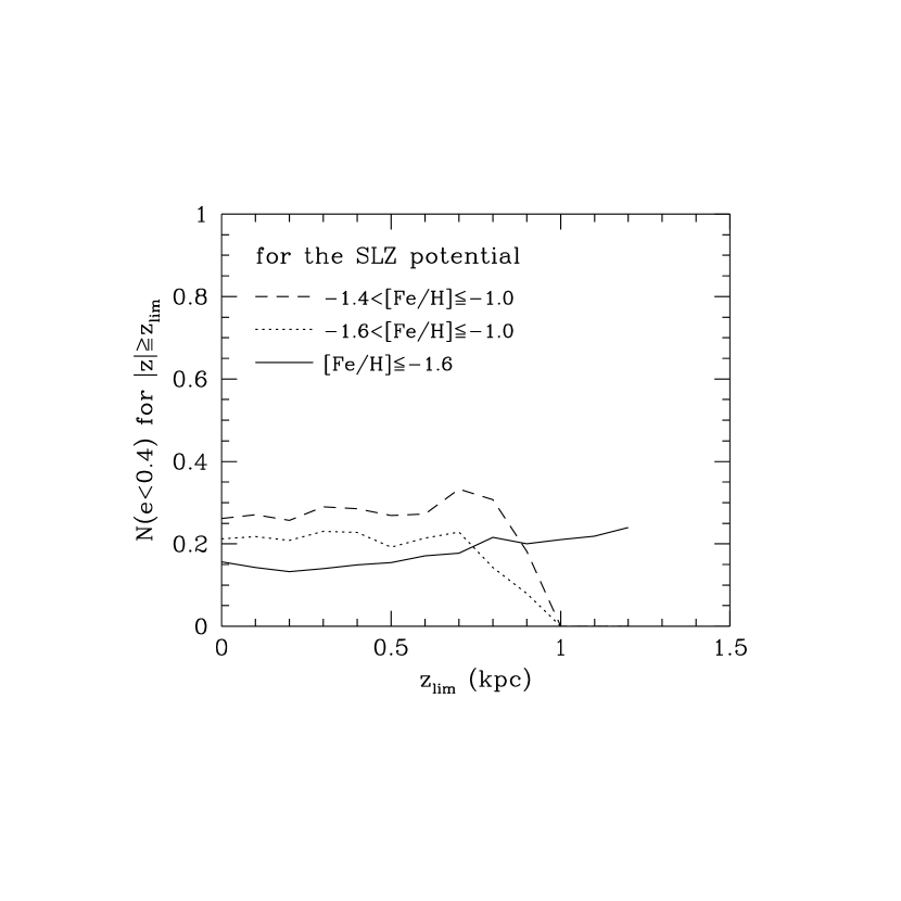
Figure 15: The fraction of stars having $e<0.4$ for $|z|\geq z_{lim}$, as a function of $z_{lim}$. Solid, dotted, and dashed lines are for [Fe/H]$\leq-1.6$, $-1.6<$[Fe/H]$\leq-1$, and $-1.4<$[Fe/H]$\leq-1$, respectively. Note the sharp decrease of the curves at $z_{lim}=0.8-1$ kpc for the intermediate metallicity range, whereas the curve for [Fe/H]$\leq-1.6$ remains essentially unchanged at large $z_{lim}$.

More direct insight into the vertical extent of the MWTD is obtained from Fig. 15 where the fraction of stars having $e<0.4$ is shown as a function of the limiting height $z_{lim}$ above or below which the stars are located, i.e., $|z|\geq z_{lim}$. This fraction sharply drops at $z_{lim}=0.8-1$ kpc for stars with $-1.6<$[Fe/H]$\leq-1$ (dotted line) or $-1.4<$[Fe/H]$\leq-1$ (dashed line), whereas it is kept almost constant for stars with [Fe/H]$\leq-1.6$ (solid line). Thus, the rapidly rotating MWTD component, which we have identified in the metal-poor range of $-1.6<$[Fe/H]$\leq-1$, have an vertical extent of $0.8-1$ kpc. This is virtually consistent with current estimates of the thick-disk scale height (e.g., Yoshii, Ishida, & Stobie 1987). It should also be noted that the halo component which is exclusively represented by stars with [Fe/H]$\leq-1.6$ shows no significant $z_{lim}$-dependence (solid line) and no noticeable contamination from the rapidly rotating MWTD. The low-$e$ fraction for [Fe/H]$\leq-1.6$ slightly increases towards higher $z_{lim}$. This may be explained from the fact that a star locating further out from the solar neighborhood has a smaller radial range in its orbital motion when a set of integrals of motion is given (Yoshii & Saio 1979).

5 Metallicity gradient as a clue to formation history

5.1 Introduction

Whether the Galaxy has a global metallicity gradient has been another key issue for understanding its early evolution. ELS used the $|W|$ velocity as an indicator of the maximum vertical height $|z_{max}|$ that stars can reach, and the ultraviolet excess $\delta(U-B)$ as an indicator of the metallicity corresponding to the epoch at which stars were born from the gas. ELS therefore argued that the correlation between $\delta(U-B)$ and $|W|$ may have arisen if the more metal-poor, older populations were formed at systematically larger heights beyond the disk, in other words, the Galaxy may have collapsed from an extended gas sphere to the disk.

Their argument implies that presence or absence of a large-scale metallicity gradient depends on the balance of competing time scales among the collapse of the Galaxy, the metal enrichment, and the spatial mixing of heavy elements in the gas (see also Sandage & Fouts 1987). In the free-falling proto-Galaxy via dissipation, the gas was progressively confined to smaller volumes, while newly formed stars were left over out of this infalling gas. This indicates higher metallicity for stars that were formed within smaller volumes, thereby causing the metallicity gradient. On the contrary, if the Galaxy was formed in a discontinuous or inhomogeneous manner, e.g., by merging of numerous fragments such as dwarf-type galaxies which have their own chemical histories (SZ), no global metallicity gradient would be observed in any spatial directions.

Figure 4 has already shown that a monotonous increase of the $|W|$-velocity with decreasing [Fe/H] is only detectable at [Fe/H]$>-1.4$ but not apparent at [Fe/H]$<-1.4$. It is important to here caution that the $|W|$-velocity alone does not characterize $|z_{max}|$ in a three-dimensional gravitational potential. As we demonstrate graphically in Fig. 16, our sample stars observed in the solar neighborhood have traveled through more distant regions of the Galaxy. For instance a star now at $(R,z)\sim(8.6,-0.5)$ kpc can orbit in the accessible area enclosed by solid line, whereas a star at $(R,z)\sim(8.6,0.0)$ kpc within the dotted-line area. Since the orbital $z$-motion is coupled with those in the $R$ and $\phi$ directions, $|W|$ is not necessarily related with $|z_{max}|$, especially for stars having large $|W|$-velocity or large asymmetric drift (see Carney et al. 1990).

We estimate the maximum height $|z_{max}|$ and the apogalactic cylindrical distance $R_{max}$ for each star using SLZ’s gravitational potential, and then examine how the estimates of $|z_{max}|$ and $R_{max}$ for our sample stars are related with their metal abundances. We first divide our sample into four $V_{\phi}$ bins of $V_{\phi}\leq\infty$, 170 km s^-1, 120 km s^-1, and 70 km s^-1. The halo component among various populations is extracted simply by selecting stars with small azimuthal velocity $V_{\phi}$ (Sandage & Fouts 1987; Carney et al. 1990, see also Sec. 3). However it is admittedly more problematic to discriminate the MWTD component alone. If we select large-$V_{\phi}$ stars assuming that the MWTD is rapidly rotating, the resultant sample will be considerably contaminated by the old disk component of metal-rich stars with [Fe/H]$>-0.6$. To avoid such a sampling bias, we attempt to discriminate the MWTD component from the small-$V_{\phi}$ halo component. We take advantage of the result in Sec. 4 that the MWTD stars likely have smaller $e$ compared to the halo stars and that their vertical distribution is confined within $|z|<1$ kpc. Accordingly we impose additional constraints of $e\leq 0.6$ and $|z|<1$ kpc to discriminate the MWTD from the halo component.

5.2 Results

Plots of [Fe/H] against $R_{max}$ and similar plots against $|z_{max}|$ are shown in Figs. 17 and 18, respectively, for ($a$) $V_{\phi}\leq\infty$ or all stars, ($b$) $V_{\phi}\leq 170$ km s^-1, and ($c$) $V_{\phi}\leq 120$ km s^-1. Note that the $V_{\phi}$ criteria used in panels $b$ and $c$ have successfully selecting halo stars with [Fe/H]$<-1$. The mean metal abundances in five bins of $R_{max}$ and in six bins of $|z_{max}|$ are connected by solid lines with estimated 1$\sigma$ errors of the means. These data are tabulated in Tables 7 and 8, where the results for $V_{\phi}\leq 70$ km s^-1 are also tabulated. These figures and tables clearly indicate that stars with $V_{\phi}\leq 170$ or $120$ km s^-1 show no large-scale metallicity gradient in the $R$ and $z$ directions within a 1$\sigma$ error level. This agrees with prior works based on different samples of field stars (Saha 1985; Carney et al. 1990) and halo globular clusters (Zinn 1985).

Figures 19 and 20 show the results for the MWTD candidate stars. We find that the additional constraints of $e\leq 0.6$ and $|z|<1$ kpc are effective for excluding the very metal-poor stars with [Fe/H]$<-1.8$. In contrast to the halo component as discussed above, there is an indication of a metallicity gradient $\Delta[Fe/H]/\Delta R_{max}=-0.03\sim-0.02$ dex kpc^-1 from $R_{max}=7$ to 18 kpc, and $\Delta[Fe/H]/\Delta|z_{max}|=-0.07\sim-0.05$ dex kpc^-1 from $|z_{max}|=1$ to 8 kpc. The number of the MWTD candidates may not be large enough to give a statistically significant result (see Tables 7 and 8), however it is intriguing to note that the obtained metallicity gradient is larger than the gradient previously detected from the thick-disk stars with [Fe/H]$\geq-1$ (e.g., Majewski 1993 for review). Further studies based on the assembly of more sample stars shall be important to elucidate this discrepancy and clarify the formation process of this controversial component.

6 DISCUSSION AND CONCLUSION

We have investigated the kinematics of 122 red giants and 124 RR Lyraes, which were selected without kinematic bias and were observed by the Hipparcos satellite to measure their accurate proper motions. The metal abundances of our program stars range from [Fe/H]$=-1$ to $-3$, thereby suitable for analyzing the halo component as well as the metal-weak tail of the thick disk component below [Fe/H]$=-1$. We summarize the obtained results below and discussed them in the light of the early evolution of the Galaxy.

6.1 Summary of the results

The present analyses indicate that the solar-neighborhood stars with [Fe/H]$\leq-1$ mostly have the halo-like kinematics of large velocity dispersion and no significant rotation. The velocity ellipsoid is radially elongated yielding $(\sigma_{U},\sigma_{V},\sigma_{W})=(161,115,108)$ km s^-1 in the metal-poor range of [Fe/H]$\leq-1.6$. The rotational properties of the system probed by $<V_{\phi}>$ or $<V_{\phi}>/\sigma_{\phi}$ appear to change largely at [Fe/H]$=-1.4\sim-1$ (Fig. 5), indicating that the collapse of the Galaxy from the halo to the disk took place discontinuously.

We have found no correlation between [Fe/H] and $e$ for [Fe/H]$\leq-1$ (Fig. 8), which is in contrast to the ELS result. Even for [Fe/H]$\leq-1.6$, about 16% of our program stars are found to have $e<0.4$ (the value of $e$ slightly depends on the gravitational potential adopted), and this fraction of low-$e$ stars stems from the radially elongated velocity ellipsoid of the halo component alone, without introducing an extra disk component (Figs. 9 and 10). Thus, the existence of low-$e$ stars does not necessarily mean the dominance of an extra rapidly-rotating component in the metal-poor range of [Fe/H]$\leq-1.6$. The conclusion that almost all stars with [Fe/H]$\leq-1.6$ belong to the halo component is supported by no significant change of the $e$ distribution with increasing $|z|$ (Figs. 14$a$ and 15). We have also found no large-scale metallicity gradient in the halo in both radial and vertical directions (Figs. 17 and 18).

Many workers claimed the metal-weak tail of the thick disk component in the range of $-1.6<$[Fe/H]$\leq-1$ (MFF; Beers & Sommer-Larsen 1995). The fraction of this component $F$ is however found to be smaller than previously thought. The maximum likelihood technique to fit to the observed $V_{\phi}$ distribution provides $F\sim 0.1$ for $-1.6<$[Fe/H]$\leq-1$ and $F\sim 0.2$ for $-1.4<$[Fe/H]$\leq-1$, while $F\sim 0$ for [Fe/H]$\leq-1.6$. We have shown that the distribution of orbital eccentricity provides a powerful method for constraining the fraction $F\approx 0.1-0.2$, the mean velocity $<V_{\phi}>_{disk}\approx 195$ km s^-1, and the vertical extent $z_{lim}\approx 0.8-1$ kpc of this extra disk component (Figs. $13-15$). We emphasize that this new approach is effective only if accurate proper motions are available by the astrometric satellite like Hipparcos.

We conclude from our results that the extra metal-weak disk which we have identified is the metal-weak tail of the rapidly rotating thick disk which dominates in the range of [Fe/H]$=-0.6$ to $-1$. This is therefore consistent with the claim by MFF and Beers and Sommer-Larsen (1995), although our estimate of $F\approx 0.1-0.2$ is much smaller than theirs. Using a full knowledge of the orbital motions of these disk-like stars, we have obtained possible indication of the large-scale metallicity gradient in the metal-weak tail of the thick disk component (Figs. 19 and 20).

6.2 Implications for the picture of Galaxy formation

6.2.1 The halo component

Our finding of no significant [Fe/H]$-e$ relation in the range of [Fe/H]$\leq-1.6$ conflicts with the ELS scenario that the the proto-Galaxy underwent the free-fall collapse and the formed stars out of the falling gas should have eccentric orbits. The presence of low-$e$ halo stars in our sample, although comprising only a small fraction, is a key for understanding how the halo was formed because such low-$e$ stars belong to the halo, but not to the rapidly rotating thick disk.

Our program stars were sampled in the vicinity of the Sun and only about 16% of the sample have eccentricities below $e=0.4$. As a direct consequence of the radially elongated velocity ellipsoid, the $e$ distribution is largely skewed towards higher $e$. On the other hand, the orbital motions of halo stars sampled at much larger galactocentric distances remain yet undetermined because of the lack of accurate measurements of their proper motions. However, an intriguing result on the velocity distribution in the outer halo has been derived by Sommer-Larsen et al. (1994) using the radial velocities for their sample of blue horizontal branch stars at $r=5-55$ kpc. Their analyses indicate that the velocity ellipsoid turns out to be tangentially anisotropic beyond $r\sim 15$ kpc. This implies that high angular momentum, small-$e$ orbits are dominant in the outer halo (bold dashed lines in Figs. 9 and 10). Thus, any scenarios for the formation of the Galaxy must explain not only the $e$ distribution in the solar neighborhood but also the the velocity ellipsoid with radial anisotropy transforming into tangential anisotropy with increasing galactocentric distance.

If one adopts the currently favored SZ scenario that the halo was assembled from merging or accretion of numerous fragments, no correlation between kinematical and chemical properties is expected, because each fragment, presumably a gas-rich or gas-poor dwarf-type galaxy, has its own chemical history. The SZ scenario is thus successful in explaining no [Fe/H]$-e$ relation and no global metallicity gradient derived from the halo stars observed near the Sun. It is also consistent with a wide age spread in globular clusters as well as in field stars, because star formation in each fragment proceeds independently.

We proceed to ask whether the SZ scenario is furthermore consistent with the $e$ distribution in the solar neighborhood and the change of the velocity ellipsoid with increasing galactrocentric distance. A process of merging or accretion of dwarf-type galaxies involves dynamical friction which reduces its orbital radius (e.g. Quinn et al. 1993). At some radius below which the mean density of the fragment is exceeded by the mean density of the Galaxy, the fragment is tidally disrupted and the debris is dispersed to constitute the stellar halo. Since the dynamical friction tends to circularize the orbit of the fragment, the orbits of remnant stars are weighted in favor of small $e$. This indicates that the velocity ellipsoid becomes more tangentially anisotropic at smaller galactocentric distance, which is opposite to the observed trend. Although detailed numerical simulations of modeling a number of accreting events are to be explored, the above simple argument implies that the SZ scenario seems unlikely to reproduce the kinematical properties of halo stars.

An alternative scenario of the formation of the Galaxy has been proposed by Sommer-Larsen and Christensen (1989) to explain the change of the velocity ellipsoid with galactrocentric distance. When the proto-Galactic overdense region started to collapse out of cosmological expansion, large fluctuations developed within the mixture of gas and dark matters made the gas heated up to the virial temperature of about $10^{6}$ K (which is typical of the Galaxy). This virialized system is largely pressure-supported inside the virial radius. Ensembles of gas clouds are isotropically moving at each radius, and dissipative cloud-cloud collisions then induces formation of halo stars. The collision rate is orbit-dependent. For example, clouds having more radially eccentric orbits encounter with more clouds in denser inner parts of the Galaxy, so that such clouds may never return to the radius from which the orbital motions start. Thus, this mechanism favors the survival of systematically more circular orbits at larger radii, which agrees with the kinematical properties of halo stars.

This scenario was further investigated by Theis (1996) performing numerical simulations of collapsing dissipative cloud system. He has successfully obtained the tangentially elongated velocity ellipsoid for survived clouds after the dissipative collapse. It is however yet unexplored whether stars formed by this mechanism have the same kinematical and chemical properties as observed. Specifically, since the mechanism involves gaseous dissipation over several free-fall time scales, a large-scale metallicity gradient may appear in the stellar system. In this respect, the effects of energy feedback from massive stellar winds and supernovae explosions to the surrounding gas may play an important role in suppressing rapid gaseous dissipation and smearing out any metallicity gradient by rapid mixing of heavy elements in the gas.

The more realistic picture is in between the above scenarios. The currently favored cold-dark-matter scenario of galaxy formation indicates that the initial density fluctuations in the early Universe have larger amplitudes on smaller scales (e.g., Padmanabhan 1993). Hence, the initial overdense regions that end up with giant galaxies like our own contain larger density fluctuations on sub-galactic scales. In a collapsing protogalaxy these small-scale fluctuations develop to numerous fragments which interact together via gravitational force (Katz & Gunn 1991). Due to torque among fragments or direct merging, angular momentum is transferred from inner to outer regions of the system. Since star formation and chemical evolution differently progress in each fragment, one might expect a wide age spread and no metallicity gradient in the final stellar system. This is indeed indistinguishable from the SZ scenario. If halo stars are formed via inelastic, anisotropic collisional processes between fragments, the kinematics of such stars may well accord with the observed transition of the velocity ellipsoid from the solar neighborhood to the outer halo (Sommer-Larsen & Christensen 1989).

Some of the small density contrasts that have gained systematically higher angular momentum in the course of cosmological expansion may have slowly fallen to the system after most parts of the system were settled. These delayed accretion may explain the reported indications of relatively young stars (Rodgers et al. 1981) and retrograde-orbit stars (Majewski 1992) in the outer halo, which have been regarded as a direct evidence of accretion. It is indeed of great importance to investigate this scenario in more detail, by exploring high-resolution simulations of collapsing galaxy combined with star formation and chemical evolution, in order to fully understand the kinematical and chemical properties of the halo reported in the present work.

6.2.2 The thick disk component

How the disk with a large vertical scale height was formed is also enigmatic (e.g., Majewski 1993). One leading scenario is that the disk was heated by the merging of satellites with the preexisting thin disk (Quinn et al. 1993). Satellite orbits were decayed and circularized into the disk plane, and then fallen towards the center of the disk. The disk stars were spread out by the merging, and the aftermath was reported to be similar to the observed spatial structure and kinematical properties of the thick disk component. According to this scenario the thin disk was formed after a major merger event. Therefore, timing of this merger event is severely constrained by the presence of the presently observed thin disk with a vertical scale height of 350 pc. An alternative scenario is that the thick disk may have formed in a dissipative manner after the major parts of the halo formation were completed (e.g., Larson 1976; Burkert et al. 1992; Burkert & Yoshii 1996). Contraction of the disk either occurred in a pressure-supported manner because of the energy feedback or rapidly progressed into the thin disk because of the efficient line cooling.

One of the possible observational clues to discriminate these scenarios lies in the fraction of the thick disk in the metal-poor range of [Fe/H]$\leq-1.6$. In the merger scenario, since the mechanism relies on both the preexisting old disk and merging satellites having different chemical histories, the aftermath of the merger may contain numerous metal-poor stars. On the contrary, in the dissipative-collapse scenario, since the gas that forms the thick disk is already enriched by metal ejection of halo stars, only few metal-poor stars should be observed in the thick disk. Our finding of essentially no thick-disk stars in the range of [Fe/H]$\leq-1.6$ appears to support the latter scenario.

Another clue to clarify the formation of the thick disk is to examine whether a large-scale metallicity gradient exists. The merger scenario may envisage no metallicity gradient, whereas the dissipative contraction of the disk may involve the smooth spatial variation of metallicity in stars. No consensus has ever met on the observational evidence of metallicity gradient in the thick disk (Majewski 1993). However, if our finding of non-negligible metallicity gradient in the metal-weak disk is the case, it is possible to deduce that the contraction of the halo into the thick disk occurred in a dissipative manner just after the major parts of the halo formation were completed.

Before concluding definitely, it is required to assemble the data of more stars having accurate distances and proper motions. The method that we have developed here based on the eccentricity distribution of orbits may be useful for examining whether the thick disk has a significant metal-weak tail as well as a global metallicity gradient. More elaborate modelings are needed to further clarify the physical connection between the halo and the thick disk and to propose what observation will be most definite discriminator of the scenario of the formation of the Galaxy.

Appendix A The ELS model for the gravitational potential

The ELS potential as a function of galactocentric distance $R$ in the plane is given by

$$\Phi_{ELS}(R)=-\frac{GM}{b+(R^{2}+b^{2})^{1/2}}\ ,$$ (A1)

where $M$ is the total mass of the disk and $b$ is the scale length. In the centrifugal equilibrium of the disk, the circular velocity $V_{c}$ is given by $V_{c}(R)=[Rd\Phi_{ELS}/dR]^{1/2}$.

The values of $b$ and $M$ can be evaluated from the Oort constants ($A$,$B$) and the circular velocity $V_{\odot}$ at $R_{\odot}$ , i.e.,

$$-\frac{A+B}{A-B} = \frac{1+2q-q^{2}}{2q^{2}}$$ (A2)

$$V_{c}(R_{\odot}) = V_{\odot}\ ,$$ (A3)

where $q\equiv[(R_{\odot}/b)^{2}+1]^{1/2}$. For $A=15$ km s^-1 kpc^-1 and $B=-10$ km s^-1 kpc^-1, eq. (A2) gives $q=3.77$ and thus $b=R_{\odot}/3.65$ kpc. Equation (A3) then reads $(GM/b)^{1/2}=2.54V_{\odot}$. ELS adopted $R_{\odot}=10$ kpc and $V_{\odot}=250$ km s^-1, thereby $b=2.74$ kpc and $(GM/b)^{1/2}=635$ km s^-1. If $R_{\odot}=8$ kpc and $V_{\odot}=220$ km s^-1 as adopted by Carney et al. (1990), we obtain $b=2.19$ kpc and $(GM/b)^{1/2}=559$ km s^-1.

In the present work, we use the escape velocity $V_{esc}$ near the Sun as an alternative constraint. The definition $V_{esc}=[2|\Phi_{ELS}(R_{\odot})|]^{1/2}$ then reads

$$1-\left(\frac{\sqrt{2}V_{\odot}}{V_{esc}}\right)^{2}=\frac{1}{q}\ ,$$ (A4)

instead of eq. (A2). For $V_{\odot}=220$ km s^-1 and $V_{esc}=450$ km s^-1, we obtain $q=1.92$, thus $b=R_{\odot}/1.63=5.2$ kpc. Equation (A3) then reads $(GM/b)^{1/2}=2.48V_{\odot}=545$ km s^-1 for $V_{\odot}=220$ km s^-1. This model is characterized by the larger $b$ than previous ones to accord with the large $V_{esc}$ as observed near the Sun.

TABLE 4

Rotational Properties of the Sample Stars

[Fe/H]	$<$[Fe/H]$>$	$N$	$<V_{\phi}>$	$\sigma_{\phi}$	$<V_{\phi}>/\sigma_{\phi}$
(dex)	(dex)		(km/s)	(km/s)
$+0.10$ to $-0.50$	$-0.20$	5	$205\pm 7$	$26\pm 9$	$7.97\pm 2.83$
$-0.50$ to $-0.90$	$-0.70$	9	$172\pm 13$	$48\pm 12$	$3.61\pm 0.94$
$-0.90$ to $-1.28$	$-1.09$	22	$56\pm 11$	$84\pm 13$	$0.66\pm 0.17$
$-1.28$ to $-1.45$	$-1.37$	21	$39\pm 16$	$108\pm 17$	$0.36\pm 0.16$
$-1.45$ to $-1.56$	$-1.50$	18	$18\pm 17$	$107\pm 18$	$0.17\pm 0.17$
$-1.56$ to $-1.75$	$-1.65$	36	$-7\pm 19$	$97\pm 12$	$-0.08\pm 0.20$
$-1.75$ to $-1.95$	$-1.85$	26	$27\pm 17$	$119\pm 17$	$0.22\pm 0.14$
$-1.95$ to $-2.30$	$-2.12$	33	$12\pm 20$	$115\pm 14$	$0.10\pm 0.17$
$-2.30$ to $-3.01$	$-2.65$	38	$-11\pm 19$	$122\pm 14$	$-0.09\pm 0.15$

Figure 1: The distribution of relative parallax errors $\sigma_{\pi}/\pi$. Filled and open circles denote red giants and RR Lyraes, respectively.

Figure 2: The difference between the previous (superscript ’old’) and the Hipparcos (’HIP’) measurements for proper motions $\mu_{\alpha^{\ast}}$ (a) and $\mu_{\delta}$ (b). Filled and open circles denote red giants and RR Lyraes, respectively, with small relative errors in proper motions ($|\mu_{\alpha^{\ast}}|>\sigma_{\mu_{\alpha^{\ast}}}$ and $|\mu_{\delta}|>\sigma_{\mu_{\delta}}$), while filled and open triangles are for large errors ($|\mu_{\alpha^{\ast}}|\leq\sigma_{\mu_{\alpha^{\ast}}}$ or $|\mu_{\delta}|\leq\sigma_{\mu_{\delta}}$).

Figure 3: The distributions of distances (a) and metallicities (b) for red giants (shaded histograms) and RR Lyraes (solid histograms). In panel $b$, dotted histogram is for both stars, while solid line shows the likely true metallicity distribution of halo stars derived by Laird et al. (1988).

Figure 4: $(U,V,W)$ velocity components versus [Fe/H] for the sample. The symbol designation is the same as in Fig. 2.

Figure 5: Rotational properties versus [Fe/H] for the sample. (a) The mean rotation $<V_{\phi}>$. (b) The velocity dispersion in $\phi$ direction, $\sigma_{\phi}$. (c) The ratio $<V_{\phi}>/\sigma_{\phi}$.

Figure 6: The distributions of $V_{\phi}$ in various metallicity ranges for red giants (solid lines) and RR Lyraes (dotted lines). The left and right panels are for $|z|<1$ kpc and $|z|\geq 1$ kpc, respectively, and the metallicity ranges are indicated in the labels for vertical axes. Note that in the range of $-1.6\leq$[Fe/H]$\leq-1$ (panel $c$), the deviation from a single Gaussian is less significant than previously reported.

Figure 7: The results of the maximum likelihood method for reproducing the $V_{\phi}$ distribution at $|z|<1$ kpc, based on a mixture of two Gaussian components (halo$+$disk). The mean rotation of the disk $<V_{\phi}>_{disk}$ is one of the variable parameters for fitting. The metallicity ranges are $-1.6<$[Fe/H]$\leq-1$ (panels $a$, $d$, and $g$), $-1.5<$[Fe/H]$\leq-1$ (panels $b$, $e$, and $h$), and $-1.4<$[Fe/H]$\leq-1$ (panels $c$, $f$, and $i$).

Figure 8: The relation between [Fe/H] and $e$ for the ELS (a) and the SLZ (b) gravitational potentials. The symbol designation is the same as in Fig. 2.

Figure 9: The normalized differential $e$ distribution $n(e)$ for the sample stars with [Fe/H]$\leq-1.6$ (solid histograms) and $-1.6<$[Fe/H]$\leq-1$ (dotted histograms). Bold solid (model A) and bold dashed lines (model B) denote the model predictions based on a single Gaussian velocity distribution with a radially anisotropic $(\sigma_{U},\sigma_{V},\sigma_{W})=(161,115,108)$ km s^-1 and a tangentially anisotropic $(115,161,108)$ km s^-1 velocity ellipsoid, respectively. The former velocity ellipsoid is derived from stars with [Fe/H]$\leq-1.6$, whereas the latter one is just for the purpose of comparison.

Figure 10: The cumulative $e$ distribution $N(<e)$ for the sample. Others are the same as for Fig. 9.

Figure 11: The Bottlinger diagram for the sample stars. The symbol designation is the same as in Fig. 2. Each curve denotes a locus of constant $e$ derived from the ELS gravitational potential.

Figure 12: The distribution of errors $\sigma_{e}$ in $e$ for the ELS gravitational potential.

Figure 13: The cumulative $e$ distribution for the stars at $|z|<$1 kpc, in the metallicity ranges of [Fe/H]$\leq-1.6$ (solid histograms), $-1.6<$[Fe/H]$\leq-1$ (dotted histograms), and $-1.4<$[Fe/H]$\leq-1$ (dashed histograms). The SLZ gravitational potential is used. Bold solid line in panel $a$ corresponds to the model prediction using the velocity ellipsoid $(\sigma_{U},\sigma_{V},\sigma_{W})=(165,120,107)$ km s^-1 obtained for stars at $|z|<1$ kpc with [Fe/H]$<-1.6$. Various bold lines in panels $b$ and $c$ denote the model results based on a mixture of two Gaussian components (thick disk$+$halo). The quantity $F$ denotes the fraction of the thick-disk component. Panel $b$ is for the mean disk rotation of $<V_{\phi}>_{disk}=195$ km s^-1, while panel $c$ is for $<V_{\phi}>_{disk}=120$ km s^-1.

Figure 14: (a) The normalized cumulative $e$ distribution for stars at $|z|\geq$1 kpc. Bold solid line is the same as that (model A) in Fig. 10. Others are the same as for Fig. 10. (b) The relation between [Fe/H] and $e$ at $|z|\geq 1$ kpc for the SLZ gravitational potential. Note that when comparing with Fig. 8 for all $z$, stars enclosed by dotted lines are selectively excluded by the constraint $|z|\geq 1$ kpc.

Figure 16: The spatial distribution of the sample stars in $(R,z)$. The area enclosed by solid lines corresponds to the domain of orbital motions for HIC#3554 at $(R,z)=(8.58,-0.54)$ kpc, whereas dotted lines are for HIC#2413 at $(R,z)=(8.62,-0.02)$ kpc. The SLZ gravitational model is used.

Figure 17: The relation between [Fe/H] and $R_{max}$ for the sample (crosses) with $V_{\phi}\leq\infty$ (a), $V_{\phi}\leq 170$ km s^-1 (b), and $V_{\phi}\leq 120$ km s^-1 (c). Error bars denote the mean [Fe/H] and $1\sigma$ errors obtained in different ranges of $R_{max}$ as tabulated in Table 7, and bold solid lines trace the mean [Fe/H]. The SLZ gravitational model is used.

Figure 18: The relation between [Fe/H] and $|z_{max}|$ for the sample (crosses). Error bars denote the mean [Fe/H] and $1\sigma$ errors obtained in different ranges of $|z_{max}|$ as tabulated in Table 8. Others are the same as for Fig. 17.

Figure 19: The same as in Fig. 17, but for the MWTD candidate stars selected from the additional constraints of $e\leq 0.6$ and $|z|<1$ kpc.

Figure 20: The same as in Fig. 19, but for [Fe/H] versus $|z_{max}|$.

References

- (1) Anthony-Twarog, B. J. & Twarog, B. A. 1994, AJ, 107, 1577 (ATT)
- (2) Bahcall, J. N., Schmidt, M., & Soneira, R., M. 1982, ApJ, 258, L23
- (3) Barbier-Brossat, M. 1989, A&ASuppl., 80, 67
- (4) Beers, T. C. & Sommer-Larsen, J. 1995, ApJS, 96, 175
- (5) Blanco, V. M. 1992, AJ, 104, 734
- (6) Bond, H. E. 1980, ApJS, 44, 517
- (7) Burkert, A. & Yoshii, Y. 1996, MNRAS, 282, 1349
- (8) Burkert, A., Truran, J. W., & Hensler, G. 1992, ApJ, 391, 651
- (9) Burstein, D. & Heiles, C. 1982, AJ, 87, 1165
- (10) Carney, B. W. 1988, in The Harlow-Shapley Symposium on Globular Cluster Systems in Galaxies, ed. J. E. Grindlay & A. G. D. Philip (Dordrecht: Reidel), 133
- (11) Carney, B. W. & Latham, D. W. 1986, AJ, 92, 60
- (12) Carney, B. W., Aguilar, L, Latham, D. W., & Laird, J.B. 1990, AJ, 99, 201
- (13) Carney, B. W., Latham, D. W., & Laird, J.B. 1988, AJ, 96, 560
- (14) Carney, B. W., Latham, D. W., & Laird, J.B. 1990, AJ, 99, 572
- (15) Carney, B. W., Storm, J., & Jones, R. V. 1992, ApJ, 386, 663 (CSJ)
- (16) Clube, S. V. M. & Dawe, J. A. 1980, MNRAS, 190, 591
- (17) de Zeeuw, T., Peletier, R., & Franx, M. 1986, MNRAS, 221, 1001
- (18) Eggen, O. J., Lynden-Bell, D., & Sandage, A. R. 1962, ApJ, 136, 748 (ELS)
- (19) ESA 1997, The Hipparcos and Tycho Catalogues, ESA SP-1200, in press
- (20) Evans, D. S. 1978, Bull. Inf. CDS, 15 121
- (21) FitzGerald, M. P. 1968, AJ, 73, 983
- (22) FitzGerald, M. P. 1987, MNRAS, 229, 227
- (23) Freeman, K. C. 1987, ARA&A, 25, 603
- (24) Gilmore, G. & Reid, I. N. 1983, MNRAS, 202, 1025
- (25) Griffin, R., Griffin, R., Gustafsson, B., & Vieira, T. 1982, MNRAS, 198, 637
- (26) Johnson, D. R. H. & Soderblom, D. R. 1987, AJ, 93, 864
- (27) Katz, N. & Gunn, J. E. 1991, ApJ, 377, 365
- (28) Klemola, A. R., Hanson, R. B., & Jones, B. F. 1993, Lick Northern Proper Motion Program: NPM1 Catalog, National Space Science Data Center – Astronomical Data Center Catalog No. A1199
- (29) Kukarkin, B. V. et al. 1969-1976, General Catalogue of Variable Stars, 3rd ed., 3 volumes and 3 supplements (The Moscow State University, Moscow)
- (30) Laird, J. B., Rupen, M. P., Carney, B. W., & Latham, D. W. 1988, AJ, 96, 1908
- (31) Lanzetta, K. M., Wolfe, A. M., & Turnshek, D. A. 1995, ApJ, 440, 435
- (32) Larson, R. B. 1976, MNRAS, 170, 31
- (33) Layden, A. C. 1994, AJ, 108, 1016
- (34) Layden, A. C. 1995, AJ, 110, 2288
- (35) Layden, A. C. 1996, AJ, 112, 2110
- (36) Lu, L. et al. 1996, ApJS, 107, 475
- (37) Majewski, S. R. 1992, ApJS, 78, 87
- (38) Majewski, S. R. 1993, ARA&A, 31, 575
- (39) Mihalas, D. & Binney, J. 1981, Galactic Astronomy (San Francisco: Freeman)
- (40) Morrison, H. L., Flynn, C., & Freeman, K. C. 1990, AJ, 100, 1191 (MFF)
- (41) Norris, J. E. 1986, ApJS, 61, 667
- (42) Norris, J. E. 1996, in Formation of the Galactic Halo … Inside and Out, ed. H. Morrison & A. Sarajedini (ASP Conf. Ser. 92), 14
- (43) Norris, J. E. & Ryan, S. G. 1989, ApJ, 349, 739
- (44) Norris, J. E. & Ryan, S. G. 1991, ApJ, 380, 403
- (45) Norris, J. E., Bessell, M. S., & Pickles, A. J. 1985, ApJS, 58, 463 (NBP)
- (46) Padmanabhan, T. 1993, Structure Formation in the Universe (Cambridge: Cambridge Univ. Press)
- (47) Perryman, M. A. C. et al. 1995, A&A, 304, 69
- (48) Pettini, M., King, D. L., Smith, L. J., & Hunstead, .R. W. 1995, in QSO Absorption Lines, ed. G. Meylan (Berlin: Springer), 71
- (49) Quinn, P. J., Hernquist, L., & Fullagar, D. P. 1993, ApJ, 403, 74
- (50) Rodgers, A. W. & Roberts, W. H. 1993, AJ, 106, 1839
- (51) Rodgers, A. W. et al. 1981, ApJ, 244, 912
- (52) Ryan, S. G. & Norris, J. E. 1991, AJ, 101, 1865
- (53) Ryan, S. G. & Lambert, D. L. 1995, AJ, 109, 2068
- (54) Saha, A. 1985, ApJ, 289, 310
- (55) Sandage, A. R. 1993, AJ, 106, 703
- (56) Sandage, A. R. & Fouts, G. 1987, AJ, 93, 74
- (57) Schuster, W. J. & Nissen, P. E. 1989, A&A, 222, 69
- (58) Searle, L. & Zinn, R. 1978, ApJ, 225, 357 (SZ)
- (59) Sommer-Larsen, J. & Christensen, P. R. 1989, MNRAS, 239, 441
- (60) Sommer-Larsen, J. & Zhen, C. 1990, MNRAS, 242, 10 (SLZ)
- (61) Sommer-Larsen, J., Flynn, C., & Christensen, P. R. 1994, MNRAS, 271, 94
- (62) Theis, C. 1996, in The History of the Milky Way and Its Satellite System, ed. A. Burkert, D. H. Hartmann, & S. R. Majewski (ASP Conf. Ser. 112), 35
- (63) Turon, C. et al. 1992, The Hipparcos Input Catalogue, ESA SP-1136, 7 volumes.
- (64) Twarog, B. A. & Anthony-Twarog, B. J. 1994, AJ, 107, 1371
- (65) Twarog, B. A. & Anthony-Twarog, B. J. 1996, AJ, 111, 220
- (66) Vogt, N. P. et al. 1996, ApJ, 465, L15
- (67) Wan, L., Mao, Y.-Q., & Ji, D.-S. 1980, Ann. Shanghai Obs., No. 2, 1
- (68) Wilhelm, R. 1995, Ph.D. Thesis, Michigan State University
- (69) Williams, R E. et al. 1996, AJ, 112, 1335
- (70) Wilson, R. E. 1953, General Catalogue of Stellar Radial Velocities, Carnegie Institution of Washington Publ. 601
- (71) Yoshii, Y. 1982, PASJ, 34, 365
- (72) Yoshii, Y. & Saio, H. 1979, PASJ, 31, 339
- (73) Yoshii, Y., Ishida, K., & Stobie, R. S. 1987, AJ, 323
- (74) Zinn, R. 1985, ApJ, 293, 424
- (75) Zinn, R. 1988, in The Harlow-Shapley Symposium on Globular Cluster Systems in Galaxies, ed. J. E. Grindlay & A. G. D. Philip (Dordrecht: Reidel), 37
- (76) Zinn, R. & West, M. J. 1984, ApJS, 55, 45
TABLE 2
Literature Sources