The art of fitting p-mode spectra: Part II. Leakage and noise covariance matrices

Abstract

In Part I we have developed a theory for fitting p-mode Fourier spectra assuming that these spectra have a multi-normal distribution. We showed, using Monte-Carlo simulations, how one can obtain p-mode parameters using ’Maximum Likelihood Estimators’. In this article, hereafter Part II, we show how to use the theory developed in Part I for fitting real data. We introduce 4 new diagnostics in helioseismology: the $(m,\nu)$ echelle diagramme, the cross echelle diagramme, the inter echelle diagramme, and the ratio cross spectrum. These diagnostics are extremely powerful to visualize and understand the covariance matrices of the Fourier spectra, and also to find bugs in the data analysis code. These diagrammes can also be used to derive quantitative information on the mode leakage and noise covariance matrices. Numerous examples using the LOI/SOHO and GONG data are given.

1 Introduction

The physics of the solar interior is known from inversion of solar p-mode frequencies and splittings. These measurements are derived from fitting p-mode Fourier spectra. Schou (1992) was the first one to assume a multi-normal distribution for p-mode Fourier spectra and using a real leakage matrix. Following this pioneering work, Appourchaux et al. (1997) (hereafter Part I), generalized the theoretical background for fitting p-mode Fourier spectra to complex leakage matrix, and included explicitly the correlation of the noise between the Fourier spectra. Using Monte-Carlo simulations, we showed that our fitted parameters were unbiased. We also studied systematic errors due to an imperfect knowledge of the leakage covariance matrix. Unfortunately, a theoretical knowledge of fitting data is not enough as only real data will teach us if our approach is correct. Contrary to fitting p-mode power spectra, the process of fitting the Fourier spectra as described in Part I is rather difficult to understand and visualize. Schou (1992) gave a few diagnostics for understanding how the Fourier spectra are fitted but without showing an easy way to visualize the covariance matrices.

In this paper, we show how one can easily visualize the mode and noise correlation matrices, and then derive the mode leakage matrix. In the first section, we describe 4 new diagrammes that have various diagnostics power. In the second section, we describe how we use those diagrammes for inferring the leakage and noise covariance matrices for the data of the Luminosity Oscillations Imager (LOI) on board the Solar and Heliospheric Observatory (SOHO) data (Appourchaux et al, 1997), and for the data of the Global Oscillations Network Group (GONG) (Hill et al, 1996). The LOI time series starts on 27 March 1996 and ends on 27 March 1997 with a duty cycle greater than 99%. The GONG time series starts on 27 August 1995 and ends on 22 August 1996 with a 75% duty cycle. In the last section we conclude by emphasizing the usefulness of these diagrammes.

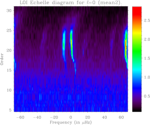
Figure 1: Amplitude spectra echelle diagramme for 1 year of LOI data seeing the Sun as a star. The scale is in part-per-million $\mu$Hz^-1/2 (ppm $\mu$Hz^-1/2). The spacing is tuned for $l=0$. The $l=0$ modes are at the center, the $l=2$ modes are about 10 $\mu$Hz on the left hand side, the $l=1$ modes are about +65 $\mu$Hz on the right hand side, the $l=3$ can be faintly seen at about 12 $\mu$Hz from the left hand side of the $l=1$. Other modes such as $l=4$ and $l=5$ can also be seen faintly seen at -35 $\mu$Hz and +15 $\mu$Hz, respectively. The distortion of the ridges are due to sound speed gradients in the solar core.

2 Diagnostics for helioseismic data analysis

The echelle diagramme was first introduced by Grec (1981). It is based on the fact that the low-degree modes are essentially equidistant in frequency for a given $l$; the typical spacing for $l=0$ is 136 $\mu$Hz. The spectrum is cut into pieces of 136 $\mu$Hz which are stacked on top of each other. Since the modes are not truly equidistant in frequency, the echelle diagramme shows up power as distorted ridges; an example is given in Fig. 1 for the LOI/SOHO instrument seeing the Sun as a star.

Another useful diagramme was introduced by Brown (1985), the so-called $(m,\nu)$ diagramme which shows how the frequency of an $l,m$ mode depends upon $m$. Most often this diagramme is only shown for a single $n$ and for intermediate degrees $l\geq 10$.

The purpose of these diagrammes is always to show an estimate of the variance of the spectra. In our case we also want to visualize not only the variance but also the covariance of the Fourier spectra. Here we briefly recall from Part I that the observed Fourier spectra ($\@vec{y}$) can be related to the individual Fourier spectra of the normal modes ($\@vec{x}$) by the leakage matrix $\@tens{\cal{C}}^{(l,l^{\prime})}$ by:

$$\@vec{y}=\@tens{\cal{C}}^{(l,l^{\prime})}\@vec{x}$$ (1)

The covariance matrix $\@tens{V}^{(l,l^{\prime})}_{m,m^{\prime}}$ of $\@vec{z}_{\@vec{y}}$ ($\@vec{z}_{\@vec{y}}^{\rm T}=(\mbox{Re}(\@vec{y}^{\rm T}),\mbox{Im}(\@vec{y}^{\rm T}))$), can be derived from the sub-matrix $\@tens{\cal{V}}^{(l,l^{\prime})}$ whose elements can be expressed as:

$$2\@tens{\cal{V}}^{(l,l^{\prime})}_{m,m^{\prime}}=E[y_{l,m}(\nu)y_{l^{\prime},m^{\prime}}^{*}(\nu)]=$$

$$2\sum_{l"=l,l^{\prime}}\sum_{m"=-l"}^{m"=l"}\@tens{\cal{C}}_{m^{\prime},m"}^{(l^{\prime},l")}\@tens{\cal{C}}_{m,m"}^{(l,l")*}f_{m"}^{l^{\prime\prime}}(\nu)+2\@tens{\cal{B}}_{m,m^{\prime}}^{(l,l^{\prime})}$$ (2)

where $E$ is the expectation, $f_{m^{\prime\prime}}^{l^{\prime\prime}}(\nu)$ is the profile of the $l^{\prime\prime},m^{\prime\prime}$ mode, $\@tens{\cal{B}}^{(l,l^{\prime})}$ is the covariance matrix of the noise, and with the $y_{l,m}(\nu)$ having a mean of zero. The factor 2 comes from the fact that the real part of $\@tens{\cal{V}}^{(l,l^{\prime})}$ represents both the covariance of the real or imaginary parts of the Fourier spectra (See Part I, section 3.3.2); the same property applied to the imaginary part of $\@tens{\cal{V}}^{(l,l^{\prime})}$ which represents the covariance between the real part and the imaginary part of the Fourier spectra. Equation (2) contains all the information that we need for visualizing an estimate of the real and imaginary parts of $\@tens{\cal{V}}^{(l,l^{\prime})}$. Drawing from the usefulness of the diagrammes of Grec and Brown, we created four new diagrammes for visualizing an estimate of $\@tens{\cal{V}}^{(l,l^{\prime})}$, all having various diagnostics power:

1. $(m,\nu)$ echelle diagramme: estimate of the diagonal elements of $\@tens{\cal{V}}^{(l,l)}$ ($l=l^{\prime}$)

2. cross echelle diagramme: estimate of the off-diagonal elements of $\@tens{\cal{V}}^{(l,l)}$ ($l=l^{\prime}$)

3. inter echelle diagramme: estimate of the off-diagonal elements of $\@tens{\cal{V}}^{(l,l^{\prime})}$ ($l/nel^{\prime}$)

4. ratio cross spectrum: estimate of the ratio of the elements of $\@tens{\cal{B}}^{(l,l^{\prime})}$

Each diagnostic is described hereafter in more detail.

2.1 $(m,\nu)$ echelle diagramme

The $(m,\nu)$ echelle diagramme is made of $2l+1$ echelle diagrammes of each $l,m$ power spectra or $|y_{l,m}(\nu)|^{2}$. The $2l+1$ echelle diagrammes are stacked on top of each other to show the dependence of the mode frequency upon $m$. These diagrammes give an estimate of the diagonal of the covariance matrix of the observations as:

$$2\widetilde{\@tens{\cal{V}}}_{m,m}^{(l,l)}(\nu)=|y_{l,m}(\nu)|^{2}$$ (3)

where $\widetilde{\@tens{\cal{V}}}^{(l,l)}$ symbolizes the estimate of $\@tens{\cal{V}}^{(l,l)}$. It is important when one makes these diagrammes to tune the spacing for the degree to study. The spacing for a given $l$ can be computed from available p-mode frequencies. Since the spacing varies with the degree, other modes with a significant different spacing can be seen more like diagonal ridges crossing the $(m,\nu)$ diagrammes; this is a powerful tool to identify other degrees.

Nevertheless, the diagnostics power of the $m,\nu$ echelle diagramme is rather limited for deriving the leakage matrix: it can be shown using Eq. (2) that the diagonal elements of $\@tens{\cal{V}}^{(l,l)}$ can be expressed as:

$$\@tens{\cal{V}}^{(l,l)}_{m,m}=\sum_{m"=-l}^{m"=l}|\@tens{\cal{C}}_{m,m"}^{(l,l)}|^{2}f_{m"}^{l}(\nu)+\@tens{\cal{B}}_{m,m}^{(l,l)}$$ (4)

As we can see with Eq. (4), the sign information of the elements of $\@tens{\cal{C}}^{(l,l)}$ is lost; second, their magnitude being typically less than 0.5, the leakage elements cannot be easily seen in the power spectra. Another kind of diagramme that preserves the sign of the leakage elements had to be devised.

2.2 Cross echelle diagramme

The cross echelle diagramme of an $l,m$ mode is made of $2l+1$ echelle diagrammes of the cross spectrum of $m$ and $m^{\prime}$ or $y_{l,m}(\nu)y_{l,m^{\prime}}^{*}(\nu)$. The $2l+1$ real (or imaginary) parts of the cross spectra are stacked on top of each other to show the dependence upon $m$ of the mode frequency. These diagrammes give an estimate of the rows (or columns) of the covariance matrix of the observations as:

$$2{\widetilde{\@tens{\cal{V}}}_{m,m^{\prime}}^{(l,l)}(\nu)}=y_{l,m}(\nu)y_{l,m^{\prime}}^{*}(\nu)$$ (5)

Of course when $m=m^{\prime}$ we get the echelle diagrammes of the previous section. Only $l+1$ cross echelle diagrammes are shown as the matrix $\@tens{\cal{V}}^{(l,l^{\prime})}$ is hermitian by definition.

The imaginary part of the cross spectra has some diagnostic power: it represents the correlation between the real and imaginary parts of the Fourier spectra. When the leakage matrix is real, which is generally the case, there is no correlation between the real and imaginary parts. Nevertheless the imaginary part could be helpful to find errors in the filters applied to the images (See Part I, section 3.3.1).

It can be shown that the elements of $\@tens{\cal{V}}^{(l,l)}$ can be expressed as:

$$\@tens{\cal{V}}_{m,m^{\prime}}^{(l,l)}=\@tens{\cal{C}}_{m,m^{\prime}}^{(l,l)}f_{m^{\prime}}^{l}(\nu)+\@tens{\cal{C}}_{m^{\prime},m}^{(l,l)*}f_{m}^{l}(\nu)+$$

$$\sum_{m"\neq m^{\prime},m}\@tens{\cal{C}}_{m^{\prime},m"}^{(l,l)}\@tens{\cal{C}}_{m,m"}^{(l,l)*}f_{m^{\prime\prime}}^{l^{\prime\prime}}(\nu)+\@tens{\cal{B}}_{m,m^{\prime}}^{(l,l)}$$ (6)

As we can see with Eq. (6), these diagrammes preserve the sign of the leakage matrix elements. In general, the cross spectra for $m,m^{\prime}$, representing $\@tens{\cal{V}}_{m,m^{\prime}}^{(l,l)}$ carries information over the sign of the leakage elements $\@tens{\cal{C}}^{(l,l)}_{m,m^{\prime}}$ and $\@tens{\cal{C}}^{(l,l)*}_{m^{\prime},m}$. The other additional terms expressed as product of leakage elements are sometimes more difficult to interpret.

But the power of these diagrammes is not only restricted to checking the sign of the elements of the leakage matrix. They are also real tools to get a first order estimate of the leakage matrix. We have shown in Part I, that there is no difference between fitting data for which the leakage matrix is the identity, and data for which the leakage matrix is not. We showed in part I, that the covariance matrix of $\@vec{\tilde{x}}$ ($\@vec{\tilde{x}}=\@tens{\cal{C}}^{-1}\@vec{y}$) can be written, similarly to that of Eq. (2)), by the sum of 2 matrices: the first one represents the mode covariance matrix and is diagonal, and the second term represents the covariance matrix of the noise. Therefore, applying the inverse of the leakage matrix to the data should, in principle, remove all artificial mode correlations between the Fourier spectra of $\@vec{\tilde{x}}$: this can be verified using the cross echelle diagrammes. This is the most powerful test for deriving the leakage matrices.

The cross echelle diagrammes are useful to verify the correlation within a given degree, but other degrees are known to leak into the target degree, such as $l=6$, 7 and 8 into $l=1$, 4 and 8, respectively. The purpose of the next diagramme is to assess the magnitude of these leakages.

2.3 Inter echelle diagramme

The inter echelle diagramme of an $l,m$ mode for the degree $l^{\prime}$ is made of $2l^{\prime}+1$ echelle diagrammes of the cross spectrum of $l,m$ and $l^{\prime},m^{\prime}$ or $y_{l,m}(\nu)y_{l^{\prime},m^{\prime}}^{*}(\nu)$. The $2l^{\prime}+1$ real part of the cross spectra are stacked on top of each other to show the dependence upon $m^{\prime}$. These diagrammes give an estimate of the rows (or columns) of the covariance matrix of the observations as:

$$2{\widetilde{\@tens{\cal{V}}}_{m,m^{\prime}}(\nu)}=y_{l,m}(\nu)y_{l^{\prime},m^{\prime}}^{*}(\nu)$$ (7)

Similarly as for the cross echelle diagramme, it will help to visualize the covariance matrix between different degrees, and to derive leakage elements of the full leakage matrix $\@tens{\cal{C}}^{(l,l^{\prime})}$. One can derive an equation similar to Eq. (6) for different degrees showing that the inter echelle diagramme carries information over the sign of the leakage elements $\@tens{\cal{C}}^{(l,l^{\prime})}_{m,m^{\prime}}$ and $\@tens{\cal{C}}^{(l^{\prime},l)*}_{m^{\prime},m}$.

As mentioned above applying the inverse of the leakage matrix will help to verify to the first order that there is no artificial correlation due to the p modes. When different degrees are involved the full leakage matrix $\@tens{\cal{C}}^{(l,l^{\prime})}$ has to be used, producing diagrammes that should have no artificial correlation due to the p modes.

2.4 Ratio cross spectrum

All the previous diagrammes are helpful to understand and visualize the mode covariance matrices. Unfortunately, due to the high signal-to-noise ratio, these diagrammes cannot be used to evaluate the correlation of the noise in the Fourier spectra. In between the p modes, these correlations can be more easily visualized as we have:

$$\@tens{\cal{V}}_{m,m^{\prime}}^{(l,l)}\approx\@tens{\cal{B}}_{m,m^{\prime}}^{(l,l)}$$ (8)

But instead of visualizing $\@tens{\cal{B}}^{(l,l^{\prime})}$, we prefer to look directly at the correlation by computing the ratio of the cross spectra as:

$$\widetilde{\frac{\@tens{\cal{B}}^{(l,l^{\prime})}_{m,m^{\prime}}}{\@tens{\cal{B}}^{(l,l)}_{m,m}}}=\frac{(y_{l,m}(\nu)y_{l,m^{\prime}}^{*}(\nu)}{|y_{l,m}(\nu)|^{2}}$$ (9)

This ratio is called the ratio cross spectrum. The ratio cross spectrum gives an estimate of the ratio matrix $\@tens{\cal{R}}^{(l,l^{\prime})}$ (See Part I) which gives a better understanding of how much the noise background is correlated between the Fou-rier spectra. Nevertheless, in the p-mode frequency range, the ratio cross spectrum is more difficult to interpret as the noise correlation is affected by the presence of the modes. By looking away from the modes (at high or low frequency) or by looking between the modes, one could obtain a reasonable good estimate of the noise correlation.

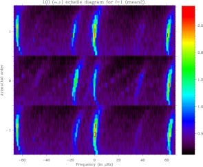
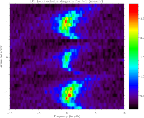
Figure 2: $(m,\nu)$ echelle diagramme for 1 year of LOI data for $l=1$. The scale is in ppm $\mu$Hz^-1/2. The spacing is tuned for $l=1$. (Left) The full diagramme centered on $l=1$. The $l=3$ modes are located about 15 $\mu$Hz at the left hand side of the $l=1$. The $l=2$ modes are on the right edge, while the $l=0$ are on the opposite side. The $l=4$ modes can be seen around +40 $\mu$Hz. (Right) The same diagramme but enlarged around $l=1$. The frequency shift or splitting of the modes due to the solar rotation can be seen: the 2 patches of power for $m=-1$ and $m=+1$ are slightly displaced from each other. The artificial correlation between $m=-1$ and $m=+1$ is not as clear.

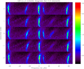
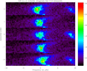
Figure 3: $(m,\nu)$ echelle diagramme for 1 year of LOI data for $l=2$. The scale is in ppm $\mu$Hz^-1/2. The spacing is tuned for $l=2$. (Left) The full diagramme centered on $l=2$ with a spacing of 135. $\mu$Hz. The $l=0$ modes are located about 10 $\mu$Hz at the right hand side of the $l=2$ modes. The $l=3$ modes are on the right edge, while the $l=1$ modes are on the opposite side. The $l=4$ modes are easily seen at about -25 $\mu$Hz; the $l=5$ starts to appear at +25 $\mu$Hz. (Right) The same diagramme but enlarged around $l=2$ with the $l=0$ modes at the right hand side. The splitting of the modes is clear. Note the absence of the $l=0$ modes for $m=\pm 1$

Figure 4: $(m,\nu)$ echelle diagramme for 1 year of LOI data for $l=5$. The scale is in ppm $\mu$Hz^-1/2. The spacing is tuned for $l=5$. Here we can clearly see the splitting of the $l=5$ modes. Unfortunately, the $l=5$ data of the LOI are heavily polluted by the presence of the $l=8$ modes. But since the spacing for the $l=8$ modes is different compared with that of the $l=5$ modes, the $l=8$ modes are seen as ridges going from lower left to upper right in each $m$ panel; while the $l=5$ modes are seen more like straight ridges in each $m$ panel. It can also be seen that the $|m|=5$ Fourier spectra contain information both about $m=\pm 5$. This is the result of the large LOI pixel size creating oversampling. The $l=8$ modes are also distinguished because the ‘splitting’ of this alias is in the opposite direction compared with that of the $l=5$ modes.

3 Application to data

3.1 ($m,\nu$) echelle diagramme for the LOI/SOHO data

Example of these diagrammes can be seen in Figs. 2, 3 and 4 for 1 year of LOI data for $l=1,2$ and 5, respectively. It is important when one makes such diagrammes to tune the spacing for the degree to study. For example, one can see in Fig. 2 that the ridges of power of $l=0,1,2$ and 3 have different shapes than in Fig. 3. Other modes with a significant different spacing can be seen more like diagonal ridges crossing the $(m,\nu)$ diagrammes; this is a powerful tool to identify other degrees. In Fig. 4, the $l=5$ $(m,\nu)$ echelle diagramme is clearly contaminated by an other degree, i.e. $l=8$, which appears at different frequencies depending on $m$. For $l=5,m=-5$, the $l=8,m=+8$ is quite strong; while for $l=5,m=+5$, this is $l=8,m=-8$ which shows up. This kind of ‘anti’-splitting behaviour is typical of any aliasing degrees. It is more prominent in the LOI data because of the undersampling effect due to the large size of the LOI pixels.

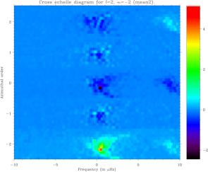
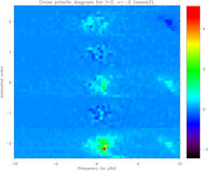
Figure 5: Effect of a wrong sign on the cross echelle diagrammes for 1 year of LOI data for $l=2,m=-2$. The scale is in ppm² $\mu$Hz^-1. The spacing is tuned for $l=2$. (Left) For the real parts or $\mbox{Re}(y_{l,m}(\nu))\mbox{Re}(y_{l,m^{\prime}}(\nu))$. (Right) For the imaginary parts or $\mbox{Im}(y_{l,m}(\nu))\mbox{Im}(y_{l,m^{\prime}}(\nu))$ without having the sign corrected. The real part of the cross echelle diagramme is constructed by the sum of those 2 quantities; compensation due to different signs will be misleading. The correlation of the real parts will always have the correct sign. This can be used for checking that the correlation of the imaginary parts for $m=0$ and $m=2$ is different from that of the correlation of the real parts.

Table 1: Theoretical leakage matrix of $l$=5 for the LOI data.

							$m^{\prime}$
		-5	-4	-3	-2	-1	0	1	2	3	4	5
	-5	1	0	0.18	0	-0.10	0	0.08	0	0.19	0	-0.45
	-4	0	1	0	0.27	0	-0.13	0	0.17	0	0.03	0
	-3	0.18	0	1	0	0.64	0	-0.21	0	-0.62	0	0.19
	-2	0	0.27	0	1	0	0.50	0	-0.18	0	0.17	0
	-1	-0.10	0	0.64	0	1	0	0.52	0	-0.21	0	0.08
$m$	0	0	-0.13	0	0.50	0	1	0	0.50	0	-0.13	0
	1	0.08	0	-0.21	0	0.52	0	1	0	0.64	0	-0.10
	2	0	0.17	0	-0.18	0	0.50	0	1	0	0.27	0
	3	0.19	0	-0.62	0	-0.21	0	0.64	0	1	0	0.18
	4	0	0.03	0	0.17	0	-0.13	0	0.27	0	1	0
	5	-0.45	0	0.19	0	0.08	0	-0.10	0	0.18	0	1

3.2 A useful detail

Before using the other diagrammes on real data, we need to point out a very important property coming from the way the $m$ signals are built. If the weights $W_{l,m}$ applied to the images, to extract an $l,m$ mode, have the same properties as of the spherical harmonics then we have:

$$W_{l,m}=W_{l,-m}^{*}$$ (10)

which means that both the Fourier spectra of $+m$ and $-m$ can be obtained from using a single filter $W_{l,+m}$. The Fourier spectrum of $+m$ will be in the positive part of the frequency range, while that of $-m$ will be in the negative part. This approach was first used by Rhodes et al. (1979) for measuring solar rotation, and mentioned theoretically by Appourchaux and Andersen (1990) for the case of the LOI. Due to the property of the Fourier transform, we recover, in the negative part of the frequency range, not the Fourier spectrum of $-m$ but its conjugate. This fact is very important, if one does not take care of the sign of the imaginary part of $-m$, it will lead to very serious problem. Needless to say that fitting data without taking into account this detail will have devastating effects. Figure 5 shows 2 cross echelle diagrammes for the real and imaginary parts of the spectra of $l=2$; the latter part had no sign compensation for $m<0$. Obviously this important detail cannot be detected in the power spectra.

3.3 Leakage matrix measurement for a single degree

3.3.1 LOI/SOHO data

According to theoretical computation of the p-mode sensitivities of the LOI pixels (Appourchaux and Andersen, 1990) and using the real shape of the LOI pixels (Appourchaux and Telljohann, 1996), the leakage matrices of $l=1$ and 2 are given by:

$$\@tens{\cal{C}}^{(1,1)}=\left(\begin{array}[]{ccc}1&0&\alpha\\ 0&1&0\\ \alpha&0&1\\ \end{array}\right)$$ (14)

$$\@tens{\cal{C}}^{(2,2)}=\left(\begin{array}[]{ccccc}1&0&\alpha_{1}&0&\alpha_{4}\\ 0&1&0&\alpha_{2}&0\\ \alpha_{3}&0&1&0&\alpha_{3}\\ 0&\alpha_{2}&0&1&0\\ \alpha_{4}&0&\alpha_{1}&0&1\\ \end{array}\right)$$ (20)

with: $\alpha=0.474$, $\alpha_{1}=\alpha_{3}=-0.308$, $\alpha_{2}=0.576$, $\alpha_{4}=-0.216$. The leakage matrix of $l=5$ is given in Table 1. These leakage matrices are mean value over one year. The leakages vary throughout the year because the distance between SOHO and the Sun varies. There is no $B$ angle effect as the mean $B$ is zero over 1 year. All the leakage elements are real as the LOI filters have the same symmetry as the spherical harmonics.

Figure 6, 7 and 8 display the cross echelle diagramme for $l=1,2$ and 5, respectively. From Figs. 6 and 7, we can directly verify using Eq. (6) the sign, and sometimes even the magnitude of the leakage elements. The best cross check that our theoretical computations are correct is to apply the inverse of the leakage matrices to the original data (See Section 2.2). Figures 9 and 10 show how the artificial correlations (or $m$ leaks) can be removed from the LOI data; for the latter we also cleaned the original data from the presence of the $l=0$ modes. We shall see later on with the GONG data that cleaning, similar to that of the LOI, can be achieved not only for 2 degrees but also for 3 degrees ($l=1,6$ and 9).

Unfortunately, the leakage matrix of $l=5$ for the LOI data cannot be inverted. This is the result of the pixel undersampling and has two dramatic consequences: the leakage matrix cannot be verified as for the $l=2$, and fitting the data as described in Part I is not valid anymore as the leakage matrix needs to be invertible. It means that the $2l+1$ Fourier spectra of $l=5$ are dependent. One way around the problem is to restrict the fitting to truly independent Fourier spectra. This problem is specific to the LOI data and applies only for $l\geq 4$.

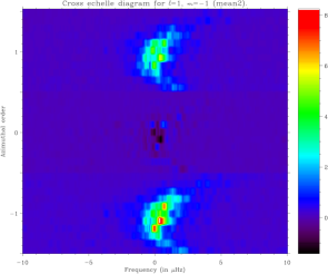
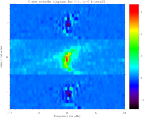
Figure 6: Real part of the cross echelle diagrammes for 1 year of LOI data for $l=1$. The scale is in ppm² $\mu$Hz^-1. The spacing is tuned for $l=1$. (Left) For $l=1,m=-1$. The lower panel represents the echelle diagramme of $m=-1$. The 2 other panels are the cross spectra with $m=0$ and $m=1$. As predicted, there is no visible correlation between $m=-1$ and $m=0$ while there is between $m=-1$ and $m=+1$. Here we visualize the first line of the real part of the matrix $\@tens{\cal{V}}^{(1,1)}$. (Right) For $l=1,m=0$. The bottom panel is the same as the middle panel of the left diagramme but with a different color scale. The middle panel is the power spectra of $m=0$ already shown in Fig. 2; the $l=6$ modes are visible as a diagonal ridge crossing the ridge of the $l=1$ modes.

Figure 7: Real part of the cross echelle diagrammes for 1 year of LOI data for $l=2$. The scale is in ppm² $\mu$Hz^-1. The spacing is tuned for $l=2$. (Top, left) For $m=-2$. The middle panel (for $m^{\prime}=0$) has negative ‘power’ close to the frequencies of the $m=-2$, indicating that $\alpha_{3}$ is negative. There is some indication that $\alpha_{1}$ may be negative. The upper panel (for $m^{\prime}=2$) has 2 patches of negative ‘power’ close to the frequencies of $m=-2$ and $m=+2$, showing that $\alpha_{4}$ is also negative. These 2 patches are clearly separated because of the mode splitting. (Top, right) For $m=-1$. Here it is obvious that $\alpha_{2}$ is positive. (Opposite) For $m=0$. There is now 2 patches of negative power in 2 opposite panels ($m^{\prime}=-2$ and $m^{\prime}=2$) due to the negativity of $\alpha_{3}$. It is likely that $\alpha_{1}$ is also negative.

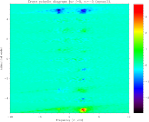
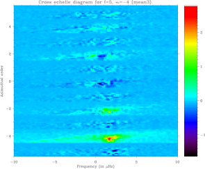
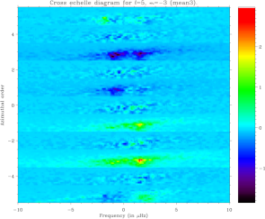
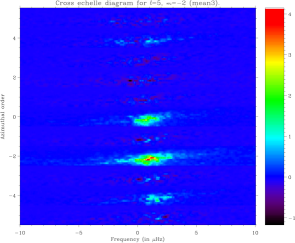
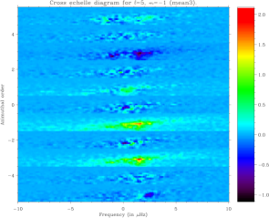
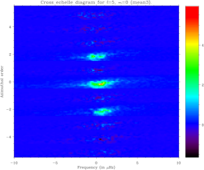
Figure 8: Real part of the cross echelle diagrammes for 1 year of LOI data for $l=5$. The scale is in ppm² $\mu$Hz^-1. The spacing is tuned for $l=5$. (Top, left) For $m=-5$. Here we can see the strong leakage of $m^{\prime}=5$ into $m=5$ and vice versa. The 2 patches of negative ‘power’ on the upper panel (or positive on the lower panel) are the $m=\pm 5$ modes separated by about 4-5 $\mu$Hz. (Top, right) For $m=-4$. Leakages between $m=-4$ and $m=-2$ are visible, but weaker than for $m=-5$. (Middle, left) For $m=-3$. Strong leakages between $m=-3$ and $m=+3$. (Middle, right) For $m=-2$. (Bottom, left) For $m=-1$. (Bottom, right) For $m=0$. The left diagrammes show more leakages compared with the right ones, the $l+m$ parity makes the difference.

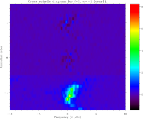
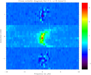
Figure 9: Real part of the cross echelle diagrammes of 1 year of LOI data for $l=1$. The scale is in ppm²$\mu$Hz^-1. The inverse of the theoretical leakage matrix has been applied to the original data with $\alpha$=0.474. (Left) For $l=1,m=-1$. The artificial correlation between $m=-1$ and $m=+1$ has been entirely removed (See Fig. 6 for comparison). (Right) For $l=1,m=0$. There is no improvement as there was no correlation before.

Figure 10: Real part of the cross echelle diagrammes of 1 year of LOI data for $l=2$ after having applied the inverse of the leakage matrix. The scale is in ppm² $\mu$Hz^-1. The spacing is tuned for $l=2$. (Top, left) For $m=-2$. (Top, right) For $m=-1$. (Opposite) For $m=0$. Using the inverse of the leakage matrix we have removed all artificial correlations (See Fig. 7 for comparison). The spectra have been cleaned both from the $m$ leaks and from $l=0$ modes because we used the leakage matrix of $l=2$ and $l=0$.

3.3.2 GONG data

The leakage matrices of the GONG data have been computed by R.Howe (1996, private communication). We also computed similar leakage matrices using the equations developed in Part I. The integration was made in the $\theta,\phi$ plane with $\theta_{max}=65.2^{\circ},\phi_{max}=53.5^{\circ}$ without apodization. We also took into account the effect of subtracting the velocity of the Sun seen as a star which affects GONG instrument’s sensitivity to modes only detected by integrated sunlight instrument (mainly the modes for which $l+m$ is even). The theoretical leakage matrices of $l=1$ and 2 for GONG are also given by Eq. (20) but with: $\alpha=-0.55$, $\alpha_{1}=-0.268$, $\alpha_{2}=0.451$, $\alpha_{3}=-0.122$, and $\alpha_{4}=-0.290$. For $l=1$, the leakage between $m=-1$ and $m=+1$ is negative due to the subtraction of the mean velocity which affects these modes. For $l=2$, the leakage between $m=-1$ and $m=+1$ has about the same value as for the LOI; these modes are not affected by the subtraction.

The cross echelle diagrammes of the $l=2$ GONG data are very close to those of the LOI (See Fig. 7). Figure 11 shows an example of a GONG cross echelle diagramme after having applied the inverse of the leakage matrix. It is clear that the p-mode correlations are removed. For $l=1$ we have used the cross echelle diagramme of $m=-1$ and $m=1$ for inferring quantitatively the off-diagonal leakage element $\alpha$. We first applied the inverse of a leakage matrix to the $l=1$ data, and then constructed the cross echelle diagramme of $m=-1$ and $m^{\prime}=1$ for these data. We then collapsed this diagramme by adding up all the modes with $n=10-26$, and finally we corrected the collapsed diagramme from the solar noise background. The collapsed diagramme is shown in Fig. 12 (Left) for no correction ($\alpha=0$) and for an $\alpha$ of -0.53; the corrected surface of the collapsed diagramme as a function of $\alpha$ is shown on Fig. 12 (Right). When the corrected surface is close to 0, there is no artificial correlation remaining.

Cleaning the data from artificial correlations has also been done in a different way by Toutain et al. (1998). Using Singular Value Decomposition, they recomputed pixel filters for the MDI/LOI proxy so as to remove the $m$ leaks and the other aliasing degrees. Here we have shown, that data cleaning is also possible without having the pixel time series, but using the Fourier spectra. This latter cleaning technique is more useful as one has to reduce a smaller amount of data.

Figure 11: Real part of the cross echelle diagrammes for 360 days of GONG data for $l=2$ after having applied the inverse of the leakage matrix. The scale is in m${}^{2}\,$s${}^{-2}\,$Hz^-1. The spacing is tuned for $l=2$. (Top, left) For $m=-2$. (Top, right) For $m=-1$. (Opposite) For $m=0$. As for the LOI data the artificial correlations are removed.

Figure 12: (Left) Collapsed diagramme of the real part of the cross spectrum of $m=-1$ and $m=+1$ for the GONG data after having applied the inverse of the leakage matrix, (top) no correction, (bottom) $\alpha$=-0.53. (Right) Surface of the collapsed diagramme as a function of $\alpha$, the surface is 0 for $\alpha$=-0.53.

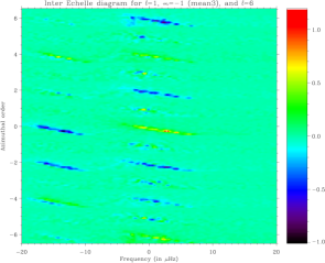
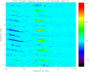
Figure 13: Real part of the inter echelle diagrammes for 1 year of LOI data for $l=1$ and $l^{\prime}=6$. The scale is in ppm² $\mu$Hz^-1. The spacing is tuned for $l^{\prime}=6$. (Left) For $l=1,m=-1$. Given the structure of the ridges, it means that the $l=1$ modes leak into the even $m$ modes of $l^{\prime}=6$, while the $l^{\prime}=6$ modes do not leak into the $l=1$. (Right) For $l=1,m=0$. Again using the structure of the ridges, the odd $m^{\prime}$ of $l^{\prime}=6$ leaks weakly into $l=1,m=0$.

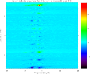
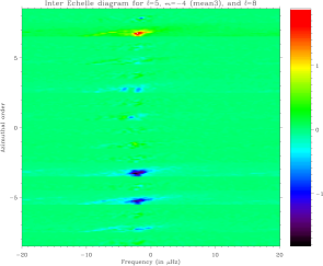
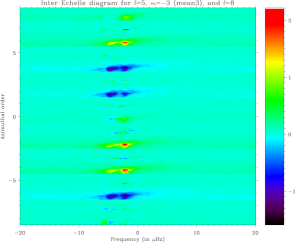
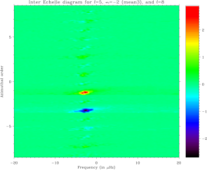
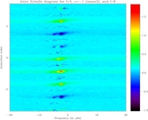
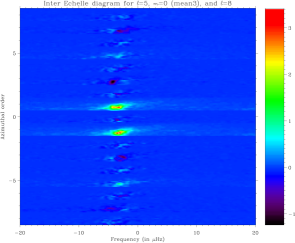
Figure 14: Real part of the inter echelle diagrammes for 1 year of LOI data for $l=5$ and $l^{\prime}=8$. The scale is in ppm² $\mu$Hz^-1. The spacing is tuned for $l^{\prime}=5$. (Top, left) For $l=5,m=-5$. (Top, right) For $l=5,m=-4$. (Middle, left) For $l=5,m=-3$. (Middle, right) For $l=5,m=-2$. (Bottom, left) For $l=5,m=-1$. (Bottom, right) For $l=5,m=0$. The $l=5$ ridges are more like vertical lines while those of the $l=8$ are more like diagonal lines going across from left to right.

3.4 Leakage matrix measurement for many degrees

3.4.1 LOI/SOHO data

Figures 13 and 14 shows the inter echelle diagramme for $l=1$, $l^{\prime}=6$, and $l=5$, $l^{\prime}=8$, respectively. These diagrammes are more difficult to interpret, but using specific spacing for $l$ or $l^{\prime}$, one can unambiguously identify which degree contributes to the correlation. For the LOI data, the $l=5$ and $l=8$ (similarly $l=4$ and $l=7$) are contaminated by each other. This is again due to the spatial undersampling which prevents the LOI data to be cleaned from aliasing degrees making the leakage matrix not invertible. Fortunately, the $l=1$ LOI data are far less affected by the presence of $l=6$ compared with that of GONG (See in the next section); this is the result of an effective apodization function (limb darkening) which creates a narrower spatial response than that of GONG (line-of-sight projection).

Figure 10 has already shown that we could clean the $l=2$ LOI data from the $l=0$ mode. This was done by taking into account the leakage matrix $\@tens{\cal{C}}^{(0,2)}$. Unfortunately as mentioned for the $l=5$, the LOI data cannot be cleaned from aliasing degrees because the leakage matrice $\@tens{\cal{C}}^{(1,6)}$, $\@tens{\cal{C}}^{(4,7)}$ and $\@tens{\cal{C}}^{(5,8)}$ are singular.

3.4.2 GONG data

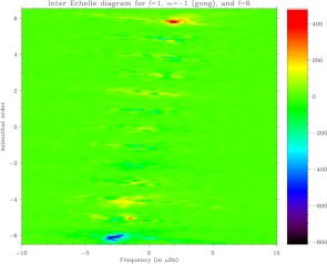
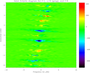
Figure 15: Real part of the inter echelle diagrammes of 1 year of GONG data for $l=1$ and $l^{\prime}=6$. The scale is in m${}^{2}\,$s${}^{-2}\,$Hz^-1. The spacing is tuned for $l^{\prime}=6$. (Left) For $l=1,m=-1$. The strongest correlations are for $m^{\prime}=\pm 6$ due to $l^{\prime}=6$. (Right) For $l=1,m=0$. The $l=6$ modes are strong in all the panels. For $m^{\prime}=\pm 1$ other modes can be seen as an ‘asterisk’ ridge: the ridge going from bottom right to upper left represents the $l=1$ modes; the ridge going from bottom left to upper right represents the $l=9$ modes; the vertical ridge represents the $l=6$ modes. At the far left, the ridge parallel to that of the $l=1$ represents the $l=3$ modes.

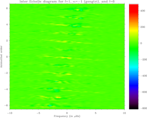
Figure 16: Real part of the inter echelle diagrammes of 1 year of GONG data for $l=1$ and $l^{\prime}=6$ after having applied the inverse of the leakage matrix $\@tens{\cal{C}}^{(1,6,9)}$. The scale is in m${}^{2}\,$s${}^{-2}\,$Hz^-1. The spacing is tuned for $l^{\prime}=6$. (Left) For $l=1,m=-1$. The faint yellow oblique ridges are due to the $l=1$ modes. (Right) For $l=1,m=0$. The correlations due to the $l=1$ and 6 modes are almost entirely removed.

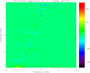
Figure 17: Real part of the inter echelle diagrammes of 1 year of GONG data for $l=1$ and $l^{\prime}=9$. The scale is in cm² s${}^{-2}\,\mu$Hz^-1. The spacing is tuned for $l=9$. (Left) For $l=1,m=-1$. The strongest correlations are for $m^{\prime}=\pm 9$ due to the $l^{\prime}=9$ modes. (Right) For $l=1,m=0$. The strongest correlations are for $m^{\prime}=0,\pm 1$ mainly due to the $l^{\prime}=9$ modes. A faint oblique ridge can be seen for $m^{\prime}=0$ due to the $l=1$ modes.

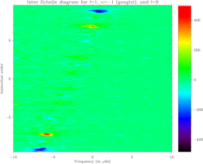
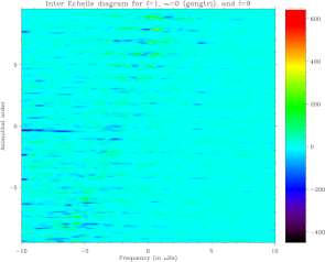
Figure 18: Real part of the inter echelle diagrammes of 1 year of GONG data for $l=1$ and $l^{\prime}=9$ after having applied the inverse of the leakage matrix $\@tens{\cal{C}}^{(1,6,9)}$. The scale is in cm² s${}^{-2}\,\mu$Hz^-1. The spacing is tuned for $l^{\prime}=9$. (Left) For $l=1,m=-1$. The correlations due $l=9$ are not correctly compensated for. (Right) For $l=1,m=0$. The $l=3$ correlation are also enhanced; they can be seen as oblique ridges at the left hand side of the diagrammes.

Figures 15 and 17 show the inter echelle diagramme for $l=1,l^{\prime}=6$, and for $l=1,l^{\prime}=9$. The correlations are clearly visible. If they are not taken into account they are likely to bias the frequency and splittings of the $l=1$ (See Rabello-Soares and Appourchaux, 1998, in preparation). By using the inverse full leakage matrix of $l=1,6$ and 9 (i.e. $\@tens{\cal{C}}^{(1,6,9)}$, one can clean the data from these spurious correlations arising both from the aliasing degrees and from the $m$ leaks. Figures 16 and 18 shows the ’cleaned’ inter echelle diagramme which should be compared with Figs. 15 and 17, respectively. The correlations have been almost entirely removed. Some correlations between the $l=1,m=-1$ modes and the $l=6,9$ modes are still present. This is due to the fact that the computation of the leakage for $l=1,m=\pm 1$ are very sensitive to the subtraction of the velocity of the Sun seen as a star. This is not the case for the $l=1,m=0$ modes as they are insensitive to this effect. Nevertheless, our imperfect knowledge of the leakage matrix can be adjusted in order to remove the residual correlations. It helped to reduce the systematic errors of the $l=1$ splitting at high frequencies, mainly where the $l=6$ start to cross over the $l=1$ (Rabello-Soares and Appourchaux 1998, in preparation).

It is possible to apply this cleaning technique to higher degree modes ($l\approx 50-100$. In principle, this is feasible, although the plethora of data involved may be fairly substantial. For higher degrees, the ridges of the modes in the $(m,\nu)$ echelle diagrammes are almost parallel to each other. The idea would be not to use the full Fourier spectra, as we did for the low degree GONG data, but to use only a small frequency range of about $\pm$ 30 $\mu$Hz around the target degree. By doing so, we will not only clean the data from the aliasing degrees but also from the $m$ leaks. In this case, the mode covariance matrix is diagonal. If we assume, wrongly, that the noise covariance matrix is diagonal, the statistics of each cleaned spectrum, for high degree modes, could be approximated by a $\chi^{2}$ with 2 degree of freedom. Neglecting the off-diagonal elements of the noise covariance matrix will lead to larger mode linewidth, thereby producing underestimated splittings; this systematic bias will decrease as the degree. This approximation will produce much less systematic errors than the approximation used by Hill et al. (1996) for the original data. The use of the suggested approximation for the GONG data may help, at the same time, to reduce systematic errors, and to increase computing speed for higher degree modes. The degree where one needs to switch between this approximation and the correct analysis needs to be determined.

3.5 Noise covariance matrix measurement

3.5.1 LOI/SOHO data

The leakage and ratio matrices have similar properties (See Part I). For example, for a given $l$ there is no correlation between the $m$ for which $m+m^{\prime}$ is odd for either matrix. This lack of correlation can be seen in Fig. 19 for the ratio cross spectra of the LOI data. The ratio matrix is also useful if one wants to reduce the number of noise parameters to be fitted. This is useful when the noise background, mainly of solar origin, varies slowly over the p-mode range. In this case the ratio can be assumed to be constant over the p-mode range. For example for $l=1$ we can fit 2 noise parameters instead of 3. When the noise varies in the p-mode range, it is more advisable to fit as many noise parameters as required.

Figure 20 shows the ratio cross spectra of $l=2$ for the LOI data. As this is commonly the case for the LOI, the ratios are independent of frequency. In addition, as outlined in Part I, the ratio matrix is very close to the leakage matrix. Using the values of $\alpha$ given for the LOI in Eq. (20) and Fig. 20, one can see that this is the case for the LOI. The ratio matrix has even the same symmetry property as the leakage matrix. In the case of the LOI, we sometimes use the independence of the ratio with frequency to reduce the number of free parameters. It is less straightforward to measure the noise correlation for the GONG data than for the LOI data. We recommend to measure it in between the p modes because that is what the fitting routines will determine.

3.5.2 GONG data

Figures 21 and 22 show the ratio cross spectra of $l=2$ for the GONG data. The ratio matrices (as the leakage matrices) are not symmetrical. Apart from the $l=1$, these matrices tend to be very close to those of the leakage matrices (see previous section). It is also clear that the ratios depend upon frequency, probably due to the effect of mesogranulation affecting the spatial properties of the noise with frequency. In this case, we cannot reduce the number of parameters to be fitted (see Rabello-Soares and Appourchaux 1998, in preparation) as we do for the LOI.

4 Summary and Conclusion

For helping the understanding of fitting p-mode Fourier spectra, we have devised 4 new helioseismic diagnostics:

1. the $(m,\nu)$ echelle diagramme helps visualizing:

   • which degree can be detected,

   • the mode splitting and

   • spurious degrees.

2. the cross echelle diagramme helps verifying:

   • the sign of the imaginary parts of the Fourier spectra for $m<0$,

   • the sign of the elements of the leakage matrix of the degree $l$,

   • to the first order the theoretical leakage matrix of the degree $l$ by applying the inverse of this matrix to the data (i.e. cleaning the data from the $m$ leaks) and

   • the cleaning of the data from $m$ leaks.

3. the inter echelle diagramme helps verifying:

   • the sign of the elements of the full leakage matrix for degrees $l,l^{\prime}$,

   • to the first order the theoretical leakage matrix of the degree $l,l^{\prime}$ by applying the inverse this matrix to the data and

   • the cleaning of the data from aliasing degrees.

4. the ratio cross spectrum helps deriving :

   • the amplitude of the noise correlation between the Fourier spectra and

   • the frequency dependence of the correlations.

These steps will help to evaluate the matrices of the leakage, mode covariance, ratio and noise covariance directly from observations. The fitting of the p modes will be considerably eased by verifying that the theoretical knowledge of these matrices is correct.

These steps have been used both on data for which we design the spatial filtering (LOI instrument), and on data for which we did not design the filtering (GONG). As a matter of fact these diagnostics are so powerful that a theoretical knowledge of the various matrices is not always necessary to understand the data. Very often these diagnostics can also be used to find bugs in the data analysis routines (Fig. 5). Nevertheless, it is advisable to know to the first order the leakage and ratio matrices for speeding up the analysis process.

Last but not least, the knowledge of the leakage matrices can be used for cleaning the data from $m$ leaks and from undesired aliasing degrees. This cleaning can be performed either when the pixel time series are available (MDI data, Toutain et al. , 1998) or more simply when only the Fourier spectra are available (LOI, GONG). The cleaning has very useful application for the GONG velocity data for removing aliasing degrees from $l=1$, 6 and 9 for instance, and for inferring better $l=1$ splittings (Rabello-Soares and Appourchaux 1998, in preparation). The cleaning is somewhat easier with Fourier spectra as one does not need to reduce large amount of image time series. It is advisable that, in the near future, this cleaning technique be used for higher degree modes. This will hopefully provide helioseismology with frequency and splitting data having much less systematic errors than before.

Figure 19: Real part of the ratio cross spectra for $l=1$. (Left) For $m=-1$ and $m^{\prime}$=0. There is very little correlation, less than -0.05. The modes also are not seen. (Right) For $m=-1$ and $m=1$. The noise correlation is about 0.55. The modes are visible with various positive and negative correlation.

Figure 20: Real part of the ratio cross spectra of $l=2$ for the LOI data. (Top, left) For $m=-2$ and $m^{\prime}=0$. The noise correlation is about -0.45. (Top, right) For $m=-2$ and $m=2$. The noise correlation is about -0.20. (Bottom, left) For $m=-1$ and $m^{\prime}=1$. The noise correlation is about 0.60. (Bottom, right) For $m=0$ and $m^{\prime}=2$. The noise correlation is about -0.35 same as for $m=-2$ and $m^{\prime}=0$.

Figure 21: Real part of the ratio cross spectra of $l=1$ for the GONG data. (Left) For $m=-1$ and $m^{\prime}$=0. As for the LOI, there is very little correlation, less than -0.05. The modes also are not seen. (Right) For $m=-1$ and $m=1$. The noise correlation is -0.77. The correlation is negative because of the way the GONG data are reduced: the full-disk integrated velocity has been removed from the signal.

Figure 22: Real part of the ratio cross spectra of $l=2$ for the GONG data. (Top, left) For $m=-2$ and $m^{\prime}=0$. The noise correlation is rather small and about -0.1. (Top, right) For $m=-2$ and $m=2$. The noise correlation is frequency dependent, with a typical value at 3000 $\mu$Hz of about -0.3. (Bottom, left) For $m=-1$ and $m^{\prime}=1$. The typical value is 0.4. (Bottom, right) For $m=0$ and $m^{\prime}=2$. The typical value is -0.3

- (1) Appourchaux, T. and Andersen, B.N., 1990, Sol.Phys. 128, 91
- (2) Appourchaux, T. and Telljohann, 1996, LOI GSE and VDC specification Doc., Version 1.7, available on the VIRGO home page (ftp://ftp.estec.esa.nl/pub/loitenerife/virgo.html)
- (3) Appourchaux, T., Andersen, B.N., Fröhlich, Jiménez, A., Telljohann, U. and Wehrli, C., 1997, Sol. Phys., 170, 27
- (4) Brown, T., 1985, Nature, 317, 591
- (5) Grec, G., PhD thesis, Université de Nice, Nice
- (6) Hill, F., Stark, R.T., Stebbins, R.T. et al. , 1996, Science, 272, 1292
- (7) Rhodes, E.J., Deubner, F-L. and Ulrich, R.K., 1979, ApJ, 227, 629
- (8) Schou, J., 1992, PhD thesis, On the analysis of helioseismic data, Århus Universitet, Århus
- (9) Toutain, T., Kosovichev, A. and Appourchaux, T., 1998, IAU General assembly, Kyoto