Breaking the degeneracy between anisotropy and mass: The dark halo of the E0 galaxy NGC 6703

Abstract

We have measured line-of-sight velocity profiles (vps) in the E0 galaxy NGC 6703 out to $2.6R_{e}$. Comparing with the vps predicted from spherical distribution functions (dfs), we constrain the mass distribution and the anisotropy of the stellar orbits in this galaxy.

We have developed a non-parametric technique to determine the df $f(E,L^{2})$ directly from the kinematic data. We test this technique on Monte Carlo simulated data with the spatial extent, sampling, and error bars of the NGC 6703 data. We find that smooth underlying dfs can be recovered to an rms accuracy of $12\%$ inside three times the radius of the last kinematic data point, and the anisotropy parameter $\mathchar 28940\relax(r)$ to an accuracy of $0.1$, in a known potential. These uncertainties can be reduced with improved data.

By comparing such best-estimate, regularized models in different potentials, we can derive constraints on the mass distribution and anisotropy. Tests show that with presently available data, an asymptotically constant halo circular velocity $v_{0}$ can be determined with an accuracy of $\pm\mathrel{\hbox to0.0pt{\lower 3.0pt\hbox{$\mathchar 536\relax$}\hss}\raise 2.0pt\hbox{$\mathchar 316\relax$}}50{\rm\,km\,s^{-1}}$. This formal range often includes high–$v_{0}$ models with implausibly large gradients across the data boundary. However, even with extremely high quality data some uncertainty on the detailed shape of the underlying circular velocity curve remains.

In the case of NGC 6703 we thus determine the true circular velocity at $2.6R_{e}$ to be $250\pm 40{\rm\,km\,s^{-1}}$ at $95\%$ confidence, corresponding to a total mass in NGC 6703 inside $78^{\prime\prime}$ ($13.5\,h_{50}^{-1}{\rm\,kpc}$, where $h_{50}\equiv H_{0}/50{\rm km/s/Mpc}$) of $1.6-2.6\times 10^{11}h_{50}^{-1}{\rm\,M_{\odot}}$. No model without dark matter will fit the data; however, a maximum stellar mass model in which the luminous component provides nearly all the mass in the centre does. In such a model, the total luminous mass inside $78^{\prime\prime}$ is $9\times 10^{10}{\rm\,M_{\odot}}$ and the integrated B-band mass–to–light ratio out to this radius is $\Upsilon_{B}=5.3-10$, corresponding to a rise from the center by at least a factor of $1.6$.

The anisotropy of the stellar distribution function in NGC 6703 changes from near-isotropic at the centre to slightly radially anisotropic ($\mathchar 28940\relax\!=\!0.3-0.4$ at 30”, $\mathchar 28940\relax\!=\!0.2-0.4$ at 60”) and is not well-constrained at the outer edge of the data, where $\mathchar 28940\relax\!=\!-0.5-+0.4$, depending on variations of the potential in the allowed range.

Our results suggest that also elliptical galaxies begin to be dominated by dark matter at radii of $\sim 10{\rm\,kpc}$.

1 Introduction

Current cosmological models predict that, similar to spiral galaxies, elliptical galaxies should be surrounded by dark matter haloes. The observational evidence for dark matter in ellipticals is still weak, however. In a few cases masses have been determined from X-ray observations (e.g., Awaki et al. 1994, Kim & Fabbiano 1995) or HI ring velocities (Franx, van Gorkom & de Zeeuw 1994). In others it has been possible to rule out constant M/L from extended velocity dispersion data (Saglia et al. 1993), from absorption line profile measurements (Carollo et al. 1995, Rix et al. 1997), or from globular cluster or planetary nebula velocities (e.g., Grillmair et al. 1994, Arnaboldi et al. 1994). Gravitational lensing statistics (Maoz & Rix 1993) and individual image lens separations (Kochanek & Keeton 1997) favour models with extended dark matter haloes around ellipticals. Despite of this, the detailed radial mass distribution in elliptical galaxies remains largely unknown. Similarly, although we know from the tensor virial theorem that giant ellipticals are globally anisotropic (Binney 1978), their detailed anisotropy structure is only poorly known.

The origin of this uncertainty is a fundamental degeneracy – in general, it is impossible to disentangle the anisotropy in the velocity distribution and the gravitational potential from velocity dispersion and rotation measurements alone (Binney & Mamon 1982, Dejonghe & Merritt 1992). Tangential anisotropy, for example, can mimic the presence of dark matter. Recent dynamical studies have indicated, however, that the anisotropy of the stellar distribution function (df) is reflected in the shapes of the line-of-sight velocity profiles (vps) in a way that depends on the gravitational potential (Gerhard 1993, G93; Merritt 1993). These papers argued that the extra constraints derived from the vp measurements may be enough to break the degeneracy and determine the mass distribution.

If this is correct, it provides a new method to investigate the properties of the dark matter haloes around elliptical galaxies at intermediate radii: vps can now be estimated from high-quality absorption line measurements out to $\sim 3$ effective radii. Dynamical models are then used to disentangle the effects of orbital anisotropy and potential gradient on the vp shapes. In this paper, we implement these ideas for the analysis of real data, analyzing the E0 galaxy NGC 6703. This study is part of an observational and theoretical program aimed at understanding the mass distribution and orbital structure in elliptical galaxies. Preliminary accounts of this work have been given in Jeske et al. (1996) and Saglia et al. (1997a).

We have obtained long–slit spectroscopy for NGC 6703, and have measured vps to $\sim 2.6R_{e}$ with the method of Bender (1990). The results are quantified by a Gauss-Hermite decomposition (G93, van der Marel & Franx 1993) as described by Bender, Saglia & Gerhard (1994; BSG). These observations are described in Section 2. In Section 3 we use simple dynamical models to describe the variation of the vp shapes with anisotropy and potential, generalizing the results of G93 for scale–free models. These models, taken from a systematic study of the relation between df and vps in spherical potentials (Jeske 1995), are described in Appendix A. In Section 4 we develop a non-parametric method for inferring the df and potential from absorption line profile measurements. Tests on Monte Carlo generated data are used to determine the degree of confidence with which the df and potential can be inferred from real data. In Section 5 we analyse the kinematic data for NGC 6703. Comparison with the dynamical models from Jeske (1995) already shows that no constant–M/L model will fit the data. The non–parametric method developed in Section 4 is then used to derive quantitative constraints on the mass distribution and anisotropy of this galaxy. Finally, Section 6 presents a discussion of the results and our conclusions.

2 Observations of NGC 6703

NGC 6703 is an E0 galaxy at a distance $D\!=\!36$ Mpc (Faber et al. 1989) for $H_{0}\!=\!50$ km/s/Mpc. From a B-band CCD frame taken at the prime focus of the 3.5m telescope on Calar Alto and kindly provided by U. Hopp we have measured the inner surface brightness profile using the algorithm by Saglia et al. (1997b); this follows an $R^{1/4}$ law with $R_{e}\!=\!30^{\prime\prime}\!=\!5.2\,h_{50}^{-1}$ kpc, or a Jaffe model with $r_{J}\!=\!46.5^{\prime\prime}\!=\!8.1\,h_{50}^{-1}{\rm\,kpc}$, with small residuals (Fig. 1). A 3% increase of the sky value reduces the measured Jaffe radius to $35.5^{\prime\prime}$, a 1% decrease of the sky values increases it to $54^{\prime\prime}$. Isophote shapes deviate little from circles ($\mathchar 28943\relax\!<\!0.05$, $\mid a_{4}/a\mid<0.005$) and show small twisting ($\Delta PA\!\simeq\!10^{\circ}$). From the Jaffe profile fit we derive a fiducial (calibrated and corrected for galactic absorption following Faber et al. 1989) $M_{B}\!=\!-21.07$, or luminosity $L_{B}\!=\!4.16\times 10^{10}h_{50}^{-2}L_{\odot,B}$. Note that the values of $R_{e}$ and $M_{B}$ derived here are slightly larger than those ($R_{e}=24^{\prime\prime}$, $M_{B}=-20.79$) given by Faber et al. (1989).

The spectroscopic observations were carried out in October 1994, May 1995 and August 1995 with the 3.5-m telescope on Calar Alto, Spain. In all of the runs the same setup was adopted. The Boller & Chivens longslit twin spectrograph was used with a 1200 line mm^-1 grating giving 36 Å/mm dispersion. The detector was a Tektronix CCD with 1024$\times$1024 24$\mathchar 28950\relax$m pixels and the wavelength range 4760-5640 Å. The instrumental resolution obtained using a 3.6 arcsec wide slit was 85 km/s. We collected 1.5 hrs of observations along the major axis of the galaxy, 4 hrs of observations perpendicular to the major axis and shifted to the North-East of the center by 24 arcsec ($0.8R_{e}$), and 13 hours of observations perpendicular to the major axis and shifted to the North-East of the center by 36 arcsec ($1.2R_{e}$). Spectra taken parallel to the minor axis and shifted from the center allow at the same time a good sky subtraction and the symmetry check of the data points.

Figure 1: (a) Residuals of a Jaffe model fit to photometry for NGC 6703. Full line: in surface brightness; dotted line: in the curve of growth. The vertical dotted line marks the scaling Jaffe radius $r_{J}$. (b) Folded mean velocity, (c) velocity dispersion, (d) $h_{3}$, and (e) $h_{4}$ profiles. Crosses and filled circles refer to the two sides of the galaxy and the major axis spectrum. The small dots refer to the unrebinned spectrum (see text). Open and filled triangles refer to the two sides of the galaxy and the spectrum taken parallel to the minor axis and shifted 24 arcsec from the center. Open and filled squares refer to the two sides of the galaxy and the spectrum taken parallel to the minor axis and shifted 36 arcsec from the center.

The analysis of the data was carried out following the steps described by BSG. The logarithmic wavelength calibration was performed at a smaller step ($\Delta v=30$ km/s) than the actual pixel size ($\approx 50$ km/s) to exploit the full capabilities of the Fourier Correlation Quotient method. A sky subtraction better than 1% was achieved. The heliocentric velocity difference between the May 1995 and the September 1994 - August 1995 frames was taken into account before coadding the observed spectra. The spectra were rebinned along the spatial direction to obtain a nearly constant signal to noise ratio larger than 50 per resolution element. The effects of the continuum fitting and instrumental resolution were extensively tested by Monte Carlo simulations. The residual systematic effects on the values of the $h_{3}$ and $h_{4}$ parameters are expected to be less than 0.01. The resulting fitted values for the folded velocity $v$ , velocity dispersion $\mathchar 28955\relax$, $h_{3}$ and $h_{4}$ profiles are shown in Fig. 1 as a function of the distance from the center, reaching $\sim 2.6R_{e}$. The $v$ and $\mathchar 28955\relax$ profiles are folded antisymetrically with respect to the center for the major axis spectrum, symmetrically with respect to the major axis for the spectra parallel to the minor axis. Template mismatching was minimized by choosing the template star which gave the minimal symmetric $h_{3}$ profile derived along the major axis of the galaxy. The systematic effect due to the residual mismatching on the derived $h_{4}$ values estimated from the remaining symmetric components is less than 0.01.

The galaxy shows very little rotation ($\approx 0$ km/s for $R<R_{e}$, $\approx 20-30$ km/s for $R>R_{e}$). The (cylindrical) rotation measured parallel to the minor axis is slightly larger ($\approx 35$ km/s) along the 24 arcsec shifted spectrum, but consistent with the peak velocity reached along the major axis at $R\approx 22$ arcsec. This is shown by the velocities derived from the unbinned major axis spectra (dots in Fig. 1). The velocity dispersion drops from the central $\approx\!190$ km/s to $\approx\!140$ km/s at $R_{e}/2$, slowly declining to about 110 km/s in the outer parts. The $h_{3}$ and $h_{4}$ values are everywhere close to zero. The error bars are determined from Monte-Carlo simulations. Noise is added to template stars (rebinned to the original wavelength pixel size) broadened following the observed values of $\mathchar 28955\relax$ and $h_{4}$, matching the power spectrum noise to peak ratio of the galaxy spectra. The accuracy of the estimated error bars (the r.m.s. of 30 replica of the data points) is about 20 % (determined from the scatter of the estimated signal to noise ratios).

Data points at the largest distances for the different data sets have lower signal to noise ratio than the mean and therefore have larger error bars. In addition, these data points are expected to suffer more from the systematic effects due to the galaxy light contamination of the sky subtraction(see discussion in Saglia et al. 1993). They are in any case consistent within the error bars with the more accurate values derived from the other available spectra.

The observed scatter is sometimes slightly larger than expected from the error estimates. This excess could be real and due to the faint structures apparent in an unsharped mask image of the galaxy. In particular this applies to the asymmetries observed in the $h_{4}$ profile in the central 5 arcsec. The negative $h_{4}$ values detected for the first data points of the 24 arcsec shifted spectrum are also real. They are detected in the unbinned major axis spectra at $R\approx 22$ arcsec (dots in Fig. 1).

Figure 2: Fitted projected velocity dispersion $\mathchar 28955\relax_{\rm fit}$, anisotropy parameter $\mathchar 28940\relax$, and vp-parameter $h_{4}$ for representative Jaffe models in self-consistent (left) and halo potential (right). The models shown are radially and tangentially anisotropic models constructed with the method of G91 (dashed lines), the isotropic model (solid), and two Osipkov-Merritt models (dotted lines). Note that while $\mathchar 28940\relax$ is a function of three-dimensional radius $r$ and $\mathchar 28955\relax_{\rm fit}$, $h_{4}$ are observed quantities depending on projected radius $R$, there is a close correspondence between features in these profiles. See text.

3 Velocity profiles in spherical galaxies

To better understand the relation between vp–shape, anisotropy, and gravitational potential, we have constructed a large number of anisotropic models for spherical galaxies in which the stars follow a Jaffe (1983) profile. The gravitational potential was taken to be either that of the stars (self-consistent case), or one with everywhere constant rotation speed (‘halo potential’). The latter case corresponds to a mass distribution with a dark halo which has equal density as the stars at $r\!\simeq\!0.4r_{J}$, and equal interior mass at $r\!\simeq\!r_{J}$, where $r_{J}$ is the scale radius of the Jaffe model. Anisotropic quasi-separable distribution functions (dfs) $g(E)\,h(E,L^{2})$ were calculated by the method of Gerhard (1991; G91), but contrary to G93 the circularity function (which specifies the distribution of angular momenta on energy shells) was allowed to vary with energy. These models include dfs in which the anisotropy changes radially, from tangential to radial or vice-versa, from isotropic to radial to tangential, etc. (see Fig. 18). For comparison, we have also constructed families of Osipkov (1979) - Merritt (1985) models which become strongly radially anisotropic beyond a certain radius. Details of this model data base and the properties of their vps are given in Appendix A and in Jeske (1995); here we only give a brief summary relevant for the comparison with NGC 6703.

The shapes of the observable vps are most sensitive to the anisotropy of the df, but depend also on the potential (G93). For rapidly falling luminosity profiles, the vps are dominated by the stars at the tangent point. Then radially (tangentially) anisotropic dfs lead to more peaked (more flat-topped) vps than in the isotropic case; in terms of the Gauss-Hermite parameter $h_{4}$, this corresponds to $h_{4}\!>\!(h_{4})_{\rm iso}$ and $h_{4}\!<\!(h_{4})_{\rm iso}$, respectively (Figs. 8,9 in G93).

Fig. 2 shows that these trends are also seen in the present models in which both the luminosity density and the anisotropy change with radius. An increase in radial (tangential) anisotropy at intrinsic radius $r$ is accompanied by an increase (decrease) of $h_{4}$ at projected radius $R\!\simeq\!r$. The correspondence is strongest in the models’ outer parts, but is also seen to a lesser extent in the centre of a Jaffe model where $\mathchar 28954\relax(r)\propto r^{-2}$ – contrary to a homogeneous core where radial orbits lead to broadened vps (Dejonghe 1987). Quantitatively the correspondence depends also on the anisotropy gradient. Osipkov-Merritt-models show a reversal of this trend near their anisotropy radius $r_{a}$ due to the large number of high-energy radial orbits all turning around near $r_{a}$; this leads to flat-topped vps in a small radius range near $r_{a}$. However, the properties of these models are extreme and they are in general not very useful for modelling observed vps.

Fig. 2 and Figs. 8,9 in G93 also show that as the mass of the model at large $r$ is increased at constant anisotropy, both the projected dispersion and $h_{4}$ increase. Increasing $\mathchar 28940\relax$ at constant potential, on the other hand, lowers $\mathchar 28955\relax$ and increases $h_{4}$. This suggests that by modelling $\mathchar 28955\relax$ and $h_{4}$ both mass $M(r)$ and anisotropy $\mathchar 28940\relax(r)$ can in principle be found.

4 Modelling absorption line profile data

Having seen the effect of anisotropy and potential variations on the line profile parameters, we now proceed to construct an algorithm by which the distribution function and potential of a spherical galaxy can be constrained from its observed $\mathchar 28955\relax$ and $h_{4}$–profiles. Such absorption line profile data contain a subset of the information given by the projected distribution function $N({\ninebmi R},v_{\scriptscriptstyle\|})$, which in the spherical case is related to the full df by

$$N(R,v_{\scriptscriptstyle\|}) = \int\!dz\int\!\!\int\!dv_{x}dv_{y}f(E,L^{2})$$

$$= \int\!dz\int\!\!\int\!dv_{x}dv_{y}f[{\textstyle{1\over 2}}v_{r}^{2}+{\textstyle{1\over 2}}v_{t}^{2}+\Phi(r),r^{2}v_{t}^{2}].$$

Here the position on the sky is specified by ${\ninebmi R}=(x,y)$; $R=|{\ninebmi R}|$. Velocities in the sky plane are denoted by $(v_{x},v_{y})$, $z$ and $v_{\scriptscriptstyle\|}$ are the line-of-sight position and velocity, and $v_{r}$ and $v_{t}$ are the intrinsic radial and tangential velocities. In spherical symmetry, the df $f(E,L^{2})$ is a function of energy and squared angular momentum only.

Notice from eq. (1) that the projected df depends linearly on $f$, but non-linearly on the potential $\Phi(r)$. Thus $f$ will generally be easier to determine from $N(R,v_{\scriptscriptstyle\|})$ than $\Phi$. Moreover, while considerations like those in the last section do suggest that, in spherical symmetry and for positive $f(E,L^{2})$, both the df and the potential can be determined from $N(R,v_{\scriptscriptstyle\|})$, there is no theoretical proof that this is in fact true. We only know that in a fixed spherical potential the df is uniquely determined from $N(R,v_{\scriptscriptstyle\|})$ (Dejonghe & Merritt 1992). For these reasons we have found it useful to split our problem into two parts (see also Merritt 1993):

(1) We fix the potential $\Phi$, and from the photometric and kinematic data determine the “best” df $f$ for this potential. Because in practice the surface brightness (sb) profile is much better sampled than the kinematic observations and also has smaller errors, we treat it separately and determine the stellar luminosity density $j(r)$ at the beginning. The kinematic data are then used to determine the “best” $f$ for given $j(r)$ and $\Phi(r)$, by approximately solving equation (1) as a linear integral equation.

(2) We then vary $\Phi$ to find that potential which allows the best fit overall. At present, it is not practical in step (2) to attempt to determine the potential non-parametrically. Rather, we choose a parametrized form for $\Phi$, and find the region in parameter space for which the “best” df as determined in step (1) reproduces the data adequately.

In view of the modelling of NGC 6703 in Section 5, we have considered the following family of potentials, including a luminous and a dark matter component: The stellar component is approximated as a Jaffe (1983) sphere, with scale-radius $r_{J}$ and total mass $M_{J}$, so that

$$\Phi_{L}(r)={GM_{J}\over r_{J}}\ln{r\over r+r_{J}}.$$ (2)

The dark halo has an asymptotically flat rotation curve,

$$v_{c}(r)=v_{0}{r\over\sqrt{r^{2}+r_{c}^{2}}},$$ (3)

so that its potential is

$$\Phi_{H}(r)={\textstyle{1\over 2}}v_{0}^{2}\ln(r^{2}+r_{c}^{2}).$$ (4)

This is specified by the asymptotic circular velocity $v_{0}$ and the core radius $r_{c}$. Both the luminous and dark halo components can be modified when needed, and need not be analytic functions.

In testing our method below, we use parameters adapted to NGC 6703. This galaxy is well-fit by a Jaffe profile (Section 2), so $r_{J}$ is known. This leaves three free parameters, the mass $M_{J}$ or mass–to–light ratio $\Upsilon$ of the stellar component, and the halo parameters $r_{c}$ and $v_{0}$. If one assumes that the central kinematics is dominated by the luminous matter, $\Upsilon$ can be determined. Then only the two halo parameters $r_{c}$ and $v_{0}$ are free. The assumption of maximum stellar $\Upsilon$ is similar to the maximum disk assumption in spiral galaxies.

In any of the potentials specified by eqns. (2)–(4) we determine the df by the algorithm described in Section 4.1 below. To assess the significance of the results obtained, we test the algorithm on Monte Carlo–generated pseudo data in Section 4.2. For kinematic data with the spatial extent and observational errors such as measured for NGC 6703, the algorithm recovers a smooth spherical df $\sim 70\%$ of the time to an rms level of $\sim 12\%$, taken inside three times the radius of the outermost kinematic data point. In Section 4.3, we investigate the degree to which the gravitational potential can be constrained from similar data.

4.1 Recovering $f$ from $\mathchar 28955\relax$ and $h_{4}$, given $\Phi$

As discussed above, the projected distribution function $N(r,v_{\scriptscriptstyle\|})$ suffices to determine df $f(E,L^{2})$ uniquely. In practice, however, only incomplete and noisy data are available in place of $N(r,v_{\scriptscriptstyle\|})$, and contrary to the two-dimensional function $N(r,v_{\scriptscriptstyle\|})$, the observed $\mathchar 28955\relax(R_{i})$ and $h_{4}(R_{i})$ contain only one-dimensional information. This suggests that we can hope to recover only the gross features of $f$ from such kinematic data. Indeed, the anisotropy parameter $\mathchar 28940\relax(r)$ seems to be essentially fixed from accurate $h_{4}$ measurements (e.g., Figs. 8,9 in G93). Local fluctuations in the df will be inaccessible, but as we will show, smooth dfs can be recovered with reasonable accuracy from presently available data.

To solve the inversion problem, we first compute a set of self–consistent models $f_{k}(E,x)$ for the stellar density $j(r)$, in the fixed potential $\Phi(r)$. The $f_{k}(E,x)$ are models of the kind discussed in Section 2 and Appendix A; $E$ and $x$ are the energy and circularity integrals of the motion. Then we write the df as a sum over these “basis” functions:

$$f=\sum_{k=1,K}a_{k}f_{k}(E,x).$$ (5)

We do not need to use a doubly infinite, complete set of basis functions because most of the high–frequency structure represented by the higher–order basis functions in such a set will be swamped by noise in the observational data. It is sufficient to choose the number of basis functions, $K$, and the $f_{k}(E,x)$ themselves such that the data can be fitted with a mean $\mathchar 28959\relax^{2}\simeq 1$ per data point. We have found it advantageous to use the isotropic model plus tangentially anisotropic basis models, because with these the anisotropy of the final composite df (5) can be varied in a more local way than with radially anisotropic components. Since the $a_{k}$ can be negative, it is of course no problem to generate a radially anisotropic df from the isotropic model plus a set of tangential basis models.

Figure 3: Anisotropy parameter $\mathchar 28940\relax$ for a subset of basis functions $f_{k}$ used in the self–consistent Jaffe potential (top) and in a mixed Jaffe plus halo model (bottom). The top full line in each panel shows the isotropic model. All other basis models are tangentially anisotropic. Two values of asymptotic anisotropy as $r\rightarrow\infty$ are used (full and dashed lines). For illustration, the long–dashed lines show the $\mathchar 28940\relax$–profiles of the best–fitting dfs derived with these bases from the NGC 6703 data, in both potentials.

In Fig. 3 we illustrate the basis models we have used, by plotting radial profiles of the anisotropy parameter $\mathchar 28940\relax(r)$ for a subset of them. For these basis functions $\mathchar 28940\relax(r)$ can be regarded as a measure of the extent of the df in circularity $x$, at the energy $E=\Phi(r)$. The figure shows that the basis resolves three steps in $x$ in the limits $r\rightarrow 0$ and $r\rightarrow\infty$; at intermediate energies, it has much finer resolution. The majority of the number of functions is spent on resolving the energy dependence, i.e., on placing the main gradient zones of the functions $f_{k}$ in the ($E,x)$ plane on a relatively dense grid in energy. The main difference to using power law components (Fricke 1952, and, e.g., Dejonghe et al. 1996) is that our basis models are already reasonable in the sense that they are viable dynamical models for the density in question, and that the superposition is used only to match the kinematics. We have typically used $K\mathrel{\hbox to0.0pt{\lower 3.0pt\hbox{$\mathchar 536\relax$}\hss}\raise 2.0pt\hbox{$\mathchar 316\relax$}}20$ such functions; this proved sufficient even for analysing pseudo data of much better quality than we have for NGC 6703.

Each of the $f_{k}(E,x)$ reproduces the stellar density distribution $j(r)$; so the $a_{k}$ satisfy

$$\sum_{k=1,K}a_{k}=1.$$ (6)

Moreover, the coefficients $a_{k}$ must take values such that

$$\sum_{k=1,K}a_{k}f_{k}(E,x)\geq 0$$ (7)

everywhere in phase-space. In practice, these positivity constraints are imposed on a grid in energy and circularity $(E\!=\!E_{i},x\!=\!x_{j})$. Subject to these constraints the $a_{k}$ are to be determined such that the kinematics predicted from the df (5) match the observed kinematics in a minimum $\mathchar 28959\relax^{2}$–sense.

The comparison between model and data is not entirely straightforward, however. Since the measured ($v$, $\mathchar 28955\relax$, $h_{3}$, $h_{4}$) are obtained by fitting to the line profile (the observational analogue of the projected df), they unfortunately depend non-linearly on the galaxy’s underlying df. Thus we cannot use the observed $v$ and $\mathchar 28955\relax$ in a linear least squares algorithm to determine the $a_{k}$ from the data – they cannot be written as moments of $f$. In the fitting process, they have to be replaced by quantities that do depend linearly on the df. Moreover, the error bars for these new quantities generally depend not only on the observed error bars of $v$ and $\mathchar 28955\relax$, but also on the errors and the values of the line profile parameters $h_{3}$ and $h_{4}$. They must therefore be determined with some care.

We have investigated several schemes along these lines. The following seemed to do best in recovering a known underlying spherical df from pseudo data. From the measured ($\mathchar 28955\relax,h_{4}$), we compute an approximation to the true velocity dispersion (second moment) $\overline{\mathchar 28955\relax}^{2}(R_{i})$, by integrating over the line profile (for negative $h_{4}$, until it first becomes negative). We also evaluate a new set of even Gauss-Hermite moments $s_{n}(R_{i};\widetilde{\mathchar 28955\relax})$ from the data, using fixed, fiducial velocity scales $\widetilde{\mathchar 28955\relax}(R_{i})$ (G93, Appendix B). We have found it convenient to take for these $\widetilde{\mathchar 28955\relax}(R_{i})$ the velocity dispersions $\mathchar 28955\relax_{\rm iso}(R_{i})$ of the isotropic model with the galaxy’s stellar density, in the current potential $\Phi(r)$.

The velocity profile moments of the basis function models are transformed to the same velocity scales $\widetilde{\mathchar 28955\relax}(R_{i})$. The moments $\overline{\mathchar 28955\relax}^{2}(R_{i})$ and $s_{n}(R_{i};\widetilde{\mathchar 28955\relax})$ of the composite df then depend linearly on the corresponding moments of the basis function models. For a regularized model they are smooth functions of $R$, of which the (noisy) observational moments are assumed to be a random realisation within the respective errors.

To determine the best-fitting coefficient $a_{k}$ we minimize the sum over data points $i$ of all

$$\mathchar 28959\relax^{2}_{\mathchar 28955\relax,i}\equiv w^{2}_{\mathchar 28955\relax}(R_{i})\Big{[}\overline{\mathchar 28955\relax}^{2}(R_{i})-\sum_{k=1,K}a_{k}\overline{\mathchar 28955\relax}^{2}_{k}(R_{i})\Big{]}^{2}$$ (8)

and

$$\mathchar 28959\relax^{2}_{n,i}\equiv w^{2}_{n}(R_{i})\Big{[}s_{n}(R_{i};\widetilde{\mathchar 28955\relax})-\sum_{k=1,K}a_{k}s_{n}^{(k)}(R_{i};\widetilde{\mathchar 28955\relax})\Big{]}^{2}$$ (9)

for $n=2,4$. These equations make use of the fact that all the $f_{k}$ are self-consistent models for the same $j(r)$, so that all surface density factors $\mathchar 28950\relax_{k}(R_{i})\!=\!\mathchar 28950\relax(R_{i})$ cancel.

To determine the weights $w_{\mathchar 28955\relax}$ and $w_{n}$, we have done Monte Carlo simulations studying the propagation of the observational errors $\Delta\mathchar 28955\relax$ and $\Delta h_{4}$. Based on the results of these simulations, we have chosen

$$\immediate w_{\mathchar 28955\relax}^{-1}(R_{i}) = 2.4\overline{\mathchar 28955\relax}(R_{i})[\overline{\mathchar 28955\relax}(R_{i})/\mathchar 28955\relax(R_{i})]\Delta\mathchar 28955\relax(R_{i}),$$ (10)

$$\immediate w_{2}^{-1}(R_{i}) = 0.7\Delta\mathchar 28955\relax(R_{i})/\mathchar 28955\relax(R_{i}),$$ (11)

$$\immediate w_{4}^{-1}(R_{i}) = 0.95\mathchar 28939\relax\Delta h_{4}.$$ (12)

The coefficients are representative in the range of values taken by the observed error bars and the measured $h_{4}$. In the presently used fitting procedure, the additional dependence on $h_{4}$ and the respective “other” error bar is neglected – the tests below show that this leads to satisfactory results. Since to first order the $s_{2}$–moment thus measures the shift from $\mathchar 28955\relax$ to $\overline{\mathchar 28955\relax}$, the parameter $\mathchar 28939\relax$ in eq. (13) will be near $\mathchar 28939\relax\simeq 2$. We have fixed $\mathchar 28939\relax$ by requiring that the distributions of $\mathchar 28959\relax^{2}_{\mathchar 28955\relax}$ and $\mathchar 28959\relax^{2}_{h4}$ have equal width (see below); this results in $\mathchar 28939\relax=1.7$.

Finally, we assume that the df underlying the observed kinematics is smooth to the degree that is compatible with the measured data. Clearly, unless such an assumption is made, it is impossible to determine a function of two variables, $f(E,L^{2})$, from a small number of data points with real error bars. One way to ensure that the df is smooth is to use only a small number of terms in the expansion (5). However, this is not a good way of smoothing as it biases the recovered df towards the functional forms of the few $f_{k}$ that are used in the sum. A better way of smoothing is the method of regularization, as recently discussed by Merritt (1993) in a similar context. Regularization has tradition in other branches of science, and different variants exist; for references see Press et al. (1986) and Merritt’s paper (1993). In the algorithm here, regularization is implemented by taking the number of basis functions large enough (typically, $16-20$) that the data can be modelled in some detail, and then constraining the second derivatives of the composite df to be small. That is we also seek to minimize

$$\Lambda(f)_{ij}\equiv w^{2}_{r}(E)\times\hfill\phantom{thisisthemoststupidtexmacrothatis!!!}$$ (13)

$$\;\;\left[\Big{(}D_{E}^{2}\mathchoice{\partial^{2}f\over\partial E^{2}}{\partial^{2}f/\partial E^{2}}{\partial^{2}f\over\partial E^{2}}{\partial^{2}f\over\partial E^{2}}\Big{)}^{2}\!+2\Big{(}D_{E}\mathchoice{\partial^{2}f\over\partial E\partial x}{\partial^{2}f/\partial E\partial x}{\partial^{2}f\over\partial E\partial x}{\partial^{2}f\over\partial E\partial x}\Big{)}^{2}\!+\Big{(}\mathchoice{\partial^{2}f\over\partial x^{2}}{\partial^{2}f/\partial x^{2}}{\partial^{2}f\over\partial x^{2}}{\partial^{2}f\over\partial x^{2}}\Big{)}^{2}\right]_{E=E_{i},x=x_{j}}$$

on a grid of points ($E_{i},x_{j}$) in the energy and circularity integrals. Here we normalize to the isotropic df to ensure that fluctuations in the composite df are penalized equally at all energies; i.e., $w_{r}(E)=1/f_{\rm iso}(E)$. The constant $D_{E}$ is proportional to the range in potential energy in the respective model.

To find a regularized spherical df for given kinematic data in a specified potential, we thus minimize the quantity

$$\Delta^{2}\equiv\sum_{i=1}^{I}\left\{\mathchar 28959\relax^{2}_{\mathchar 28955\relax,i}+\sum_{n=2,4}\mathchar 28959\relax^{2}_{n,i}\right\}+\mathchar 28949\relax\sum_{i,j}\Lambda(f)_{ij}$$ (14)

for given regularization parameter $\mathchar 28949\relax$, subject to the equality and inequality constraints (6) and (7). For the actual numerical solution we have used the NETLIB routine LSEI by Hanson and Haskell (1981). Once the best model is found, we redetermine its quality by evaluating its deviations from the actually measured data:

$$\mathchar 28959\relax^{2}_{\mathchar 28955\relax} = I^{-1}\sum_{i=1}^{I}\Big{[}\mathchar 28955\relax(R_{i})-\mathchar 28955\relax^{(f)}(R_{i})\Big{]}^{2}/(\Delta\mathchar 28955\relax)^{2}(R_{i}),$$ (15)

$$\mathchar 28959\relax^{2}_{h4} = I^{-1}\sum_{i=1}^{I}\Big{[}h_{4}(R_{i})-h_{4}^{(f)}(R_{i})\Big{]}^{2}/(\Delta h_{4})^{2}(R_{i}).$$ (16)

The parameters $\mathchar 28955\relax^{(f)}(R_{i})$ and $h_{4}^{(f)}(R_{i})$ are determined by fitting a Gauss–Hermite series to the velocity profiles of the best fitting model; $I$ is the number of kinematic data points.

4.2 Tests with model data

We have tested this method by applying it to kinematic datasets generated in the following Monte Carlo–like way. First, velocity dispersions and $h_{4}$-parameters are calculated from a theoretical df of specified anisotropy in a known potential, and are interpolated to the radii $R_{i}/r_{J}$ at which observed data points are available for NGC 6703. Error bars at these $R_{i}$ are taken to be either the measured error bars for NGC 6703 (a realistic dataset), or are taken to be independent of radius with $\Delta\mathchar 28955\relax\!=\!3{\rm\,km\,s^{-1}}$ and $\Delta h_{4}\!=\!0.01$ (an idealized dataset). Then pseudo data are generated from the model values of $\mathchar 28955\relax$ and $h_{4}$ at $R_{i}$ by adding Gaussian random variates with 1-$\mathchar 28955\relax$ dispersion corresponding to the respective $\Delta\mathchar 28955\relax$ or $\Delta h_{4}$ error bar at this point. Figs. 4, 5 show datasets generated in this way from a radially anisotropic model in a potential of a self-consistent Jaffe sphere with $r_{J}=46.^{\prime\prime}5$, $GM_{J}/r_{J}=272{\rm\,km\,s^{-1}}$, and a dark halo with $v_{0}=220{\rm\,km\,s^{-1}}$, $r_{c}=56^{\prime\prime}$. This potential was chosen because it lies in the middle of the range of acceptable potentials for NGC 6703 (see Sect. 5.2), so that any systematic errors in our analysis will be similar for this model and for the galaxy itself.

Figure 4: Model analysis of pseudo-data generated from a radially anisotropic model df with the sampling and the measured error bars of NGC 6703 (see text). The full curves show the true profiles of projected velocity dispersion, line-of-sight velocity distribution parameter $h_{4}$, and anisotropy parameter $\mathchar 28940\relax$ of the underlying df. The dashed and dotted lines show the $\mathchar 28955\relax$, $h_{4}$, and $\mathchar 28940\relax$ profiles of five regularized composite dfs which were computed by the method of Sect. 4.1 with $\mathchar 28949\relax\!=\!10^{-4}$. One of the four curves in each panel corresponds to the data points actually shown in this figure; the other three curves derive from statistically identical kinematic data sets with randomly different values for $\mathchar 28955\relax$ and $h_{4}$ within the same (Gaussian) errors.

Figure 5: Model analysis of pseudo-data generated from the same radially anisotropic model df as in Fig. 4  but assuming radially constant error bars $\Delta\mathchar 28955\relax\!=\!3{\rm\,km\,s^{-1}}$ and $\Delta h_{4}\!=\!0.01$. The full curves again show the true $\mathchar 28955\relax$, $h_{4}$, and $\mathchar 28940\relax$ profiles of the underlying df. The dashed lines show the projected $\mathchar 28955\relax$ and $h_{4}$ profiles derived by the method of Sect. 4.1 from the pseudo-data shown, with $\mathchar 28949\relax\!=\!6\times 10^{-5}$. The results obtained for these projected quantities from statistically identical data sets are now nearly identical. The dotted curves show the uncertainties that remain in the deprojected quantity $\mathchar 28940\relax$ even with such small error bars.

We have used the regularized inversion algorithm described in the last subsection to analyse several such pseudo data sets, and have determined composite dfs as a function of the regularization parameter $\mathchar 28949\relax$. The algorithm was given 16 basis function models. These included the isotropic model and a variety of tangentially anisotropic models with different anisotropy radii and circularity functions but not, of course, the radially anisotropic model from which the data are drawn (see Fig. 3 and Appendix A). For each composite model returned by the algorithm we have determined two diagnostic quantities. The first is the mean $\mathchar 28959\relax^{2}$ per $\mathchar 28955\relax$ and $h_{4}$ data point, $\mathchar 28959\relax^{2}_{\mathchar 28955\relax+h4}$, which measures the level at which this model fits the data from which it was derived. The second is the rms deviation between the returned df and the true df of the model from which the data were drawn, in some specified energy range.

The use of these diagnostic quantities requires some further comments. As usual, the number of degrees of freedom in such a regularized inversion problem is not well–determined. For near-zero $\mathchar 28949\relax$, in the case at hand we can adjust $16$ coefficients $a_{k}$ and an overall mass scale. The total number of $\mathchar 28955\relax$ and $h_{4}$–data points is $70$; thus in this limit the number of degrees of freedom is $53$. For large $\mathchar 28949\relax$, on the other hand, the recovered df will be linear in both $E$ and $x$ and the values of the $a_{k}$ are essentially fixed. Then the number of degrees of freedom approaches $69$. In both cases, it is of the order of the number of data points. Hence the use of $\mathchar 28959\relax^{2}_{\mathchar 28955\relax+h4}$ per $\mathchar 28955\relax$ and $h_{4}$ data point instead of a reduced $\mathchar 28959\relax^{2}$.

Figure 6: Model results as a function of the regularization parameter $\mathchar 28949\relax$, for the two pseudo-data sets shown in Figs. 4 and 5. The two data sets are flagged by triangles (Fig. 4) and pentagons (Fig. 5). The upper two curves marked by the open symbols show the total $\mathchar 28959\relax^{2}$ per $\mathchar 28955\relax$ and $h_{4}$ data point of regularized composite models with 16 basis functions. The lower two curves marked by the filled symbols show the rms deviation between the recovered composite model dfs and the true df from which the data sets were generated. This rms deviation was evaluated on a grid in energy and angular momentum corresponding to radii $\!<\!3$ times the radius of the outermost data point.

Figure 7: Top: The cumulative distribution of the total normalized $\mathchar 28959\relax^{2}_{\mathchar 28955\relax+h4}$, for dynamical models recovered from 100 random Gaussian data sets derived from the underlying true df and the observational errors in Figs. 4 (solid line) and 5 (dashed). Bottom: Cumulative distribution of residuals between true and recovered distribution function, evaluated on a grid extending to three times the radius of the last data point, for the same 100 datasets from both models. Also shown in the top panel are the cumulative $\mathchar 28959\relax^{2}_{\mathchar 28955\relax+h4}$–distributions for data drawn from radially anisotropic models in the two potentials corresponding to two of the extreme solid lines in Fig. 11, with the same error bars as in Fig. 4 (dot–dashed lines), and for a self–consistent model with more complicated anisotropy structure (dotted line).

The second diagnostic measuring the accuracy of the recovered df must clearly depend on the range in energy over which it is calculated. Typically, a kinematic measurement at projected radius $R_{i}$ contains information about the df in a range of energy above the energy of the circular orbit at radius $R_{i}$. The precise upper end of this range is model–specific; it depends on the potential, the kinematic properties of the df itself, and, through the projection process, also on the stellar density profile. The use of the outermost kinematic data points thus contains, explicitly or implicitly, assumptions on the radial smoothness of these quantities. In a typical elliptical galaxy problem, the df must be known fairly accurately at around $3R_{i}$ for the projected kinematics at $R_{i}$ to be securely predicted, and for radially anisotropic models, even the values of the df near $10R_{i}$ can make some difference. The rms residuals in the recovered df given below have therefore been calculated in a range of energies extending from $\Phi(r\!=\!0)$ to $\Phi(r\!=\!3R_{m})$, where the last kinematic data point in the data sets used is located at $R_{m}=1.68r_{J}$.

Figure 6 shows these quantities as a function of the regularization parameter $\mathchar 28949\relax$ for the two pseudo data sets shown in Figs. 4, 5. For small values of $\mathchar 28949\relax$, the composite models fit the data accurately, but the recovered df is not very accurate because it contains large spurious oscillations depending on the particular values of the data points. For large values of $\mathchar 28949\relax$, the models are so heavily smoothed that they neither fit the data well, nor do they represent a good approximation to the true df. The optimal regime is where the smoothing is large enough to damp out the spurious oscillations, but still permits resolving the important structures in the underlying df. For values of $\mathchar 28949\relax$ in this regime the fit to the data is still satisfactory, and the representation of the df is optimal. Fig. 6 shows that the rms residuals of the df go through minima at values of $\mathchar 28949\relax\simeq 2\times 10^{-4}$ for the pseudo data in Fig. 4 and $\mathchar 28949\relax\simeq 5\times 10^{-5}$ for those in Fig. 5 [when $D_{E}=1$; see below eq. (13)].

The shapes of the $\mathchar 28959\relax^{2}_{\mathchar 28955\relax+h4}(\mathchar 28949\relax)$ curves were found to be always similar to the upper curves in Fig. 6. The shapes of the corresponding lower curves in Fig. 6 are more variable. The resulting optimal values for $\mathchar 28949\relax$ can vary, depending on the random realisation of the data within the assumed Gaussian errors, as well as on the distribution function and potential from which the model values are drawn. We have therefore investigated 100 realisations of data generated from each of several model dfs and potentials. Based on these experiments we have fixed optimal values of $\mathchar 28949\relax=1\times 10^{-4}$ and $\mathchar 28949\relax=6\times 10^{-5}$ for data with error bars like those in Figs. 4 and 5, respectively, for all models that include a dark halo component.

We have done similar experiments with a self-consistent model that is radially anisotropic near the center and tangentially anisotropic in its outer parts, such as might be relevant in tests for dark matter at large radii. In these tests we have used 20 basis functions. To match the corresponding pseudo-data with similar accuracy requires smaller optimal values of $\mathchar 28949\relax$ ($\sim 3\times 10^{-9}$), so as to compensate for the larger derivatives in eq. (13).

Fig. 7 shows the cumulative distributions of $\mathchar 28959\relax^{2}_{\mathchar 28955\relax+h4}$ and of the rms residual in the df, as described, for the dynamical models recovered from several such sets of Monte Carlo data. From the top panel it is seen that our fitting algorithm will match kinematic data in a known potential with $\mathchar 28959\relax^{2}_{\mathchar 28955\relax+h4}\leq 1$ about $60-70\%$ of the time, and with $\mathchar 28959\relax^{2}_{\mathchar 28955\relax+h4}\!>\!1.28$ only $<5\%$ of the time. These numbers are similar to those expected from a $\mathchar 28959\relax^{2}$–distribution with $70$ degrees of freedom (for Gaussian data), which should describe the statistical deviations of the Monte Carlo data points from the underlying true df. If in modelling the data for NGC 6703 a level of $\mathchar 28959\relax^{2}_{\mathchar 28955\relax+h4}\!<\!1.28$ cannot be reached, the assumed potential is not correct with $95\%$ confidence.

The bottom panel of Fig. 7 shows the distribution of residuals in the recovered df for one model. There are three factors which limit the degree to which a given underlying df can be recovered. The first is determined by the data, i.e., the size of the error bars, the sampling, the fact that there are no measurements at large radii, etc. The second is the level of detail that can be resolved by the modelling, given the finite number and the particular form of the basis functions. The third is the amount of small–scale gradients in the model itself. Figs. 6 and 7 show that, if the potential is known, data like those for NGC 6703 (Fig. 4) allow recovering reasonably smooth dfs to an rms level of $\mathrel{\hbox to0.0pt{\lower 3.0pt\hbox{$\mathchar 536\relax$}\hss}\raise 2.0pt\hbox{$\mathchar 316\relax$}}12\%$ inside $3R_{m}$ about $60-70\%$ of the time. Data with much smaller error bars but the same sampling (Fig. 5) would give an rms level of $\mathrel{\hbox to0.0pt{\lower 3.0pt\hbox{$\mathchar 536\relax$}\hss}\raise 2.0pt\hbox{$\mathchar 316\relax$}}10\%$ ($\mathrel{\hbox to0.0pt{\lower 3.0pt\hbox{$\mathchar 536\relax$}\hss}\raise 2.0pt\hbox{$\mathchar 316\relax$}}8\%$ for the other two halo models shown in the top panel of Fig. 7). In the radial–tangential self–consistent model the df to $3R_{m}$ is recovered with an rms accuracy of $16\%$ and $35\%$ for data with error bars like those in Figs. 5 and 4, respectively. These comparisons and the results of Fig. 7 show that the former values are dominated by the measurement uncertainties rather than the resolution in the modelling. This conclusion would be different for highly corrugated true dfs. However, we would not be able to recover such dfs from realistic data in any case.

The kinematics of the regularized composite dfs derived from pseudo-data with the chosen optimal $\mathchar 28949\relax$ values are shown in Figs. 4 and 5. (For brevity, such model dfs obtained with near–optimal $\mathchar 28949\relax$ will henceforth be denoted as “best–estimate models”.) The good match to the data points is apparent. The differences in the intrinsic anisotropy parameter $\mathchar 28940\relax$ between the recovered models and the true model are larger. For the data set generated with the observed error bars of NGC 6703 the recovered $\mathchar 28940\relax$ values are uncertain by $\Delta\mathchar 28940\relax\simeq\pm 0.1$, and slightly more at the largest radii where the observational errors are large. For the pseudo-data with the small error bars in Fig. 5, this uncertainty is reduced.

4.3 Constraining $\Phi$

So far we have shown how the stellar df can be recovered from vp–data in a known spherical potential. In this Section we return to the discussion of Section 3 and investigate the degree to which the gravitational potential itself can be constrained. Eventually, it will clearly be important to answer the theoretical question of whether, in principle, the gravitational potential is nearly or even uniquely determined from the projected df $N(r,v_{\scriptscriptstyle\|})$. However, we shall not attempt to do this here; previous theoretical work suggests that the range of potentials consistent with ideal data is small (G93, Merritt 1993, see Section 3). More relevant at the moment perhaps is the more practical question of how well the potential can be constrained from real observational data with realistic error bars, finite radial extent, and limited sampling. What is the range of pairs $(f,\Phi)$ that correspond to the same data? How does this range shrink as the data improve?

Here we investigate these questions with a view to the analysis of the NGC 6703 data below. We again use the model underlying Figs. 4, 5; this is a radially anisotropic df in the potential of a self–consistent Jaffe sphere and a dark halo with parameters $GM_{J}/r_{J}=272{\rm\,km\,s^{-1}}$, $r_{c}/r_{J}=1.2$ and $v_{0}^{2}/(GM_{J}/r_{J})=0.808$. As before, random Gaussian data sets were generated from this model, with the positions and error bars of the data points (i) as in Fig. 4, (ii) as in Fig. 5. The last data point is at $R_{m}=1.68r_{J}$, as for the NGC 6703 data, well beyond two effective radii. However, contrary to Section 4.2, the data sets used in the following were specially selected such that $\mathchar 28959\relax^{2}_{\mathchar 28955\relax}\simeq 1$ and $\mathchar 28959\relax^{2}_{h4}\simeq 1$. (It turns out that the data points shown in Fig. 4 have less than $5\%$ probability according to Fig. 7.).

For these pseudo data we have determined best–estimate dfs in a number of assumed potentials, including the underlying true potential. The potentials were chosen such that (i) they correspond to approximately constant mass–to–light ratio for $r\ll r_{J}$, and (ii) they form a sequence of varying true circular velocity $v_{c}(R_{m})$ at the radius of the last data point. The sequence, with the slightly different velocity normalisations appropriate for NGC 6703, is shown in Fig. 11. For each potential, specified by the selected values of the parameters $r_{c}/r_{J}$ and $v_{0}^{2}/(GM_{J}/r_{J})$, we determined the goodness–of–fit $\mathchar 28959\relax^{2}_{\mathchar 28955\relax+h4}$ as a function of the velocity scale $GM_{J}/r_{J}$ from the corresponding best–estimate models. Finally, we computed the $\mathchar 28959\relax^{2}_{\mathchar 28955\relax+h4}$ of the best–estimate df for the optimum velocity scale. This optimal velocity scale usually turns out slightly different for the two pseudo data sets.

Figure 8: Goodness of fit $\mathchar 28959\relax^{2}_{\mathchar 28955\relax+h4}$ for best–estimate dfs derived in a sequence of luminous plus dark matter potentials. The sequence of potentials, with rotation curves similar to those shown in Fig. 11, is here parametrized by the total circular velocity at the last observational radius, $v_{c}(R_{m})$. The dfs were fitted to pseudo data generated from a model with $v_{c}(R_{m})=242{\rm\,km\,s^{-1}}$. Solid pentagons: data points with error bars as in Fig. 4. Open pentagons: data points with error bars as in Fig. 5.

Figure 9: Model fits to pseudo velocity dispersion and $h_{4}$ data with “idealized” error bars (see text, and Fig. 5). The full line shows the kinematics of the model from which these pseudo data were generated. The dashed lines show the kinematics of best–estimate dfs in a sequence of potentials with increasing halo circular velocity, all of which fit the data perfectly with $\mathchar 28959\relax^{2}_{\mathchar 28955\relax+h4}\simeq 1$. The intrinsic anisotropy of these models (dotted lines) and of the true model are shown in the bottom panel.

Fig. 8 shows the goodness–of–fit $\mathchar 28959\relax^{2}_{\mathchar 28955\relax+h4}$ of the optimal sequence of best–estimate models as a function of $v_{c}(R_{m})$, as determined for both model datasets. The underlying true potential has $v_{c}(R_{m})\!=\!242{\rm\,km\,s^{-1}}$ with the adopted parameters. Fig. 8 shows that only potentials with $v_{c}(R_{m})<230{\rm\,km\,s^{-1}}$ can be ruled out (have less than $5\%$ probability according to Fig. 7) from the data with “realistic” error bars. This conclusion is not surprising given how large these error bars are. However, the surprise is that also with “idealized” data there remains a range of potentials with larger $v_{c}(R_{m})$ than the true value, in which these data can be fit no worse than in the true potential: formally, $235{\rm\,km\,s^{-1}}<v_{c}(R_{m})<285{\rm\,km\,s^{-1}}$ with $95\%$ confidence.

Fig. 9 shows the predicted kinematics and the intrinsic anisotropy of the four models in Fig. 8 that match the “idealized” data set with $\mathchar 28959\relax^{2}_{\mathchar 28955\relax+h4}\simeq 1$. The best–estimate dfs in the potentials with higher $v_{c}(R_{m})$ than that of the true potential achieve their good fit to the data by the following means: Inside $r_{J}$ they compensate the potential’s higher circular speed by a larger radial anisotropy, which leads to slightly larger $h_{4}$–values (cf. Section 3). This effect is too small to be detected even with the small error bars. Outside $r_{J}$, they compensate by a radially increasing tangential anisotropy. In this way, the velocity dispersions near the edge of the model can be lowered, because the number of high–energy orbits coming in from outside is reduced. Such orbits would contribute large line–of–sight velocities near their pericentres. The $h_{4}$ values in the region concerned are also only barely affected, because the extra tangential orbits near radius $r$ and the lack of higher energy radial orbits from beyond $r$ nearly compensate.

Clearly, this mechanism will work less well both when the difference between the true and attempted circular velocity curves increases, and when the radial extent, sampling, and quality of the data points improve. With data yet better and more extended than those in Fig. 5, some of the potentials consistent with the presently used model data could probably be ruled out. Thus it appears that, if the asymptotic circular velocity is constant, then the value of that constant can be determined accurately with sufficiently high quality data.

On the other hand, the potentials we have used are very simply parametrized functions. There might well exist more complicated potential functions, whose circular velocity curves differ in only a restricted range of radii, that would be impossible to distinguish even with extremely good data. To test this, we have constructed a truly idealized data set of two times seventy data points with “idealized” small error bars as in Fig. 5, evenly spaced in radius, and extending to $6r_{J}$. A model with potential differing only in the halo core radius (66% of the true value) was found to fit even these data with $\mathchar 28959\relax^{2}_{\mathchar 28955\relax+h4}=0.97$, while for a model with different halo core radius and different asymptotic circular velocity (by $30{\rm\,km\,s^{-1}}$) a satisfactory fit could not be found.

We draw the following conclusions from these experiments:

(i) Velocity profile data with presently achievable error bars contain useful information on the gravitational potentials of elliptical galaxies. In particular, constant–M/L models are relatively easy to rule out once the data extend beyond $2R_{e}$. The examples that we have studied in detail, tuned to the NGC 6703 data, certainly belong to the less favourable cases, because the dispersion profile is falling.

(ii) The detailed form of the true circular velocity curve is much harder to determine. Conspiracies in the df are possible that minimize the measurable changes in the line profile parameters. A good way to parametrize the results is in terms of the circular velocity at the radius of the outermost data point. With presently available data, this can be determined to a precision of about $\pm 50{\rm\,km\,s^{-1}}$.

(iii) Better results can be expected from higher–quality data, of the sort one could expect from the new class of 10m telescopes. However, even with such data some uncertainty on the detailed circular velocity curve will remain – regardless of whether or not in theory the potential is uniquely determined from the projected df $N(r,v_{\scriptscriptstyle\|})$. Therefore, the combination of the type of analysis presented here with other information (e.g., from X-ray data) will give the most powerful results.

5 The anisotropy and mass distribution of NGC 6703

5.1 Constant–M/L model fits

The sb-profile of NGC 6703 is well fitted by a Jaffe model. The largest local residuals are $\mathrel{\hbox to0.0pt{\lower 3.0pt\hbox{$\mathchar 536\relax$}\hss}\raise 2.0pt\hbox{$\mathchar 316\relax$}}15\%$ around $R\simeq 25^{\prime\prime}$, $\mathrel{\hbox to0.0pt{\lower 3.0pt\hbox{$\mathchar 536\relax$}\hss}\raise 2.0pt\hbox{$\mathchar 316\relax$}}10\%$ around $R\simeq 40^{\prime\prime}$, and smaller elsewhere, in particular at $R\!>\!60^{\prime\prime}$. A non–parametric inversion of the the surface brightness profile showed that the deviations from a Jaffe density law are not significantly larger than those quoted in sb. In the curve of growth, measuring the total luminosity inside $R$, the residuals are everywhere less than $\sim 2\%$ (Fig. 1). Since the potential $\Phi(r)$ is determined by the total mass $M(<r)$, we can thus to good approximation use a Jaffe model for the gravitational potential of the stars. This enables us to also compare our kinematic data with a large set of self-consistent dynamical models from Jeske (1995).

We have fitted all models from this database to the observational data for NGC 6703, taking the fitted Jaffe radius $r_{J}\!=\!46.^{\prime\prime}5$. All data points from Fig. 1 were included and weighted equally with their individual error bars, except for two adjustments. (i) The error bars of the three $h_{4}$-points near 25” have been set equal to their standard deviation, and (ii) the error bars of the innermost eleven $h_{4}$-points have been set to twice the measured values. These modifications prevent the total $\mathchar 28959\relax^{2}_{h_{4}}$ to be dominated by these points which are of no consequence for the halo of NGC 6703. Moreover, systematic effects may play a role for the innermost data points (Sect. 2).

Figure 10: $\mathchar 28959\relax^{2}_{h_{4}}$-$\mathchar 28959\relax^{2}_{\mathchar 28955\relax}$-diagram from fitting dynamical models to the kinematic data for NGC 6703. The crosses show fit results for a variety of anisotropic, self–consistent models of a Jaffe sphere, whose density profile is a good approximation for the luminous matter in NGC 6703. They fall upwards and to the right of a curved envelope that separates them clearly from a perfect fit, showing that no self–consistent model can simultaneously fit both the dispersion and line profile shape data. The heavy dot is the best–estimate self–consistent model in the stars–only potential, obtained with the method of Section 4. The squares show a number of dynamical models with a dark halo; these are consistent with the data.

The velocity scale of each model is matched to optimize the fit to the $\mathchar 28955\relax$-profile; that to the $h_{4}$-profile is already fixed with no extra assumption. The resulting values of $\mathchar 28959\relax^{2}_{h_{4}}$, $\mathchar 28959\relax^{2}_{\mathchar 28955\relax}$ are normalized by the number of fitted data points. In Fig. 10 we plot a $\mathchar 28959\relax^{2}_{h_{4}}$-$\mathchar 28959\relax^{2}_{\mathchar 28955\relax}$-diagram for all self-consistent models from Jeske (1995). The $\mathchar 28959\relax^{2}$ values are again normalized to the number of data points. Also plotted on the figure are best-estimate models in a number of potentials, constructed with the technique described in Section 4. The optimized self-consistent model (the heavy dot) lies on the bounding envelope of the self-consistent models; it has $\mathchar 28959\relax^{2}_{\mathchar 28955\relax}\!=\!2.6$, $\mathchar 28959\relax^{2}_{h_{4}}\!=\!1.3$. The squares show the normalized $\mathchar 28959\relax^{2}$-values for several models with a dark halo whose rotation curves are shown by the full lines in Fig. 9. For most of these $\mathchar 28959\relax^{2}_{\mathchar 28955\relax}\simeq 1.3$, $\mathchar 28959\relax^{2}_{h_{4}}\simeq 0.8$.

Fig. 10 shows that no self-consistent model will fit the data: all self-consistent models are clearly separated by a curved envelope from the lower left hand corner of the diagram, which corresponds to a perfect fit. Either the velocity dispersion profile is matched reasonably well, but then the line profiles cannot be reproduced, or, when the $h_{4}$-profile is fitted accurately, the dispersion profile is poorly matched. The cure for the discrepancy is to raise both $\mathchar 28955\relax$ and $h_{4}$ at large radii. Thus, according to Sect. 3 above, we require extra mass at large $r$. NGC 6703 must have a dark halo.

5.2 Dynamical models with dark halo

We will now derive constraints on the gravitational potential of NGC 6703 within the framework of the parametric mass model of eqs. (2)–(4). In doing this we have in mind the following working picture: The stellar component is assigned a constant mass-to-light ratio $\Upsilon$, chosen maximally such that the stars contribute as much mass in the center as is consistent with the kinematic data. The model for the halo incorporates a constant density core, and its parameters are chosen such the halo adds mass mainly in the outer parts of the galaxy if that is necessary. This is similar to the maximum disk hypothesis in the analysis of disk galaxy rotation curves. Within this framework we can determine the maximum stellar mass-to-light ratio, ask whether it is reasonable, and constrain the halo parameters.

Because determining the two potential parameters $r_{c}$ and $v_{0}$ together with the model velocity scale (equivalent to the stellar mass–to–light ratio) is a three–dimensional problem, we will proceed in steps. Fig. 11 shows circular rotation curves for the first sequence of mass models for NGC 6703 that we have investigated. In all these models the halo contribution becomes significant only outside $20^{\prime\prime}\mathrel{\hbox to0.0pt{\lower 3.0pt\hbox{$\mathchar 536\relax$}\hss}\raise 2.0pt\hbox{$\mathchar 316\relax$}}R_{e}$. The corresponding halo core radii mostly lie between $1.2r_{J}$ and $1.7r_{J}$, i.e., $55^{\prime\prime}$ and $80^{\prime\prime}$. These values are relatively large because of the falling dispersion curve in NGC 6703. This implies that we can reliably determine only one of the halo parameters for this galaxy.

Figure 11: Rotation curves for a sequence of gravitational potentials (stars plus dark halo) used in the analysis of NGC 6703. The full lines show rotation curves that are consistent with the NGC 6703 kinematic data inside the $95\%$ confidence boundary at $\mathchar 28949\relax=10^{-5}$ (open symbols in Fig. 12). The other line styles show rotation curves inconsistent with the data; among these is the constant–M/L model with no dark halo (short–dashed).

We have chosen the circular velocity $v_{c}(R_{m})$ at the radius $R_{m}$ of the last kinematic data point as this parameter. The sequence in Fig. 11 was constructed such as to vary $v_{c}(R_{m})$ and the rotation curve outside $\sim R_{e}$, while leaving the central rotation curve nearly invariant. However, when the model velocity scales are optimized in the determination of the best–estimate dfs, the optimal velocity scale is found to correlate inversely with $v_{c}(R_{m})$. The rotation curves in Fig. 11 are plotted with their optimal scaling; then the central rotation curves are no longer identical, but become scaled versions of each other.

In each of the corresponding potentials, we have constructed the best–estimate df with optimal velocity scaling, as described in Section 4. We first fit a composite df to the velocity dispersion and line profile shape data for a series of values of the unknown velocity scale. From this sequence of models, we determine the optimal value of the model’s velocity scale in this potential, and then recompute the best–estimate model with this velocity scale. In the following, when speaking of the best–estimate df for a given potential, we will always imply that the velocity scale has been optimized in this way. In the fitting procedure we have used a regularization parameter $\mathchar 28949\relax=10^{-4}$; this was found appropriate in Section 4.2 for the error bars and sampling of the NGC 6703 data. Compared with the tests in Section 4, we have included a few extra basis functions (total $K\!=\!20$) to resolve the (possibly not real, cf. Section 2) high–frequency structure in the center of NGC 6703.

Figure 12: Quality with which the kinematics of NGC 6703 can be fitted in different potentials. The figure shows the average $\mathchar 28959\relax^{2}$ per $\mathchar 28955\relax$– and $h_{4}$ data point, of the best–estimate distribution function fitted to the velocity dispersion and line profile data, as a function of the assumed potential’s circular rotation velocity at the observed radius of the last kinematic data point. Filled symbols show best–estimate models derived with the optimal $\mathchar 28949\relax\!=\!10^{-4}$ determined in Section 4.2; open symbols represent models derived with $\mathchar 28949\relax\!=\!10^{-5}$. The self–consistent ($M/L\!=\!{\rm const.}$) and the $v_{c}\!=\!{\rm const.}$ models are marked separately. The horizontal dashed line shows the $95\%$ confidence boundary derived from Fig. 7.

Fig. 12 shows, as a function of $v_{c}(R_{m})$, the average $\mathchar 28959\relax^{2}$ per $\mathchar 28955\relax$– and $h_{4}$ data point of the respective dfs so obtained. The connected solid symbols represent the sequence of potentials corresponding to Fig. 11. The potential with constant mass–to–light ratio appears in the upper left–hand corner in Fig. 12; it is inconsistent with the data by a large margin even for optimum velocity scale (see Fig. 7). The best–fitting potential with a completely flat rotation curve has an optimal value of $v_{c}\!=\!v_{c}(R_{m})\!=\!254{\rm\,km\,s^{-1}}$ and $\mathchar 28959\relax^{2}_{\mathchar 28955\relax+h4}\!=\!1.17$. Thus it does not provide the best possible fit but is consistent with the data. Of the stars plus dark halo models illustrated in Fig. 11, those models in the sequence with $v_{c}(R_{m})=210-285{\rm\,km\,s^{-1}}$ have $\mathchar 28959\relax^{2}_{\mathchar 28955\relax+h4}<1.28$. This is consistent with the results of Section 4.3, from which we would expect that the NGC 6703 data can be fit by a range of gravitational potentials. Models in the sequence outside this range of $v_{c}(R_{m})$ are inconsistent with the kinematic data at the $95\%$ confidence level (cf. Fig. 7).

Figure 13: The $(v_{0},r_{c})$ halo parameter plane. Values of $r_{c}$ are scaled with respect to $r_{J}=46^{\prime\prime}.5$. The luminous plus dark matter models investigated are shown as plus signs. The contours show lines of constant $\mathchar 28959\relax^{2}_{\mathchar 28955\relax+h4}$ obtained by interpolating between the model values. Acceptable potentials lie in a band extending from low $v_{0}$ and low $r_{c}$ to high $v_{0}$ and high $r_{c}$. Models at the upper left are ruled out because they do not contain enough mass at large radii. Models at the lower right are ruled out because no satisfactory fit can be found for any constant value of the stellar mass–to–light ratio.

In a second step we have analyzed a more complete set of potentials in a suitable part of the $(v_{0},r_{c})$–plane (Fig. 13). The fitting results in these potentials are shown by the isolated filled symbols in Fig. 12. Combining with the previous results these allow us to investigate the range of acceptable potentials for NGC 6703 more fully than with the one-dimensional sequence in Fig. 11.

Fig. 13 shows contours of constant $\mathchar 28959\relax^{2}_{\mathchar 28955\relax+h4}$ in the $(v_{0},r_{c})$–plane. The most probable potentials lie in a band extending from low $v_{0}$ and low $r_{c}$ to high $v_{0}$ and high $r_{c}$. Thus, as already discussed above, it is not possible to determine both halo parameters in the NGC 6703 case. However, potentials in the band of most probable $(v_{0},r_{c})$ all have circular velocities $v_{c}(R_{m})$ in the same range of $250\pm 40{\rm\,km\,s^{-1}}$ as before.

In fact, the best–fitting velocity scales of all models in Fig. 13 turn out such that the resulting values of $v_{c}(R_{m})$ are in the range $[189,318]{\rm\,km\,s^{-1}}$. The fitting procedure tends to move $v_{c}(R_{m})$ into the correct range even when no satisfactory df can be found. E.g., some models in the lower right of Fig. 13 with $\mathchar 28959\relax^{2}_{\mathchar 28955\relax+h4}\simeq 1.5$ appear in Fig. 12 at $v_{c}(R_{m})=250-300{\rm\,km\,s^{-1}}$, some with $\mathchar 28959\relax^{2}_{\mathchar 28955\relax+h4}\mathrel{\hbox to0.0pt{\lower 3.0pt\hbox{$\mathchar 536\relax$}\hss}\raise 2.0pt\hbox{$\mathchar 318\relax$}}2.4$ (not shown) at $v_{c}(R_{m})=280-340{\rm\,km\,s^{-1}}$. All models shown in the upper left of Fig. 13 fall near the line defined by the sequence of models discussed at the beginning of this section. The fact that $v_{c}(R_{m})$ varies relatively little for a wide range of luminous matter plus dark halo models suggests that our results, when expressed in terms of this parameter, are not sensitive to the choice of halo model in eqs. (3), (4).

From Fig. 12 we conclude that the true circular velocity of NGC 6703 at 78” is $v_{c}(R_{m})=250\pm 40{\rm\,km\,s^{-1}}$ (the formal $95\%$ confidence interval obtained from the filled symbols, according to Fig. 7). In Section 4.3 we found, however, that most of this indeterminacy is towards large circular velocities, at least for a galaxy with a dispersion curve like that of NGC 6703. By contrast, in potentials with lower values of $v_{c}(R_{m})$ than the true circular velocity, it quickly becomes impossible to find a satisfactory df. Based on these results, the lower values in the quoted range of $v_{c}(R_{m})=250\pm 40{\rm\,km\,s^{-1}}$ appear to be the more probable ones.

The open symbols in Fig. 12 show that the range of potentials consistent with the data is enlarged only slightly when the df is allowed to be less smooth. These points are from best–estimate models derived in the sequence of potentials of Fig. 11 with $\mathchar 28949\relax=10^{-5}$ instead of the optimal $\mathchar 28949\relax=10^{-4}$. The resulting curve which connects the $\mathchar 28949\relax=10^{-5}$ models in Fig. 12 surrounds the corresponding $\mathchar 28949\relax=10^{-4}$ curve. Generally it appeared that, in the models obtained with $\mathchar 28949\relax=10^{-5}$, the df came close to zero more easily and more often. The last two facts, when taken together, suggest that, in addition to the data themselves, the positivity constraints on the df play an important role in determining the boundary of the region in $(f,\Phi)$ space that is consistent with given kinematic data.

Figure 14: Dynamical models for the kinematics of NGC 6703 in several luminous plus dark matter potentials, compared to projected velocity dispersion (top panel) and vp-shape parameter $h_{4}$ (middle panel). The bottom panel shows the models’ intrinsic anisotropy parameter $\mathchar 28940\relax(r)$, with the same linestyles: self–consistent model (stars only; long–dashed), $v_{c}\!=\!{\rm const.}$ model (short–dashed), three models with $v_{c}(78^{\prime\prime})$ in the lower part of the acceptable range (full), and two models with $v_{c}(78^{\prime\prime})$ in the upper part of this range (dotted lines).

Fig. 14 shows best–estimate models in some of the potentials consistent with the kinematic data (at $\mathchar 28949\relax=10^{-4}$). The three full lines are models with $v_{c}(R_{m})=(218,231,242){\rm\,km\,s^{-1}}$, the two dotted lines are models with $v_{c}(R_{m})=(253,277){\rm\,km\,s^{-1}}$. Also shown is the best–estimate model in the potential of only the stars with constant M/L (long–dashed), and that in the best potential with $v_{c}={\rm const.}=254{\rm\,km\,s^{-1}}$ (short–dashed).

The dispersion profile of the best–estimate self-consistent model falls clearly below the data at both intermediate and large radii, as does its $h_{4}$-profile. From the discussion in Section 3, this is a clear sign of extra mass at large radii. The models including dark halo contributions mainly differ in the outermost parts of the velocity dispersion profile. As expected, those with the highest velocity dispersions at large radii correspond to the potentials with the largest asymptotic circular velocities. This again suggests that with smaller error bars at large radii and with spatially more extended data, we will be able to significantly narrow down the uncertainties in the halo parameters. The model with everywhere constant rotation speed is constrained tightly by the kinematic data in the central parts, where the $\mathchar 28954\relax\propto\sim r^{-2}$ profile is presumably dominated by the stars. It then has some difficulties both with the $h_{4}$–values at intermediate radii and the velocity dispersions at large radii.

The lower part of Fig. 14 shows that, in order to match the observed kinematics in a potential with large circular velocity, the df must become rapidly tangentially anisotropic at the radii of the last data points and beyond. As discussed in Section 4, this is different from the better known effect of increasing the projected dispersions in a potential with not enough mass at large radii, by making the df more tangentially anisotropic. Here, without the tangential anisotropy, our models would predict too high values of the velocity dispersion, because too much mass at large radii is implied. The tangential anisotropy at radii outside those reached by the observations reduces the number of orbits that come into the observed range, orbits which would contribute relatively large line-of-sight velocities near their turning points. In this way the velocity dispersions can be reduced down to the observed values. Clearly, more spatially extended data would reduce this freedom.

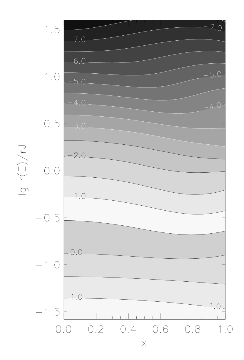
Figure 15: Distribution function in the energy–circularity plane derived for NGC 6703, in the luminous plus dark matter potential with $v_{c}(R_{m})=231{\rm\,km\,s^{-1}}$ shown as the middle solid line in the upper panel of Fig. 14. Energy is specified by the value of $r(E)$, where $E=\Phi(r)$, in units of the fitted Jaffe radius $r_{J}$, and the df is given in arbitrary logarithmic units. The last measured kinematic data point is located at $\lg r(E)/r_{J}=0.23$.

From Fig. 14 we conclude that the stellar distribution function in NGC 6703 is near-isotropic at the centre and then changes to slightly radially anisotropic at intermediate radii ($\mathchar 28940\relax\!=\!0.3-0.4$ at 30”, $\mathchar 28940\relax\!=\!0.2-0.4$ at 60”). It is not well-constrained near the outer edge of the data, where formally $\mathchar 28940\relax\!=\!-0.5-+0.4$, depending on the correct potential in the allowed range. However, the models with large asymptotic halo circular velocities shown in Fig. 14 appear less plausible, because they are the models with the most rapidly increasing velocity dispersions outside $R\simeq 60^{\prime\prime}$. The same models also show the most rapid increase in tangential anisotropy at and beyond $R_{m}=78^{\prime\prime}$, which again appears a priori implausible, because it implies rapid changes in the df just outside the observed range. The combined signature of both effects is strongly reminiscent of Fig. 9, where it was clearly an artifact of the limited radial range of the data. If this assumption is correct, one would again conclude that lower–$v_{c}(R_{m})$ models in the formal range are favoured. Fig. 15 shows the recovered df for the potential with $v_{c}(R_{m})=231{\rm\,km\,s^{-1}}$ in Fig. 14. Note, however, that all models shown in Fig. 14 except the self–consistent one are formally consistent with the presently available data.

Figure 16: Luminous, dark, and total mass as a function of radius for the range of acceptable models of NGC 6703, according to Fig. 12 (short dashed, dotted, and dash–dashed or full lines, respectively). Mass distributions in which a df with $\mathchar 28959\relax^{2}_{\mathchar 28955\relax+h4}\leq 1.12$ (including $87\%$ of the distribution in Fig. 7, $1.5\mathchar 28955\relax$) are coded by full lines, those with $\mathchar 28959\relax^{2}_{\mathchar 28955\relax+h4}\leq 1.28$ (including $95\%$, $2.0\mathchar 28955\relax$) by dash–dashed lines. The vertical line denotes the position of the last kinematic data point. At this radius, the luminous mass fails by at least a factor of $1.6$.

Figure 17: The B-band mass–to–light ratio of NGC 6703. The solid and dash–dashed lines (coding as in Fig. 16) are derived from the dynamical models that span the range of acceptable $v_{c}(R_{m})$ in Fig. 12. The central mass–to–light ratio is $\Upsilon=3.3$, that at the position of the last kinematic data point at 78” (vertical bar) is in the range of $\Upsilon=5.3-10$.

From the constraints on the circular velocity $v_{c}(R_{m})=210-290{\rm\,km\,s^{-1}}$ the range in mass inside $R_{m}=13.5\,h_{50}^{-1}{\rm\,kpc}$ is

$$M(<R_{m})=1.6-2.6\times 10^{11}h_{50}^{-1}{\rm\,M_{\odot}},$$ (17)

where $h_{50}\equiv H_{0}/50{\rm km/s/Mpc}$. The total mass in stars inside this radius is $8-9\times 10^{10}{\rm\,M_{\odot}}$, assuming constant mass-to-light ratio $\Upsilon$ and a maximum stellar mass model, and taking an average value from the models consistent with the kinematic data. The radial run of the luminous, dark, and total mass is shown in Fig. 16 for the models that span the allowed range according to Fig. 12. After dividing by the luminosity $L_{B}(r)$ for the stars, the mass-to-light ratios shown in Fig. 17 result. Between the centre and the last data point $r\!=\!78^{\prime\prime}\!\simeq\!2.6R_{e}$, the mass-to-light ratio of NGC 6703 rises by a factor of $1.6-3$.

5.3 Uncertainties

There are a number of possible sources of systematic error which would affect the mass–to–light ratio derived for NGC 6703. Most of the errors so introduced are probably small compared to the considerable uncertainty arising from the kinematic measurement errors and limited radial sampling, discussed above. One systematic error on the absolute mass-to-light ratios in NGC 6703 comes from the uncertainty in the distance, although this does not change the ratio of outer to central values. A further systematic effect on this ratio can be introduced by the sky brightness level: If this is increased by $2-3\%$, the fitted $r_{J}$ decreases to 35”. To the extent that the outermost kinematic data point at 78” (which then moves to larger $r/r_{J}$) is in the flat part of the circular rotation curve, the inferred M/L changes only to second order because the luminosity inside 78” remains essentially unchanged. The same is true if the sky value is decreased by $1\%$, in which case the fitted $r_{J}$ increases to $54^{\prime\prime}$.

In the previous analysis, we have ignored a possible small rotation in the outer parts of NGC 6703 (perhaps $\sim 20-30{\rm\,km\,s^{-1}}$ at $R\mathrel{\hbox to0.0pt{\lower 3.0pt\hbox{$\mathchar 536\relax$}\hss}\raise 2.0pt\hbox{$\mathchar 318\relax$}}50^{\prime\prime}$, but the errors are large; cf. Fig. 1). The simplest possible estimate of the effect of this rotation on the derived masses is to replace $\mathchar 28955\relax\simeq 105{\rm\,km\,s^{-1}}$ in this radial range by $(\mathchar 28955\relax^{2}+v^{2})^{1/2}\simeq 110{\rm\,km\,s^{-1}}$. This gives a factor of $1.1$, neglecting changes in the model structure that would result because the central kinematics remain unchanged.

Next we consider the possibility that NGC 6703 may contain a face-on extended disk (see de Vaucouleurs, de Vaucouleurs and Corwin 1976). From an $R^{1/4}$-law plus disk decomposition, we estimate that the contribution of such a disk in the region where we model the kinematics could be up to 10-20%. In this case we expect the velocity dispersion to be decreased and the $h_{4}$ coefficient to become more positive where the disk contributes significant light (Dehnen & Gerhard 1994; see NGC 4660 as an example in BSG), most likely in the outer parts.

Similarly, it is conceivable that NGC 6703 is in reality slightly triaxial and is seen from a special direction so as to appear E0. The likelihood of this is the smaller, the more triaxial the intrinsic axial ratios are; thus slightly triaxial shapes are the most plausible ones. Again this will imply some extra loop orbits seen nearly face-on, similarly increasing $h_{4}$ and decreasing $\mathchar 28955\relax$.

In both cases, we therefore expect the spherical component in NGC 6703 to have lower $h_{4}$ and larger $\mathchar 28955\relax$ than the measured values. A similar analysis of such kinematics would, according to the discussion in Section 3, lead to a model with greater tangential anisotropy at large radii, with the mass distribution less affected. Recall that decreasing the mass at large $r$ in a spherical model lowers both $\mathchar 28955\relax$ and $h_{4}$.

6 Discussion and Conclusions

This study is part of an observational and theoretical program aimed at understanding the mass distribution and orbital structure in elliptical galaxies. In the following we first discuss general results on potential and anisotropy determination, and then proceed to the specific case of NGC 6703.

6.1 Velocity profiles and anisotropy and mass

The analysis of the vps of simple dynamical models in Section 3 has broadly confirmed the conclusions of G93. At large radii, where the luminosity profile falls rapidly, the vps are dominated by the stars at tangent point. Then radially (tangentially) anisotropic dfs can be recognized by more peaked (more flat-topped) vps with more positive (negative) $h_{4}$ than for the isotropic case. Increasing $\mathchar 28940\relax$ at constant potential thus lowers $\mathchar 28955\relax$ and increases $h_{4}$. On the other hand, increasing the mass of the system at large $r$ at constant anisotropy, increases both the projected dispersion and $h_{4}$. This suggests that by modelling $\mathchar 28955\relax$ and $h_{4}$ both mass $M(r)$ and anisotropy $\mathchar 28940\relax(r)$ can be constrained.

In practical applications, such an analysis is complicated by a number of factors. Radial orbits at large radii may lead to increased central velocity dispersions and flat–topped central vps (already pointed out by Dejonghe 1987). The former effect can be compensated by a decrease in the stellar mass–to–light ratio. The latter is independent of this, but can be compensated by changes to the distribution function in the inner parts of the galaxy (as in a number of cases studied in Sections 4, 5). A more serious uncertainty is introduced by the possibility of significant gradients in the orbit population across the radii of interest. For example, a population of high energy radial orbits with pericentres in a limited radial range may mimic tangential anisotropy there. In many cases it will be possible to exclude such a population of orbits by its effects on the vps at exterior radii, i.e., by simultaneously analysing a number of observed vps. Yet this is least possible precisely at the largest observed radii, where mass determination is most interesting. Thus this chain of argument suggests (correctly, see below) that the largest uncertainty in determining masses and anisotropies in ellipticals from vp–data is the finite radial extent of these data.

To analyze realistic data we have constructed an algorithm by which the distribution function and potential of a spherical galaxy can be constrained directly from its observed $\mathchar 28955\relax$ and $h_{4}$–profiles. To assess the significance of the results obtained, we have tested the algorithm on Monte Carlo–generated data sets tuned to the spatial extent, sampling, and observational errors as measured for NGC 6703. From such data, the present version of the algorithm recovers a smooth spherical df, $\sim 70\%$ of the time, to an rms level of better than $\sim 12\%$ inside three times the radius of the outermost kinematic data point.

We have used this algorithm to study quantitatively the degree to which the gravitational potential can be determined from such data. Our main conclusion is that velocity profile data with presently achievable error bars already constrain the gravitational potentials of elliptical galaxies significantly. In particular, constant–M/L models are relatively easy to rule out once the data extend beyond $2R_{e}$. The examples that we have studied in detail, tuned to the NGC 6703 data, certainly belong to the less favourable cases, because in this galaxy the dispersion profile is falling.

A good way to parametrize the results is in terms of the true circular velocity $v_{c}(R_{m})$ at the radius of the outermost data point, $R_{m}$. With presently available data, $v_{c}(R_{m})$ can be determined to a precision of about $\pm\mathrel{\hbox to0.0pt{\lower 3.0pt\hbox{$\mathchar 536\relax$}\hss}\raise 2.0pt\hbox{$\mathchar 316\relax$}}50{\rm\,km\,s^{-1}}$. This will improve when high–quality data at several $R_{e}$ become available, of the kind expected from the new class of 10m telescopes. Apart from the fact that smaller error bars will decrease the formally allowed range in $v_{c}(R_{m})$, tests show that this range often includes high–$v_{c}(R_{m})$ models which become rapidly tangentially anisotropic just outside the data boundary. These (not very plausible) models can be eliminated with data extending to larger radii.

On the other hand, the detailed form of the true circular velocity curve is much harder to determine than $v_{c}(R_{m})$. Conspiracies in the df are possible that minimize the measurable changes in the line profile parameters. Our tests showed that two potentials differing by just the value of the halo core radius could not be distinguished even with very good data out to $6R_{e}$. Thus some uncertainty will remain in practise, regardless of whether or not in theory the potential is uniquely determined from the projected df $N(r,v_{\scriptscriptstyle\|})$.

A similar picture holds for the related determination of the anisotropy of the df. For the present error bars in the data, $\mathchar 28940\relax(r)$ is relatively well–determined out to about half the limiting radius of the observations. Near the edge of the data, uncertainties can be large depending on the gravitational potential (recall that in a fixed spherical potential, the df is uniquely determined by the complete projected df $N(r,v_{\scriptscriptstyle\|})$). Again the unknown nature of the orbits beyond the last data point has a large part in this uncertainty.

Because the largest uncertainties in determining masses and anisotropies from vps occur near the outer radial limit of these data, the combination of the type of analysis presented here with other information (e.g., from X-ray data) will be particularly powerful.

6.2 The dark halo of NGC 6703

Fig. 10 shows that no self-consistent model will fit the kinematic data for NGC 6703. Our non–parametric best–estimate self–consistent model is inconsistent with the data at the $>99\%$–level (Figs. 12, 7). With self-consistent models, either the velocity dispersion profile is matched reasonably well, but then the line profiles cannot be reproduced, or, when the $h_{4}$-profile is fitted accurately, the dispersion profile is poorly matched. The cure for the discrepancy is to raise both $\mathchar 28955\relax$ and $h_{4}$ at large radii. Thus, as discussed above, we require extra mass at large $r$. NGC 6703 must have a dark halo.

We have next derived constraints on the parameters of this halo as follows. The luminous component is assigned a constant mass-to-light ratio $\Upsilon$, chosen maximally such that the stars contribute as much mass in the center as is consistent with the kinematic data. Our parametric model for the halo incorporates a constant density core, and its parameters (core radius $r_{c}$ and asymptotically constant circular velocity $v_{0}$) are chosen such the halo adds mass mainly in the outer parts of the galaxy if that is necessary. We call these models maximum stellar mass models (analogous to the maximum disk hypothesis in the analysis of disk galaxy rotation curves).

We find that maximum stellar mass models in which the luminous component provides nearly all the mass in the centre fit the data well. In these models, the total luminous mass inside the limiting observational radius $R_{m}\!=\!78^{\prime\prime}\!=\!13.5\,h_{50}^{-1}{\rm\,kpc}$ is $9\times 10^{10}h_{50}^{-1}{\rm\,M_{\odot}}$, corresponding to a central B–band mass–to–light ratio $\Upsilon=3.3h_{50}{\rm\,M_{\odot}}/{\rm\,L_{\odot}}$. According to Worthey’s (1994) models, this is a rather low value for the stellar population of an elliptical galaxy and would point to a relatively low age (5 Gyrs) and/or low metallicity (less than solar). However, the galaxy has a color $(B-V)_{0}=0.93$ and a central line index $Mg_{2}=0.280$ (Faber et al. 1989) which are typical for ellipticals of similar velocity dispersion.

A larger value of $H_{0}$ could increase the M/L value and alleviate the demands on the stellar populations. However, the distance used here (36 Mpc) includes a correction for the large inferred peculiar velocity of the galaxy. If we had used a distance based on the larger radial velocity in the CMB frame, our derived M/L would be even lower. It is also implausible that the low central value of M/L stems from the contribution of a young stellar population in a disk component, which we estimate cannot be larger than $20\%$ of the total light (see above). Thus we conclude that the dark halo in NGC 6703 is unlikely to have higher central densities than inferred from our maximum stellar mass models, because otherwise the M/L of the stellar component would be reduced to implausibly small values.

In a recent preprint, Rix et al. (1997) have analyzed the velocity profiles of the E0 galaxy NGC 2434 with a linear orbit superposition method. This galaxy provides an interesting contrast to NGC 6703 because it has an essentially flat dispersion profile. Its kinematics are likewise inconsistent with a constant–M/L potential, but are well–fit by a model with $v_{c}\!=\!{\rm const}$. This can be interpreted as a maximum stellar mass model in the sense defined above, in which the luminous component with maximal $\Upsilon$ contributes most of the mass inside $R_{e}$. The kinematics of NGC 2434 are also well–fit by a range of specific, cosmologically motivated mass models which, if applicable, would imply lower $\Upsilon$ and significant dark mass inside $R_{e}$. In NGC 6703, a model with $v_{c}\!=\!{\rm const}$ is formally consistent with the present data (within $2\mathchar 28955\relax$), but it is not a very plausible fit at large $R$ and requires large anisotropy gradients between 40” and 70”. It will be interesting to see whether future studies confirm differences between the shapes of the true circular velocity curves of elliptical galaxies.

Because of the falling dispersion curve in NGC 6703, we can determine only one of the halo parameters (The halo parameters of the most probable potentials lie in a band extending from low $v_{0}$ and low $r_{c}$ to high $v_{0}$ and high $r_{c}$.) However, the circular velocity $v_{c}(R_{m})$ at the data boundary is relatively well–determined for all these models. Thus we find (Fig. 12) that the true circular velocity of NGC 6703 at 78” is $v_{c}(R_{m})=250\pm 40{\rm\,km\,s^{-1}}$ (formal $95\%$ confidence interval). Tests on pseudo data have shown that this range often includes high–$v_{c}(R_{m})$ models which become rapidly tangentially anisotropic just outside the data boundary. Such models may not be very plausible, so the lower values in the quoted range of $v_{c}(R_{m})=250\pm 40{\rm\,km\,s^{-1}}$ may be the more probable ones.

Thus, at $R_{m}\!=\!78^{\prime\prime}\!=\!13.5\,h_{50}^{-1}{\rm\,kpc}$ the total mass enclosed is $M(<R_{m})=1.6-2.6\times 10^{11}h_{50}^{-1}{\rm\,M_{\odot}}$, and the integrated mass–to–light ratio out to this radius is $\Upsilon=5.3-10$, corresponding to a rise from the center by at least a factor of $1.6$. We have already noted that NGC 6703 is an unfavourable case because of its falling dispersion curve. The fact that relatively small variations in $\Upsilon$ can nonetheless be detected shows the power of the method. Note that a scheme based on the analysis of the line of sight velocity dispersions alone (Binney, Davies, Illingworth 1990, van der Marel 1991) would conclude that constant mass–to–light ratio models can provide good fits.

The stellar distribution function in NGC 6703 is near-isotropic at the centre and then changes to slightly radially anisotropic at intermediate radii ($\mathchar 28940\relax\!=\!0.3-0.4$ at 30”, $\mathchar 28940\relax\!=\!0.2-0.4$ at 60”). It is not well-constrained near the outer edge of the data, where formally $\mathchar 28940\relax\!=\!-0.5-+0.4$, depending on the correct potential in the allowed range. Models near the lower end of this range may be consistent with the data only because of the limited radial extent of the measurements.

6.3 Conclusions

In summary, we have shown that the mass distribution $M(r)$ and anisotropy structure $\mathchar 28940\relax(r)$ for spherical galaxies can both be constrained from vp and velocity dispersion measurements. NGC 6703 must have a dark halo, contributing about equal mass at $2.6R_{e}$ as do the stars. The circular velocity at the last kinematic data point (78”) is constrained to lie in the range $250\pm 40{\rm\,km\,s^{-1}}$ at $95\%$ confidence. The anisotropy of the stellar orbits changes from near-isotropic at the center to slightly radially anisotropic at intermediate radii, and may be either radially or tangentially anisotropic at 78”. With more extended and more accurate data it will be possible to considerably narrow down these uncertainties.

If the results for this galaxy are typical, they suggest that also in elliptical galaxies the stellar mass dominates at small radii, and the dark matter begins to dominate at radii around $10{\rm\,kpc}$. It is important to obtain extended kinematic data and do a similar analysis for a number of elliptical galaxies. When we know the systematics and the spread in the circular velocity curves and anisotropy profiles for a sample of ellipticals, we will have an important new means for testing the currently popular formation theories.

Appendix A: Library of anisotropic spherical distribution functions

To understand the connection between anisotropy structure and observable line profile shapes we have constructed a number of spherical distribution functions of the quasi–separable form (Gerhard 1991, G91)

$$f(E,L)=g(E)\;h(x),$$ (18)

where the variable $x$ depends on both energy and angular momentum:

$$x={L\over L_{0}+L_{c}(E)}.$$ (19)

$L_{0}$ is an angular momentum constant, or equivalently, an anisotropy radius times a characteristic velocity; $L_{c}(E)$ is the angular momentum of the circular orbit at energy $E$. dfs of the form (18) have the following properties: (i) the circularity function $h(x)$ has the effect of shifting stars between orbits of different angular momenta on surfaces of constant energy, while $g(E)$ controls the distribution of stars between energy surfaces. (ii) For the most bound stars $L<L_{c}(E)\ll L_{0}$; thus the model becomes isotropic in the centre unless $L_{0}\!=\!0$. (iii) For loosely bound stars $L\sim L_{c}(E)\gg L_{0}$, i.e., the angular momentum distribution becomes a function of circularity $L/L_{c}(E)$ which is one-to-one related to orbital eccentricity. Outside the anisotropy radius, the df (18) therefore corresponds to an energy-independent orbit distribution with constant anisotropy, radial or tangential.

In these models $h(x)$ is an assigned function built into the model to achieve the desired anisotropy (orbit distribution). Radially biased distribution functions correspond to circularity functions $h(x)$ decreasing with $x$; for example

$$h(x)=h_{\mathchar 28939\relax}(x)\equiv\left(1-x^{2}\right)^{\mathchar 28939\relax}.$$ (20)

The family can also be used to construct tangentially anisotropic models, such as

$$h_{c,\mathchar 28939\relax}(x)=c+(1-c)\left[1-(1-x^{2})^{\mathchar 28939\relax}\right].$$ (21)

In these tangentially anisotropic models one cannot choose $h(0)=0$ unless $L_{0}=0$, otherwise the density at $r\!=\!0$ would be zero. Of course, other forms for $h(x)$ are possible, such as Gaussians.

Figure 18: Anisotropy parameter $\mathchar 28940\relax(r)$, projected velocity dispersion $\mathchar 28955\relax_{p}$, and line profile shape parameter $h_{4}$ for several families of anisotropic dfs. Left: scale–free radially anisotropic (dotted) and tangentially anisotropic (dashed lines) in the potential of a self–consistent Jaffe sphere. For these models, circularity functions of the type (20) and (21) were used with different $\mathchar 28939\relax$ and $c$, respectively. The isotropic model is shown for reference (solid line). Right: Families of models with anisotropy changing from radial to tangential (dotted) or from tangential to radial (dashed lines). These were constructed from the same circularity functions and a weight factor as in eq. (23).

Given the assigned function $h(x)$, the integral equation for $\mathchar 28954\relax(r)$ in terms of $f(E,L^{2})$ is solved for the derived function $g(E)$; see G91 and Jeske (1995). Fig. 3 shows line profile shape parameters for representative dfs constructed in this way. Fig. 3 shows the anisotropy profiles of two sets of tangentially anisotropic models. Here the density of stars has been taken to be that of a Jaffe sphere, and the potential in which the stars orbit is either the self–consistent potential or one of the mixed stars plus halo potentials used in Sections 4, 5. Sequences like that in Fig. 3 are used as basis functions in the non–parametric analysis in Section 5.

Models whose anisotropy changes from radial to tangential or vice versa were constructed by linearly combining the above circularity functions with energy–dependent coefficients. In this way one obtains dfs of the more general form

$$f(E,L)=g(E)\;h(E,x).$$ (22)

For self–consistent Jaffe models we used energy–dependent coefficients $\mathchar 28950\relax(E)$ of the following form:

$$\mathchar 28950\relax(E)={1\over 2}+{1\over\mathchar 28953\relax}\arctan{\left[{k\over 2}{E^{2}-\overline{E}^{2}\over E^{2}}\right]}.$$ (23)

The parameters $\overline{E}$ and $k$ determine the orbital energy near which the anisotropy transition occurs, and the width of the transition. A similar function $\mathchar 28950\relax(E)$ was used for models in halo potentials. Figure 18 shows the intrinsic and projected properties of a number of dfs of this kind, constructed in the self–consistent potential of a Jaffe sphere. Notice the wide variety of kinematical profiles that can be constructed in this way.

Appendix B: Transforming to linear kinematic data

In velocity line profile measurements, the depth of an absorption line in a spectral resolution element is assumed to be proportional to the number of stars with line-of-sight velocities corresponding to this wavelength interval. The line-of-sight velocity distribution measured from the line profiles is a discretized function linearly related to the underlying df [cf. eq. (1)]. This linearity is lost when line profile measurements are represented by the quantities $v$, $\mathchar 28955\relax$, $h_{3}$, $h_{4}$ — these quantities are obtained by a least-square fit of a Gauss-Hermite series to the observed line profile.

To re-express the observed kinematics in terms of quantities that depend linearly on $f$ we proceed as follows. Consistent with the assumption of spherical symmetry, we set the mean streaming velocity $\overline{v}$ and all odd velocity profile moments to zero. Next, we obtain an estimate for the velocity dispersion (second moment) $\overline{\mathchar 28955\relax}^{2}$, by integrating over the line profile specified by $(\mathchar 28955\relax,h_{4})$; for negative $h_{4}$, until it first becomes zero. For small $h_{4}$, the linear correction formula $\overline{\mathchar 28955\relax}\!=\!\mathchar 28955\relax(1+\sqrt{6}h_{4})$ holds (van der Marel & Franx 1993), this correction results in $\overline{\mathchar 28955\relax}\!>\!\mathchar 28955\relax$ for peaked profiles with $h_{4}\!>\!0$. The numerical correction from integrating over the velocity profile also has this property (BSG).

From the measured $h_{4}(R_{i})$, we compute new even Gauss-Hermite moments $s_{n}(R_{i};\widetilde{\mathchar 28955\relax})$ by expanding the series

$${\cal L}(R_{i},v_{\scriptscriptstyle\|})={\cal L}_{0}\sum_{j=0,4}h_{j}(R_{i})\,H_{j}(x)\,\exp(-x^{2}/2)$$ (24)

($h_{0}\!=\!1$, $h_{1}\!=\!h_{2}\!=\!h_{3}\!=\!0$) with $x\equiv v_{\scriptscriptstyle\|}/\mathchar 28955\relax(R_{i})$ as

$${\cal L}(R_{i},v_{\scriptscriptstyle\|})=\!\sum_{n=0,2,4,...}\!\!\!N_{n}\,s_{n}\,H_{n}(\widetilde{x})\,\exp(-\widetilde{x}^{2}/2),$$ (25)

where $\widetilde{x}\equiv v_{\scriptscriptstyle\|}/\widetilde{\mathchar 28955\relax}(R_{i})$. Here $H_{n}$ are Hermite polynomials, the $N_{n}$ are normalization constants (G93), and $\widetilde{\mathchar 28955\relax}(R_{i})$ are fiducial scaling velocities generally different from $\overline{\mathchar 28955\relax}(R_{i})$. In practice, we have found it convenient to take for $\widetilde{\mathchar 28955\relax}(R_{i})$ the velocity dispersions $\mathchar 28955\relax_{\rm iso}(R_{i})$ of the isotropic model in the given potential $\Phi(r)$ with the same stellar density as the galaxy being analyzed. The $s_{n}(R_{i};\widetilde{\mathchar 28955\relax})$ are estimates for the Gauss-Hermite moments related to the true velocity profile by

$$s_{n}(R_{i};\widetilde{\mathchar 28955\relax}) = \left(2^{n-1}n!\right)^{-1/2}$$

$$\times\int_{-\infty}^{\infty}\!dv_{\scriptscriptstyle\|}\,H_{n}(v_{\scriptscriptstyle\|}/\widetilde{\mathchar 28955\relax})\,\exp(-v_{\scriptscriptstyle\|}^{2}/2\widetilde{\mathchar 28955\relax}^{2})\,{\cal L}(R_{i},v_{\scriptscriptstyle\|}).$$

For a theoretical model, we obtain corresponding moments by inserting the projected df $N(R_{i},v_{\scriptscriptstyle\|})$ from (1) into eq. (26) instead of ${\cal L}(R_{i},v_{\scriptscriptstyle\|})$, using the same $\widetilde{\mathchar 28955\relax}(R_{i})$. Clearly, the new $s_{n}$-moments of the composite model are linear in the $a_{k}$, i.e.,

$$s_{n}(R_{i};\widetilde{\mathchar 28955\relax})=\sum_{k=1,K}a_{k}s_{n}^{(k)}(R_{i};\widetilde{\mathchar 28955\relax})$$ (27)

with the $s_{n}^{(k)}$ corresponding to the respective $f_{k}$.

References

- [Awaki et al. , 1994] Awaki H., et al. , 1994, PASJ 46, L65
- [Arnaboldi et al. , 1994] Arnaboldi M., Freeman K.C., Hui X., Capaccioli M., Ford H., 1994, Messenger 76, 40
- [Bender, 1990] Bender R., 1990, A&A 229, 441
- [Bender, Saglia & Gerhard, 1994] Bender R., Saglia, R., Gerhard, O.E., 1994, MNRAS 269, 785 (BSG)
- [Binney, 1978] Binney J.J., 1978, MNRAS 183, 501
- [Binney, Davies & Illingworth 1990] Binney, J.J., Davies, R.L., Illingworth, G.D., 1990, ApJ 361, 78
- [Binney & Mamon, 1982] Binney J.J., Mamon G.A., 1982, MNRAS 200, 361
- [Carollo et al. , 1995] Carollo C.M., de Zeeuw P.T., van der Marel R.P., Danziger I.J., Qian E.E., 1995, ApJL 441, L25
- [Dehnen & Gerhard 1994] Dehnen W., Gerhard O.E., 1994, MNRAS 268, 1019
- [Dejonghe, 1987] Dejonghe H., 1987, MNRAS 224, 13
- [Dejonghe et al. , 1996] Dejonghe H., de Bruyne V., Vauterin P., Zeilinger W.W., 1996, A&A 306, 363
- [Dejonghe & Merritt, 1992] Dejonghe H., Merritt D., 1992, ApJ 391, 531
- [de Vaucouleurs et al. , 1976] de Vaucouleurs G., de Vaucouleurs A., Corwin H.G., 1976, Second Reference Catalogue of Bright Galaxies, Univ. Texas Press, Austin
- [Faber et al. , 1989] Faber S.M., Wegner G., Burstein D., Davies R.L., Dressler A., Lynden-Bell D., Terlevich R.J., 1989, ApJS 69, 763
- [Franx, van Gorkom & de Zeeuw, 1994] Franx M., van Gorkom J.H., de Zeeuw T., 1994, ApJ 436, 642
- [Fricke, 1952] Fricke W., 1952, Astr. Nachr. 280, 193
- [Gerhard, 1991] Gerhard O.E., 1991, MNRAS 250, 812 (G91)
- [Gerhard, 1993] Gerhard O.E., 1993, MNRAS 265, 213 (G93)
- [Grillmair et al. , 1994] Grillmair C.J., Freeman K.C., Bicknell G.V., Carter D., Couch W.J., Sommer-Larsen J., Taylor K., 1994, ApJ 422, L9
- [Hanson & Haskell 1981] Hanson R.J., Haskell K.H., 1981, Math. Programm. 21, 98.
- [Jaffe, 1983] Jaffe W., 1983, MNRAS 202, 995
- [Jeske, 1995] Jeske, G., 1995, PhD Thesis, University of Heidelberg
- [Jeske et al. , 1996] Jeske, G., Gerhard, O.E., Bender, R., Saglia, R.P., 1996, Proc. IAU 171, eds. Bender, R., Davies, R.L., p. 397
- [Kim & Fabbiano, 1995] Kim D.-W., Fabbiano G., 1995, ApJ 441, 182
- [Kochanek & Keeton, 1997] Kochanek C.S., Keeton C.R., 1997, in The Nature of Elliptical Galaxies, Stromlo Symposium, eds. Arnaboldi M., Da Costa G.S., Saha P., 1997, ASP 116, 21.
- [Maoz & Rix, 1993] Maoz D., Rix H.-W., 1993, ApJ 416, 435
- [Merritt, 1985] Merritt D., 1985, AJ 90, 1027
- [Merritt, 1993] Merritt D., 1993, ApJ 413, 79
- [Osipkov, 1979] Osipkov L.P., 1979, Pis’ma Astr. Zh. 5, 77
- [Press et al. , 1986] Press, W.H., Flannery, B.P., Teukolsky, S.A., Vetterling, W.T., Numerical Recipes (Cambridge: Cambridge University Press)
- [Rix et al. 1997] Rix H.-W., de Zeeuw P.T., Carollo C.M., Cretton N., van der Marel R.P., 1997, preprint
- [Saglia et al. , 1993] Saglia R.P. et al. , 1993, ApJ 403, 567
- [Saglia et al. , 1997b] Saglia, R.P., Bender, R., Gerhard, O.E., Jeske, G., 1997a, in Dark and Visible Matter in Galaxies and Cosmological Implications, eds. Persic M., Salucci P., ASP 117, 113.
- [Saglia et al. , 1997b] Saglia R.P. et al. , 1997b, ApJS 109, 79
- [van der Marel, 1991] van der Marel, R., 1991, MNRAS 253, 710
- [van der Marel & Franx, 1993] van der Marel R.P., Franx M., 1993, ApJ 407, 525
- [Worthey 1994] Worthey, G. 1994, ApJS, 95, 107