New aspects of absorption line formation in intervening turbulent clouds – III. The inverse problem in the study of H+D profiles

Abstract

A new method, based on a Reverse Monte Carlo technique and aimed at the inverse problem in the analysis of interstellar (intergalactic) absorption lines is presented. We consider the process of line formation in media with a stochastic velocity field accounting for the effects of a finite correlation length (mesoturbulence). This approach generalizes the standard microturbulent approximation, which is commonly used to model the formation of absorption spectra in turbulent media.

The method allows to estimate from an observed spectrum both, the physical parameters of the absorbing gas, and an appropriate structure of the velocity distribution parallel to the line of sight. The procedure is applied to a template H+D Ly$\alpha$ profile which reproduces the Burles & Tytler [B&T] spectrum of the quasar Q 1009+2956 with the DI Ly$\alpha$ line seen at the redshift $z_{a}=2.504$.

The results obtained favor a low D/H ratio in this particular absorption system, although the inferred upper limit for the hydrogen isotopic ratio of about $4.6\times 10^{-5}$ is slightly higher than that of B&T [log (D/H) = $-4.60\pm 0.08\pm 0.06$, i.e. D/H$\la 3.47\times 10^{-5}$]. This revision of the B&T data in the framework of the mesoturbulent model leads to limits on D/H consistent with standard big bang nucleosynthesis [SBBN] predictions and observational constraints on both extra-galactic ⁴He mass fraction Y_p (Izotov et al. 1997) and ⁷Li abundance in the atmospheres of population II (halo) stars (Bonifacio & Molaro 1997). SBBN restricts the common interval of the baryon to photon ratio $\eta$ for which there is concordance between the various abundances to $3.9\times 10^{-10}\la\eta\la 5.3\times 10^{-10}$. It implies that $0.014\la\Omega_{b}h^{2}\la 0.020$, where $h$ is the Hubble constant in units 100 km s^-1 Mpc^-1.

1 Introduction

In two previous papers (Levshakov & Kegel 1997, and Levshakov, Kegel & Mazets 1997, Paper I and II hereinafter, respectively), we investigated the formation of absorption lines in chaotic media with finite correlation length of the velocity field (mesoturbulence), when the observed absorption spectra correspond to only one line of sight. We have shown that accounting for a finite correlation length in the large scale stochastic velocity field changes the interpretation of absorption spectra considerably. The line profiles, as well as the equivalent widths, may be strongly affected by the correlations. Therefore the standard analysis of absorption spectra based on the microturbulent approximation and the Voigt profile fitting procedure may yield misleading results concerning the physical parameters of the absorbing gas (for numerous examples, see Levshakov & Kegel 1994, 1996; Levshakov & Takahara 1996a,b; Paper I and Paper II). At least one can say that the results obtained by the standard analysis are model dependent and, thus, are not unique.

In our cloud model we account for a stochastic velocity field with finite correlation length $l$ but assume the absorbing material to be homogeneous in density and temperature. The model is fully defined by specifying the column density $N$, the kinetic temperature $T_{kin}$, the ratio of the r.m.s. turbulent velocity to the thermal velocity $\sigma_{t}/v_{th}$, the ratio of the cloud thickness to the correlation length $L/l$, as well as one realization of the velocity field distribution along the line of sight. Because of the very large time scale for changes in the hydrodynamic flows the random structure of the velocity field along a given line of sight has to be considered as ‘frozen’ over the exposure time. It follows that the observed absorption spectrum in the light of a point-like source (star, QSO) corresponds to only one realization of the velocity field. Therefore, the intervening absorption spectrum cannot be considered as a time or space average in the statistical sense. This means that the actual distribution of the hydrodynamic velocities at a given instant of time corresponds to an incomplete sample and, thus, may deviate from the average distribution function assumed to be Gaussian. Accordingly, significant deviations from the expected average intensity $\langle I_{\lambda}\rangle$ can occur. – For this reason we used in Paper II a Monte Carlo technique to calculate spectra corresponding to the absorption along individual lines of sight.

In Paper II we considered the direct problem, i.e. we specified the physical parameters and generated individual random realizations of the velocity distribution [more exactly – the distribution of the velocity component parallel to the line of sight $v(s)$] with which we then calculated individual spectra. The aim of the present paper is the inverse problem, i.e. the problem to deduce physical parameters from an observed spectrum. To reproduce a given (observed) spectrum within the framework of our model, one has to find the proper physical parameters and an appropriate realization of the velocity field. In general, $v(s)$ is a continuous random function of the coordinate $s$, but in the numerical procedure it is sampled at evenly spaced intervals $\Delta s$. The necessary number of intervals depends on the values of $\sigma_{t}/v_{th}$ and $L/l$, being typically $\sim 100$ for hydrogen absorption lines. Thus, to estimate model parameters from the observed spectrum one has to solve an optimization problem in a parameter space of very large and variable (depending on $\sigma_{t}/v_{th}$, $L/l$) dimension. It is known that such kind of problems may be solved using stochastic optimization methods. The Reverse Monte Carlo [RMC] technique based on the computational scheme invented by Metropolis et al. (1953) proved to be adequate in our case. The method is successfully used in many applications where the state space of a physical system is huge (see e.g. Press et al. 1992, or Hoffmann 1995).

We apply the RMC method to the problem of determining the primordial deuterium abundance at high redshift. In particular, the H+D Ly$\alpha$ profile observed by Burles & Tytler (1996, B&T hereinafter) in the spectrum of the quasar Q 1009+2956 is considered. This spectrum was selected since ($a$) it shows a pronounced DI absorptions at the redshift $z_{a}=2.504$, ($b$) it was obtained with high signal-to-noise ratio and spectral resolution, and ($c$) the total hydrogen column density estimated by B&T from the intensity level beyond the Lyman limit in this system is consistent with the normalized intensities in the HI Ly$\alpha$ wings.

In the present paper we extend our study of the accuracy of the D/H ratio determinations from our Galaxy (Paper II) to the very distant Ly$\alpha$-systems (putative intervening galaxies). The background source is supposed to be point-like and even in the case of distant QSOs we consider absorption along one line of sight only. This means that any gravitational focusing which may, in principle, lead to an additional spatial averaging over different lines of sight (an example may be found in Frye et al. 1997) is not taken into account. (The average mesoturbulent H+D Ly$\alpha$ spectra have been considered by Levshakov & Takahara 1996a.)

In Section 2 a description of the RMC method and the procedure to test its validity are given, while in Section 3 the method is applied to analyze an observed H+D Ly$\alpha$ spectrum. The results obtained are summarized in Section 4.

2 The Reverse Monte-Carlo method

The RMC method belongs to the class of stochastic optimization algorithms developed to solve optimization problems with a very large number of free parameters. Contrary to the standard Monte-Carlo procedure in which random configurations of a given physical system are generated to estimate its average characteristics, the RMC takes an experimentally determined set of data and searches for a parameter configuration which reproduces the observational data.

The inverse problem is always an optimization problem in which an objective function is minimized. The objective function defined over a space of very large dimension is known to have many local minima. Therefore optimization methods based on the choice of ‘minimization direction’ (so-called gradient methods) may fail because of the possibility of being trapped in one of such minima. The RMC approach allows to overcome this problem. It can get over the local minima because it does not use any concept of ‘direction’. Applied to the analysis of absorption spectra, the RMC method may be formulated as follows.

Figure 1: (a) – A Monte-Carlo simulation of the H+D Ly$\alpha$ profile. The thicker curve marks the blue wing of the HI line and the complex structure of the D absorption. (b) – The portion of the H+D profile marked in panel a is shown by open circles having error bars corresponding to S/N = 30 at the continuum level, while the solid curve is the result of the RMC minimization. (c) – The adopted one-dimensional velocity distribution (dotted curve) and the one determined by the RMC procedure (solid curve). (d) – Histograms $p(u)$ for the adopted (dotted lines) and estimated (solid lines) projected velocity distributions ($u\equiv v/\sigma_{t}$).

2.1 Computational procedure

The total parameter space consisting of the physical parameters (like $N,T_{kin},$ etc.) and the velocity components $v_{j}$ parallel to the line of sight at the individual positions $s_{j}$, is divided into two subspaces.

Let $\Theta=\{\hat{\theta}\}$ represent the subspace of physical parameters {$N,T_{kin},\sigma_{t}/v_{th},L/l$}. For the special case of H+D Ly$\alpha$  that we want to investigate, ${\hat{\theta}}$ has to have one additional component D/H – the ratio of the DI to HI column densities.

Let further $\{{\hat{v}}\}=\{v_{1},v_{2},\ldots,v_{k}\}$ be the vector of the velocity components parallel to the line of sight at the spatial points $s_{j}$, determined by the recurrent sequence (see Paper II)

$$v_{j}\equiv v(s_{j-1}+\Delta s)=\xi\sigma_{t}\sqrt{1-f^{2}}+fv_{j-1}\,,\,j=2,3,\ldots,k\,.$$ (1)

Here

$$f\equiv f(\Delta s)=\exp(-|\Delta s|/l)$$ (2)

is the correlation function and $\xi$ is a random number picked from a normal distribution with $\langle\xi\rangle=0$ and Var($\xi$) = 1.

For a chosen ${\hat{\theta}}$  and velocity field distribution the objective function ${\cal L}$ is calculated according to

$${\cal L}\equiv\chi^{2}=\frac{1}{\nu}\sum^{m}_{i=1}\left[\frac{I(\lambda_{i})-r(\lambda_{i})}{\sigma_{i}}\right]^{2}\,,$$ (3)

where $r(\lambda_{i})$ is the simulated random intensity [eq.(19) in Paper II],  $I(\lambda_{i})$ the observed normalized intensity within the $i$th pixel of the line profile, $\sigma_{i}$ an estimate of the experimental error, and $\nu=m-n$   the degree of freedom ($m$ is the number of data points and $n$ is the number of fitted physical parameters, $n=5$ in our case).

The minimization of $\chi^{2}$ is the main goal of the procedure. Any parameter configuration with $\chi^{2}\sim 1$ has to be considered as a physically reasonable model for the interpretation of the observational data.

The computational RMC procedure is split into two steps. At first, random values for the physical parameters are chosen, i.e. the vector ${\hat{\theta}}$. Secondly, an optimal velocity field configuration is estimated for these parameters. The current $\chi^{2}$ value is computed and if it is larger than $\chi^{2}_{\nu,\alpha}$ (which is the value of $\chi^{2}_{\nu}$ for a given credible probability $P_{\alpha}=1-\alpha$) the whole procedure is repeated. In principle, to choose the vector ${\hat{\theta}}$ in the physical parameter subspace we could use any of the common optimization methods (like e.g. nonlinear simplex) but we apply the same stochastic RMC procedure for both stages of the computational scheme. In detail it is described as follows.

1) A simulation box in the parameter subspace is specified by fixing the parameter boundaries.

2) ${\hat{\theta}}$ is chosen arbitrarily in the simulation box.

Next, the points 3–5 describe the evaluation of optimal velocity field configurations for a given set of physical parameters.

3) A random realization of the velocity field is generated, and the corresponding value of $\chi^{2}$ is calculated.

4) Subsequently an element $v_{j}$ is chosen at random, and a random change is given to this element in accord with (1). If $j$ happens to be equal to 1, we put $v_{1}=\xi\sigma_{t}$.

5) The new value of ${\cal L}$ is calculated. If $\Delta{\cal L}<0$, i.e. if $\chi^{2}_{new}<\chi^{2}_{old}$, the new ‘trial’ configuration of the velocity field is accepted. If $\Delta{\cal L}>0$, the trial configuration is accepted with a probability $P_{\Delta{\cal L}}=\exp(-\frac{1}{2}\Delta{\cal L})$, i.e. we take a random number $\zeta$ uniformly distributed in (0,1), and if $\zeta<P_{\Delta{\cal L}}$, the new configuration is accepted. If $\zeta>P_{\Delta{\cal L}}$, the change is rejected and the configuration of the velocity field is returned back to its previous state. Then we repeat the procedure from step (4) up to $\beta_{1}$ times to find the best solution (i.e. the smallest $\chi^{2}$ value) for the ${\hat{\theta}}$ under consideration. $\beta_{1}$ is chosen such that each $v_{j}$ has been changed on average so often that Var($v_{j})\sim\sigma^{2}_{t}$. – The procedure is stopped when $\chi^{2}\la\chi^{2}_{\nu,\alpha}$.

6) An element $\theta_{i}$ of ${\hat{\theta}}$ is chosen at random, a random change $\Delta\theta_{i}$ is given to it, and the procedure starting from step (3) is repeated (up to $\beta_{2}$ times) until $\chi^{2}_{min}$ will be less than an expected value $\chi^{2}_{\nu,\alpha}$. If after $\beta_{2}$ repetitions the condition $\chi^{2}_{min}<\chi^{2}_{\nu,\alpha}$ is not satisfied the procedure stops. $\beta_{2}$ is chosen such that each $\theta_{i}$ has been changed on average no less than 30 times to get a representative statistics.

Note that the convergence of the scheme depends on the size of the simulation box. The necessary size is unknown a priori. If it is too large, the computing time increases considerably, and if it is too small, the required $\chi^{2}$ value may not be reached at all. Therefore the box size must be chosen with some care and should be adjusted to the experimental data.

2.2 Validity of the RMC simulations

In order to test the validity of our RMC-computer code, we performed several tests in which the ‘observational’ H+D Ly$\alpha$ profile was generated for a given set of the parameters ${\hat{\theta}}\equiv$ { $N_{\rm HI}=2.5\times 10^{17}\ {\rm cm}^{-2}$, D/H = $1.5\times 10^{-4}$, $T_{kin}=1250$ K, $\sigma_{t}/v^{\rm H}_{th}=2.0$, $L/l=5.0$ }, and for one random realization of the one-dimensional velocity distribution. The chosen parameters are typical for the warm diffuse interstellar gas (cf. Linsky et al. 1995) except for the D/H ratio which was taken approximately 10 times larger than the mean ISM value in order to make the deuterium absorption being more pronounced in the simulated spectrum.

The test was conducted with the aim of evaluating whether the code is capable of finding the correct ${\hat{\theta}}$ and the correct structure of the stochastic velocity field. At first we considered a very soft constraint on the possible shape of the $v(s)$ distribution. Namely, only the blue wing of the H+D Ly$\alpha$ blend was used in the minimization procedure (this may correspond to the case when the red wing of the hydrogen profile is distorted by the Ly$\alpha$ forest lines). We will see later (Section 3) that the uncertainty range of the D/H ratio determination found under this soft constraint may be considerably reduced by accounting for the shape of the whole H+D Ly$\alpha$ absorption.

Figure 2: The contribution from different volume elements to the HI and DI local absorption coefficients for three fixed wavelengths $\lambda=1215.279$ Å (a1,a2), 1215.316 Å (b1,b2), and 1215.363 Å (c1,c2), which correspond to the two minima and the maximum inbetween in the DI profile shown in Fig. 1a.

Fig. 1a shows our simulated spectrum of H+D Ly$\alpha$. The example exhibits a complex intensity structure in DI. This complexity is caused by the finite correlation length effect only and, hence, it should not be interpreted as being caused by several (at least three) independent cloudlets with different radial velocities and different physical parameters. The velocity field distribution yielding this spectrum is shown in Fig. 1c by the dotted curve.

In order to illustrate the effects the correlated structure of the velocity field has on the line forming process, Fig. 2 shows the local absorption coefficient $k_{\lambda}(s)$ for HI and DI Ly$\alpha$ for three fixed wavelength $\lambda\simeq 1215.28,1215.32$ and 1215.36 Å  which correspond to the two minima and the maximum between them in the DI profile shown in Fig. 1a.

The correlations have the effect that for a given value of $\lambda$ the absorption coefficient may vary strongly along the line of sight. At the wavelengths chosen this effect is most pronounced for DI. This is in strong contrast to the microturbulent model (having the same $\sigma_{t}$ and $T_{kin}$) in which the whole region along the line of sight would evenly contribute to the absorption at a given $\lambda$. This is clearly seen from the hydrogen absorption coefficients which at the chosen wavelengths, lie in the range of the damping wing where both micro- and mesoturbulent models have the same solutions (see Paper II).

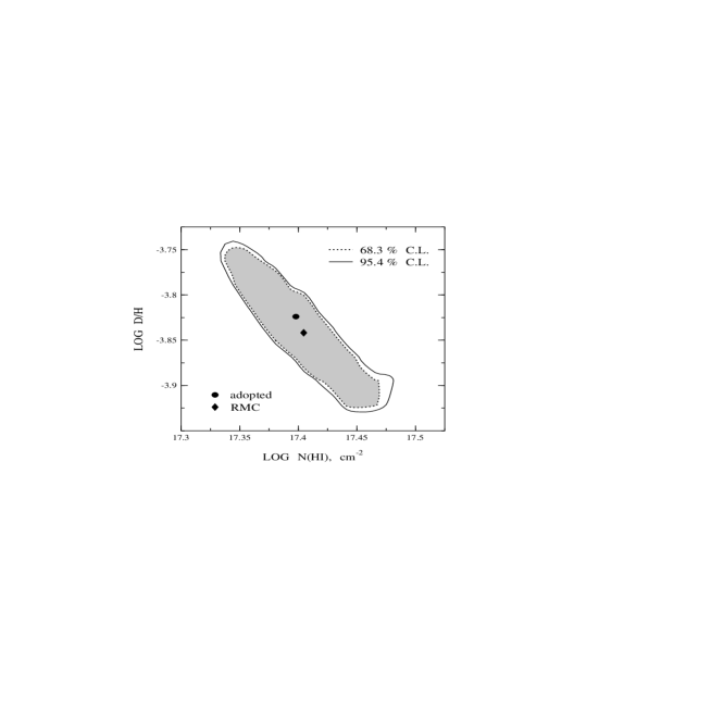
Figure 3: Confidence region for the plane ‘log N(HI) – log D/H’ for the fitted profile from Fig. 1b when the other parameters $T_{kin}$, $\sigma_{t}/v^{\rm H}_{th}$, and $L/l$ are fixed but the configuration of the velocity field is free. The adopted parameters and those found by the RMC procedure are labeled by the filled circle and diamond, respectively.

Let us turn back to Fig. 1. The thicker solid curve in panel a marks the portion of the H+D Ly$\alpha$ profile used in the minimization procedure. To run the RMC-code we sampled the intensity at evenly spaced intervals $\Delta\lambda$ and added to the $I(\lambda_{i})$ the ‘experimental’ errors which correspond to a signal-to-noise ratio S/N = 30 at the continuum level. The corresponding intensities and their uncertainties are shown in Fig. 1b by the open circles and error bars. We consider these data as being ‘observational’ intensities and apply our RMC-code to estimate the set of $n=5$ parameters { ${\theta}^{\star}_{j}$ } and the corresponding velocity field configuration { $v^{\star}_{j}$ }.

The estimated model parameters are accepted if $\chi^{2}_{min}$ is found to rank in the $\chi^{2}_{\nu,\alpha}$ distribution, i.e. $\chi^{2}_{min}\simeq 1$. The smooth curve in Fig. 1b shows one of the possible RMC solutions which gives an adequate fit with $\chi^{2}_{min}=1.188$ (cf. $\chi^{2}_{\nu,\alpha}=1.459$ for $\nu=30$ and $\alpha=0.05$). It corresponds to the model parameters $N^{\star}_{\rm HI}=2.54\times 10^{17}\ {\rm cm}^{-2}$, (D/H)${}^{\star}=1.44\times 10^{-4}$, $T^{\star}_{kin}=1216$ K, $(\sigma_{t}/v^{\rm H}_{th})^{\star}=2.02$, $(L/l)^{\star}=5.06$, and the $v^{\star}$-configuration shown in Fig. 1c by the solid curve. It is worthwhile to emphasize once more that the derived $v^{\star}$-configuration is not unique : depending on the initial condition (configuration of the velocity field) we may obtain several patterns for the velocity field distribution that satisfy our acceptance condition (each of them has its mirror counterpart which is also acceptable, of course). But the projected velocity distribution $p(u)$ has approximately the same shape for all possible RMC solutions. An example of $p(u)$ for the adopted and estimated velocity distributions is shown in Fig. 1d by the dotted and solid histograms, respectively [here $u$ means the normalized velocity $u(s)=v(s)/\sigma_{t}$].

The RMC procedure may result in the velocity field configuration becoming stuck in a local minimum of the ${\cal L}$-function for a very long period (‘meta-stable’ state). Such a minimum may not solve the required problem at all. This difficulty may be circumvented by making a few starts from different random initial configurations. Numerical experiments have shown that for a given point ${\hat{\theta}}$  the $\chi^{2}_{min}$ values may scatter by about 30 per cent around the mean due to the probabilistic character of the solution for the velocity field. This fact should be taken into account when the error surface is calculated in order to determine the confidence regions for the estimated parameters { $\theta^{\star}_{j}$ }. To get meaningful confidence limits for fitted parameters the error surface must be calculated several times with different starting points. Having calculated a set of error surfaces, the best one may be obtained by simply picking the smallest $\chi^{2}$ values for each point in the computational grid.

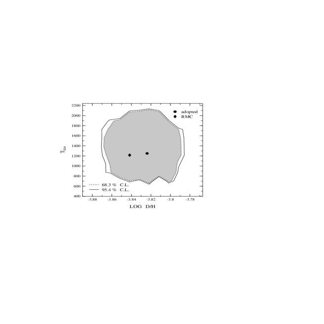
Figure 4: Confidence region for the plane ‘log D/H – $T_{kin}$’ for the fitted profile from Fig. 1b when the other parameters $N_{\rm HI}$, $\sigma_{t}/v^{\rm H}_{th}$, and $L/l$ are fixed but the configuration of the velocity field is free. The adopted parameters and those found by the RMC procedure are labeled by the filled circle and diamond, respectively.

Two examples of the confidence regions for the ‘log $N_{\rm HI}$ – log D/H’ and ‘log D/H – $T_{kin}$’ projections are presented in Fig. 3 and 4, respectively. The results were obtained from a set of six computed error surfaces for each case. Shown are two confidence ‘ellipses’ – the regions constrained by the $\chi^{2}$ values corresponding to 68.3 % and 95.4 % C.L. (1$\sigma$ and 2$\sigma$ regions for a normal distribution of residues, respectively). The RMC solutions are labeled by the filled diamonds whereas the filled circles mark the adopted quantities used to produce the ‘observed’ spectrum. A good agreement within statistical errors between these two points and between the two projected velocity field distributions can be considered as a justification of our computational procedure.

It is worth emphasizing that the elongated and declined shape of the confidence regions in Fig. 3 shows that the D/H value is strongly anti-correlated with $N_{\rm HI}$. Therefore the D/H estimates may be badly dependent on the assumed hydrogen column density.

The correlation between $T_{kin}$ and D/H is less pronounced. However, Fig. 4 shows that the kinetic temperature is not well determined in general. It seems reasonable to assume that the narrowest subcomponent of a complex absorption spectrum can show only an upper limit for $T_{kin}$ since the correlated structure of the velocity field hampers the exact measurement of $T_{kin}$ from the apparent $b$-values (see Paper II, for details).

3 Application to QSO data

The example from Subsection 2.2 demonstrates that complexity (and/or asymmetry) of an observed absorption spectrum is not necessary an indication of a clumpy structure of the absorbing material but may be solely caused by the correlations in the velocity field. Therefore one may try to explain the observed spectra starting with a minimum number of ad hoc assumptions concerning the structure of the absorber. In particular, one may consider a cloud model with a homogeneous density and temperature, assuming that the observed H+D absorption from QSO spectra arises in the outer regions (halos) of the putative intervening galaxies (cf. Tytler et al. 1996). If this is the case, then $N_{\rm HI}$ ranges from $\sim 10^{17}$ to $\sim 10^{18}$ cm^-2. This in turn means that the geometrical size of the absorbing material (parameter $L$ in our model) may be very large, $L\sim 10$ kpc. If there are many random velocity elements along the line of sight ($L/l\gg 1$), the theoretical expectation value $\langle I_{\lambda}\rangle$ should be a good approximation to the observations (Paper I). If, however, the ratio $L/l$ is not too large, deviations of $\langle I_{\lambda}\rangle$ from the observed profile (different kinds of asymmetry) are to be expected.

Modern observations of the H+D absorption at high redshift revealed two limiting D/H ratios $\sim 2\times 10^{-4}$ (e.g. Carswell et al. 1996), and $\sim 2\times 10^{-5}$ (e.g. Tytler et al. 1996). The primordial D/H ratio is shown to be very sensitive to the physical conditions that existed at the time of the Big Bang (e.g. Walker et al. 1991). D/H is expected to decrease with cosmic time due to processing of gas by stars. The theoretical uncertainties in the calculations of the primordial hydrogen isotopic ratio are rather small, the D/H value being predicted for a given baryon-photon ratio, $\eta$, with an accuracy of $\simeq 15$ % (see Sarkar 1996). Therefore, accurate measurements of the primordial D/H ratio would provide important constraints on the cosmological theories. Since these measurements are of fundamental importance to cosmology, the validity of the revealed two limiting D abundances and the reliability of the quoted errors should be thoroughly investigated.

In the following subsection we will show that accounting of the velocity field structure of the large scale gas flows may have a major impact to the D/H measurements.

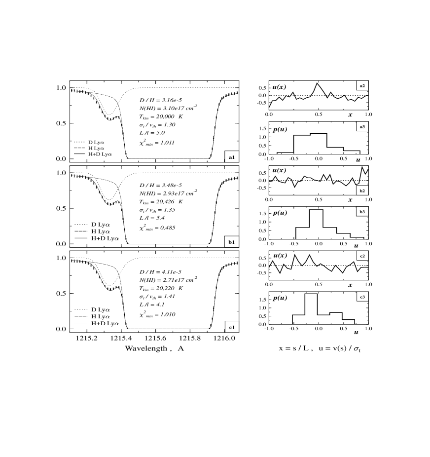
Figure 5: (a1, b1, c1) – A template H+D Ly$\alpha$ profile (dots with error bars) representing the normalized intensities and their uncertainties in accord with the B&T data. The solid curves show the results of the RMC minimization, whereas the dotted and dashed curves are the separate profiles of DI and HI, respectively. Also shown are the best fitting parameters and the $\chi^{2}$ values obtained for each case. (a2, b2, c2) – The corresponding individual realizations of the one-dimensional velocity distributions $u(x)$ in units of $\sigma_{t}$. (a3, b3, c3) – The histograms are the projected velocity distributions $p(u)$.

3.1 The $z_{a}=2.504$ system in Q 1009+2956

The RMC procedure was applied to the D absorption observed by B&T at $z_{a}=2.504$ in front of the quasar Q 1009+2956.

Using a two-cloud microturbulent model and applying a Voigt profile fitting procedure, B&T derived the following parameters for this system : total hydrogen column density $N_{\rm HI}$ = $2.9^{+0.4}_{-0.3}\times 10^{17}$ cm^-2 and D/H = $3.0^{+0.6}_{-0.5}\times 10^{-5}$; individual $T_{kin}$ = $2.1^{+0.1}_{-0.1}\times 10^{4}$ K   and $2.4^{+0.7}_{-0.7}\times 10^{4}$ K for the blue and red subcomponents, respectively, the corresponding turbulent velocities $b_{turb}=3.2\pm 0.4$ km s^-1 and $2.3\pm 1.4$ km s^-1, and a difference in the radial velocity (derived from metal lines) of 11 km s^-1. Including corrections for possible weak HI absorption at the position of D (estimated as an expected value in Monte Carlo simulations), B&T reduced the measured D/H ratio to log (D/H) = $-4.60\pm 0.08\pm 0.06$ (i.e. D/H $\simeq 2.5\times 10^{-5}$), where the $1\sigma$ random error followed by the systematic error from fitting the continuum level are given. However, for a given line of sight the proper correction is never known, and therefore we will not reduce D/H values in our analysis. This should be borne in mind when discussing the true D abundance.

We start with the calculation of a template spectrum using the parameters of B&T listed in their Table 1. To simulate real data, the experimental uncertainties are added to the computed intensities which were sampled in equidistant bins as shown in Fig. 5(a1,b1,c1) by dots and corresponding error bars. For the redshift the mean value of 2.504 was adopted and a one-component mesoturbulent model with a homogeneous density and temperature was used to construct the objective function.

Adequate profile fits ($\chi^{2}_{min}$ per degree of freedom $\la 1$) for three different sets of parameters are shown in panels (a1,b1,c1) of Fig. 5 by solid curves, whereas the individual HI and DI Ly$\alpha$ profiles are shown by dashed and dotted curves, respectively. The estimated parameters and corresponding $\chi^{2}_{min}$ values are also listed in these panels for each solution. The adjusted $u(x)$-configurations (panels a2,b2,c2) and their projected distributions $p(u)$ (panels a3,b3,c3) show pronounced deviations from a single Gaussian. Such distributions may, in principle, have very long positive ‘tails’ yielding unobservable D absorption which is hidden by the core of the hydrogen line. However, including in the objective function both the blue and the red wing of the HI line, allows to constrain significantly the set of the $u(x)$-configurations. As a result the uncertainty for the D/H measurements is considerably reduced.

In accord with our calculations, the restored profile of the DI line in the $z_{a}=2.504$ system is almost symmetrical. A slight asymmetry of the red DI Ly$\alpha$ wing is caused by the weak distortion of the $p(u)$ distribution toward positive $u$-values. In this case the width of the DI line may be formally characterized by the $b$-parameter : $b_{\rm DI}=v^{\rm D}_{th}[1+2(\sigma_{t}/v^{\rm D}_{th})^{2}]^{1/2}$ . The inspection of Fig. 5 (a1,b1,c1) reveals rather small $b_{\rm DI}$ value ($\simeq 15$ km s^-1) as compared with $\sigma_{t}\simeq 25$ km s^-1 obtained by the RMC procedure. This is not a surprise, however, because random realization of the correlated velocity field may have $p(u)$ which deviates substantially from the ensemble average distribution (assumed to be Gaussian in this case) leading to a ‘contraction’ of this distribution (see Paper II).

One may further be interested in the question whether such weak asymmetry of $p(u)$ is essential for the analysis of the H+D Ly$\alpha$ profile, or whether a simpler one component microturbulent model could be used to study the $z_{a}=2.504$ absorber. The answer is that it is essential indeed, and that the simplified model fails to reproduce the profile in question. The smallest $\chi^{2}_{min}$ value obtained for this model is only 2.4 which rejects the one-component microturbulent solution. This example clearly demonstrates once more that the analysis of absorption spectra may be very sensitive to the model assumptions concerning the velocity field structure.

The essential difference between the results of B&T and ours lies in the estimation of the hydrodynamical velocities in the $z_{a}=2.504$ absorbing region. The two-component microturbulent model yielded $b^{\rm D}_{blue}=b^{\rm D}_{red}=14$ km s^-1 and $b_{turb}\simeq 3$ km s^-1 which is about 10 times smaller than $\sqrt{2}\sigma_{t}$ estimated by the RMC procedure. For the additional parameter $L/l$ of the mesoturbulent model, we found a value of $\simeq 5$, indicating that the space averaging along the line of sight corresponds to an incomplete statistical sample and, hence, significant deviations of the observed intensities from their expectation values may occur.

As for the other parameters ($N_{\rm HI}$, D/H, and $T_{kin}$), the RMC method yields in this particular case values which are similar to those of B&T. The total hydrogen column densities and the D/H ratios obtained are shown in Fig. 6 by the filled diamond for the best RMC solution (panel b1 in Fig. 5) and by the filled circle for the B&T model (the error bars shown correspond to $1\sigma$ in accord with the B&T data from Table 1). The filled triangle and square mark the ($N_{\rm HI}$, D/H) pairs found separately for the blue and red components. The D abundance for the red component was assumed by B&T as (D/H)_red = (D/H)_blue = (D/H)_total and, thus, there was no real measurements of the D/H value for the red component in their model. This is marked by arrows instead of error bars at the filled square in Fig. 6. The projection of the 5-dimensional error surface onto the ‘log $N_{\rm HI}$ – log D/H’ plane was calculated by the RMC procedure using the $\Delta(\chi^{2})$ method. Drawn are 68 % and 95 % confidence regions computed under the condition that the parameters $T_{kin}$, $\sigma_{t}/v_{th}$, and $L/l$ are fixed, but the velocity field configuration is free. As seen, the B&T value for the total $N_{\rm HI}$ is located closely to the RMC confidence regions, but the D/H ratio is systematically lower in the microturbulent model.

Fig. 7 shows 68 % and 95 % confidence regions for the two parameters $T_{kin}$ and D/H computed under the assumption that $N_{\rm HI}$, $\sigma_{t}/v_{th}$, and $L/l$ are fixed, but the $u(x)$-configuration is free. The kinetic temperature is found in the range from $\sim 15000$ K to $\sim 22000$ K, whereas D/H lies between $\sim 3.3\times 10^{-5}$ and $\sim 4.5\times 10^{-5}$. In this figure, the filled symbols label the RMC and B&T best fitting parameters in the same sense as in Fig. 6. Note the marginal position of the RMC solution (the filled diamond) which shows that there are points in the ‘D/H – $T_{kin}$’ plane with $\chi^{2}$ values less than $\chi^{2}_{min}=0.485$ adopted for the best RMC solution at the first stage of calculations. Fig. 7 shows that also in the ‘D/H – $T_{kin}$’ plane the D/H uncertainty region is shifted toward higher D/H values as compared with the B&T data.

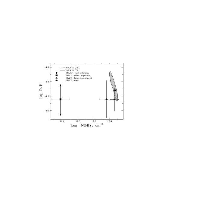
Figure 6: Confidence region for the plane ‘log N(HI) – log D/H’ for the fitted profile from Fig. 5(b1) when the other parameters $T_{kin}$, $\sigma_{t}/v^{\rm H}_{th}$, and $L/l$ are fixed but the configuration of the velocity field is free. The RMC solution is labeled by the filled diamond. The filled square and triangle represent the B&T parameters for the red and blue components of their two-component microturbulent model, and the filled circle marks the combined solution. The error bars correspond to 1$\sigma$ in accord with B&T, but the arrows reflect the fact that the D abundance was estimated through the blue component mainly and (D/H)_red = (D/H)_blue was assumed by B&T.

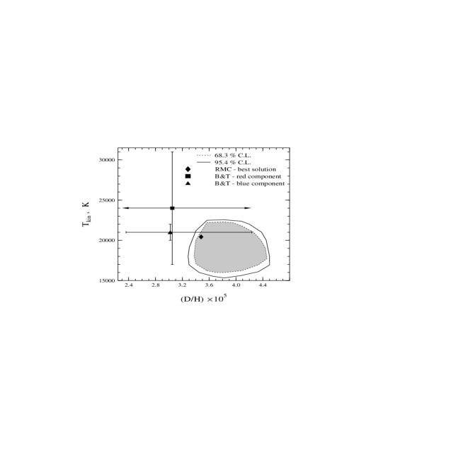
Figure 7: Confidence region for the plane ‘D/H – $T_{kin}$’ for the fitted profile from Fig. 5(b1) when the other parameters $N_{\rm HI}$, $\sigma_{t}/v^{\rm H}_{th}$, and $L/l$ are fixed but the configuration of the velocity field is free. The symbols used have the same meaning as in Fig. 6.

Above it was noted that the D/H ratio does sensitively depend on the $N_{\rm HI}$ value chosen. The measured D/H value and its confidence interval are both also affected by the choice of the velocity field configuration. The accuracy of the RMC solution may be increased if some additional information about the velocity field structure is available for the analysis. For instance, the profile shapes of higher order Lyman lines may yield additional useful constraints to the allowable $p(u)$ distribution. For this case the size of the D/H uncertainty interval may be narrowed down. This is demonstrated in Fig. 8 where the results of two calculations (formally called ‘high’ and ‘low’ D/H) are shown. The 68 % and 95 % confidence regions were computed for the fixed $T_{kin}$, $\sigma_{t}/v_{th}$, and $L/l$ listed in panels c1 and a1 (Fig. 5), respectively, and for the fixed configurations of $u(x)$ shown in panels c2 and a2 (Fig. 5). Provided the constraints mentioned above are available and, thus a distinction between different $p(u)$ distributions compatible with the measured H+D profile (Fig. 5) is possible, the accuracy of the D/H measurements improves essentially becoming comparable with the accuracy of the SBBN calculations (Sarkar 1996).

We now discuss the observed D abundance and its inferred primordial value which can be compared with the SBBN model predictions. Within the framework of the SBBN, the primordial abundances of the light elements (D, ³He, ⁴He, ⁷Li) depend only on the baryon to photon ratio $\eta=n_{b}/n_{\gamma}$, where $n_{b}$ is the current cosmological number density of baryons and $n_{\gamma}$ is the number density of the cosmic background photons. The predicted relations between the abundances of D, ⁴He, and ⁷Li and $\eta$ are illustrated in Fig. 9. The thick solid curves plotted in this figure are computed by using the analytical formulae from Sarkar (1996), while dashed curves depict their uncertainty intervals. The primordial mass fraction of ⁴He, $Y_{p}=0.243\pm 0.003$, was derived by Izotov et al. (1997), and Bonifacio & Molaro (1997) give the following value for the lithium abundance in halo population II stars : log (⁷Li/H)${}_{p}^{\rm II}$ = $-9.762\pm 0.012\pm 0.05$ (here the subscript p denotes primordial). The uncertainty regions for the measured values of Y${}_{p}({}^{4}$He) and (⁷Li/H)${}_{p}^{\rm II}$ and the implied SBBN limits on $\eta$ are shown by the solid-line rectangles in Fig. 9(b,c). The upper panel a in this figure gives our results : the solid-line rectangle is defined by the 95 % confidence region (shown in Fig. 6) for an arbitrary configuration of the velocity field, whereas two dotted-line rectangles correspond to 68 % confidence regions computed for the two fixed velocity fields leading to the ‘high D/H’ and ‘low D/H’ solutions shown in Fig. 8. The shaded region in Fig. 9 represents the range of $\eta$ compatible with the measured abundances of all three nuclei. Fig. 9 shows that concordance of D/H with Y${}_{p}({}^{4}$He) and (⁷Li/H)${}_{p}^{\rm II}$ measurements is achieved if $3.9\times 10^{-10}\la\eta\la 5.3\times 10^{-10}$. This constraint on $\eta$ is consistent with results of other groups; for example, Hata et al. (1995) quote $\eta=4.4^{+0.8}_{-0.6}\times 10^{-10}$ $(1\sigma)$ [see also Sarkar (1996) for a discussion of the intercomparisons of the allowed $\eta$-intervals]. The center of the shaded $\eta$-interval in Fig. 9 corresponds to $\Omega_{b}h^{2}=0.017$, where $\Omega_{b}$ is the fraction of the critical density contributed by baryons and $h$ the Hubble constant in units 100 km s^-1 Mpc^-1. The uncertainties in this estimation can alter $\Omega_{b}$ by up to $\simeq 20$ %.

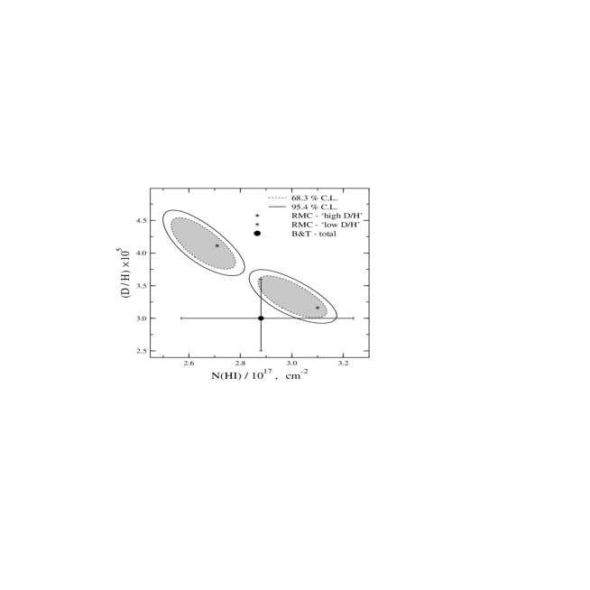
Figure 8: Confidence region for the plane ‘N(HI) – D/H’ for the fitted profiles from Fig. 5 a1 and c1 when the other parameters $T_{kin}$, $\sigma_{t}/v^{\rm H}_{th}$, and $L/l$ and the corresponding configurations of the velocity fields (shown in Fig. 5 a2, c2) are fixed. The RMC ‘high D/H’ and ‘low D/H’ solutions are labeled by star and asterisk, respectively. The filled circle and 1$\sigma$ error bars represent the B&T result.

4 Conclusions

The origin of QSO absorption-line systems with HI column densities $\sim 10^{17}-10^{18}$ cm^-2 (which are particularly useful for deuterium observations) is usually associated with extended gas halos of foreground galaxies. According to recent high resolution observations, the line profiles in these systems are often wider than expected from purely thermal broadening, and, therefore, their widths reflect both thermal and turbulent broadening caused by any kind of bulk motions in the halos. In turbulent media the determination of HI and DI column densities depends on the model (micro- or mesoturbulent) is chosen for the profile analysis. The microturbulent model yields reasonable results if $\sigma_{t}\ll v_{th}$ , or $L/l\gg 1$, otherwise the mesoturbulent one is more adequate.

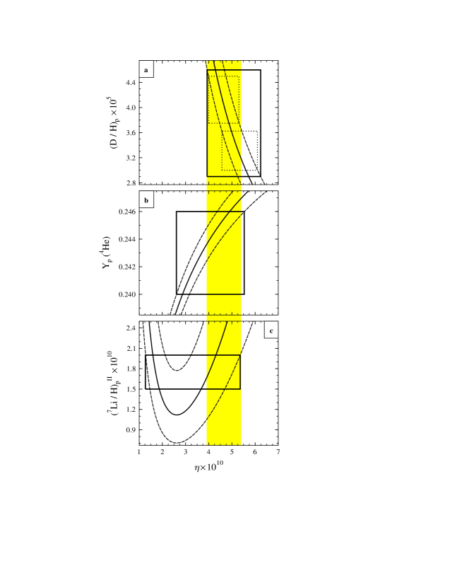
Figure 9: Comparison of predicted primordial abundances (denoted by the subscript p) with observational bounds. The theoretical SBBN  D, ⁴He, and ⁷Li yields (solid curves) and their uncertainties (dashed curves) as function of $\eta$ (the baryon to photon number ratio) are computed by using the parameterization of Sarkar (1996). The abundances of D and ⁷Li are number ratios, whereas Y_p is the mass fraction of ⁴He. The hight of the solid-line rectangles in panels b and c give the bounds from recent measurements of extra-galactic Y_p (Izotov et al. 1997) and ⁷Li in population II (halo) stars (Bonifacio & Molaro 1997). The horizontal widths give the range of $\eta$ compatible with the measurements. In panel a the solid-line rectangle corresponds to the 2$\sigma$ uncertainty region for D/H towards Q1009+2956, as calculated by the RMC procedure for an arbitrary velocity field configuration (see Fig. 6), whereas the two dotted-line rectangles are defined by the 68 % confidence regions shown in Fig. 8 (the velocity field structure is fixed). The shaded region is the window for $\eta$ common to all results.

Direct observations of the Ly$\alpha$ emission of distant galaxies ($z>2$) show that their giant halos ($R\sim 100$ kpc) have complex morphologies and kinematics (Röttgering et al. 1996). The observations reveal as well extended HI absorption systems (with projected sizes up to $\sim 50$ kpc) seen against the Ly$\alpha$ emission (van Ojik et al. 1997).

Using the measured Doppler parameters for the absorbing gas with $N_{\rm HI}\simeq 10^{18.1}-10^{18.5}$ cm^-2 (see Table 3 in van Ojik et al.) and the kinetic temperature $T_{kin}=10^{4}$ K adopted by van Ojik et al., we can estimate the range for the velocity dispersion of bulk motions : 24 km s${}^{-1}\la\sigma_{t}\la 55$ km s^-1. It follows that $\sigma_{t}/v_{th}>1$ within the HI absorption line gas embedded in the galactic halos. Both findings – high absolute value of $\sigma_{t}$ and high $\sigma_{t}/v_{th}$ ratio, – make the mesoturbulent approach to appear to be more realistic one. Besides, our present RMC calculations yielded for the $z_{a}=2.504$ absorption system $\sigma_{t}\simeq 25$ km s^-1 which lies just within the observed range, whereas $\sigma_{t}\simeq 2$ km s^-1 found by B&T is evidently too low.

The main conclusion of our work is that the mesoturbulent approach together with the RMC computational scheme allows to solve the inverse problem for the H+D Ly$\alpha$ absorption and to restore the physical parameters of the absorbing gas as well as the projection of the velocity field distribution.

The proposed computational procedure enables us to draw confidence regions for different pairs of the adopted parameters. From the analysis of the synthetic H+D Ly$\alpha$ spectrum it was found that, in general, the measured D/H and $N_{\rm HI}$ values are anti-correlated.

The study of the template H+D Ly$\alpha$ profile (which reproduces the original spectrum of B&T) yields D/H = $(3.75\pm 0.85)\times 10^{-5}$ $(2\sigma)$. We therefore adopt the value of $4.6\times 10^{-5}$ as a conservative upper limit on the primordial abundance of D relative to hydrogen.

We conclude that the discordance of D/H with the ⁴He and ⁷Li primordial abundances noted by B&T is a consequence of the use of the microturbulent model. Within the framework of the generalized model one finds good agreement between the measurements mentioned above and the SBBN predictions.

Acknowledgments

This work was supported by the Deutsche Forschungsgemeinschaft, and by the RFBR grant No. 96-02-16905-a. The authors thank Dr. I. Agafonova for valuable suggestions on the RMC technique and for her kind help in the development of the RMC computer code. SAL gratefully acknowledges the hospitality of the Institut für Theoretische Physik der Universität Frankfurt am Main.

References

- [Bonifacio & Molaro1997] Bonifacio P., Molaro P., 1997, MNRAS, 285, 847
- [Burles & Tytler1996] Burles S., Tytler D., 1996, Science, submitted, astro-ph 9603070
- [Carswell et al.1994] Carswell R. F., Webb J. K., Lanzetta K. M., Baldwin J. A., Cooke A. J., Williger G. M., Rauch M., Irwin M. J., Robertson J. G., Shaver P. A., 1996, MNRAS, 278, 506
- [Frye et al.1997] Frye B., Welch W. J., Broadhurst T., 1997, ApJ, L25
- [Hata et al.1995] Hata N., Scherrer R. J., Steigman G., Thomas D., Walker T. P., Bludman S., Langacker P., 1995, Phys. Rev. Lett., 75, 3977
- [Hoffmann1995] Hoffmann K. H., 1995, in Computational Physics, eds. K. H. Hoffmann, M. Schreiber (Springer : Berlin), p.45
- [Izotov et al.1997] Izotov Yu., Thuan T. X., Lipovetsky V. A., 1997, ApJS, 108, 1
- [Levshakov & Kegel1994] Levshakov S. A., Kegel W. H., 1994, MNRAS, 271, 161
- [Levshakov & Kegel1996] Levshakov S. A., Kegel W. H., 1996, MNRAS, 278, 497
- [Levshakov & Takahara1996a] Levshakov S. A., Takahara F., 1996a, MNRAS, 279, 651
- [Levshakov & Takahara1996b] Levshakov S. A., Takahara F., 1996b, Astron. Lett., 22, 438
- [Levshakov & Kegel1997] Levshakov S. A., Kegel W. H., 1997, MNRAS, 288, 787, (Paper I)
- [Levshakov et al.1997] Levshakov S. A., Kegel W. H., Mazets I. E., 1997, MNRAS, 288, 802, (Paper II)
- [Linsky et al.1995] Linsky J. L., Diplas A., Wood B. E., Brown A., Ayres T. R., Savage B D., 1995, ApJ, 451, 335
- [Metropolis et al.1953] Metropolis N., Rosenbluth A. W., Rosenbluth M. N., Teller A. H., Teller E., 1953, J. Chem. Phys., 21, 1087
- [Press et al.1953] Press W. H., Teukolsky S. A., Vetterling W. T., Flannery B. P., 1992, Numerical Recipes in C (Cambridge University Press : Cambridge), p.444
- [Röttgering et al.1996] Röttgering H., Miley G., van Ojik R., 1996, The Messenger, 83, 26
- [Sarkar1996] Sarkar S., 1996, Rep. Prog. Phys., 59, 1493
- [Tytler et al.1996] Tytler D., Fan X.-M., Burles S., 1996, Nat, 381, 207
- [van Ojik et al.1997] van Ojik R., Röttgering H. J. A., Miley G. K., Hunstead R. W., 1997, A&A, 317, 358
- [Walker et al.1991] Walker T. P., Steigman G., Schramm D. N., Olive K. A., Kang H.-S., 1991, ApJ, 376, 51