Correlation Functions of CMB Anisotropy and Polarization

Abstract

We give a full analysis of the auto- and cross-correlations between the Stokes parameters of the cosmic microwave background. In particular, we derive the windowing function for an antenna with Gaussian response in polarization experiment, and construct correlation function estimators corrected for instrumental noise. They are applied to calculate the signal to noise ratios for future anisotropy and polarization measurements. While the small-angular-scale anisotropy-polarization correlation would be likely detected by the MAP satellite, the detection of electric and magnetic polarization would require higher experimental sensitivity. For large-angular-scale measurements such as the being planned SPOrt/ISS, the expected signal to noise ratio for polarization is greater than one only for reionized models with high reionization redshifts, and the ratio is less for anisotropy-polarization correlation. Correlation and covariance matrices for likelihood analyses of ground-based and satellite data are also given.

I Introduction

The detection of the large-angle anisotropy of the cosmic microwave background (CMB) by the COBE DMR experiment [1] provided important evidence of large-scale spacetime inhomogenities. Since then, a dozen of small-scale anisotropy measurements have hinted that the Doppler peak resulting from acoustic oscillations of the baryon-photon plasma on the last scattering surface seems to be present [2]. CMB measurements gain an advantage over other traditional observations due to the fact that the small CMB fluctuations can be well treated as linear, while the low-redshift universe is in a non-linear regime. It is now well established that CMB temperature anisotropies are genuine imprint of the early universe, which could potentially be used to determine to a high precision virtually all cosmological parameters of interest. It has been estimated that a number of cosmological parameters can be determined with standard errors of $10\%$ or better by the upcoming NASA MAP satellite [3]. Furthermore, the future Planck Surveyor CMB mission would have capability of observing the early universe about 100 times better than MAP.

At this point, we should explore as much information as possible besides the temperature anisotropy contained in the relic photons. Anisotropic radiation possessing a non-zero quadrupole moment acquires a net linear polarization when it is scattered with electrons via Thomson scattering [4] (also see Eq. (6) of Ref. [5]). When the photons begin to decouple from the matter on the last scattering surface and develope a quadrupole anisotropy via Sachs-Wolfe effect [6], linear polarization is created from scatterings with free electrons near the last scattering surface. Studies have shown that on small angular scales the rms polarization, in a standard universe, is a few percents of the rms anisotropy, while the large-scale polarization is insignificant [7]. In models with early reionization, the large-scale polarization is greatly enhanced, to a few percents level, but the small-scale anisotropy is suppressed significantly [5, 8]. Therefore, CMB polarization would provide a valuable complementary information to the anisotropy measurements. In addition, the anisotropy-polarization cross correlation offers a test of physics on the last scattering surface, as well as a possibility of distinguishing the scalar and tensor perturbations [9, 10]. However, all of these polarization calculations have relied on a small-angle approximation, which may not be valid when a large sky-coverage is considered.

As such, full-sky analyses of the polarization have been performed  [11, 12, 13, 14, 15]. It was found that there are modifications to low multipole moments ($l<30$) of the polarization power spectra, where the tensor contribution dominates over the scalar contribution [11, 14]. More importantly, rotationally invariant power spectra of the Stokes parameters have been constructed [12, 13, 14, 15]. In particular, one of them is a parity-odd magnetic polarization spectrum, which vanishes for scalar-induced polarization, thereby allowing one to make a model-independent identification of non-scalar (i.e. vector or tensor) perturbations (also see Ref. [16]). Recently it was shown that magnetic polarization would be a strong discriminator between defect and inflation models [17, 18]. Also, a new physically transparent formalism based on the total angular momentum representation [19] was proposed [17, 20], which simplifies the radiative transport problem and can be easily generalized to open universes [21].

Since polarization fluctuations are typically at a part in a million, an order magnitude below the temperature fluctuations, to measure this signal requires high detector sensitivity, long integration time, and/or a large number of pixels. So far, only experimental upper limits have been obtained [22, 23, 24], with the current limit on the linear polarization being $16\mu K$ [24]. Ground-based experiments being planned or built will probably achieve detection sensitivity using low-noise HEMT amplifiers as well as long hours of integration time per pixel. The MAP satellite will launch in 2000 and make polarization measurements of the whole sky in about $10^{5}$ pixels. If the polarization foreground can be successfully removed, MAP should marginally reach the detection level. For a detection of the magnetic polarization one would require either several years of MAP observations or the Planck mission [12, 18, 25]. We expect that polarization measurements are as important as anisotropy in future missions.

Previous full-sky studies of the polarization are mainly based on angular power spectrum estimators in Fourier space. Although electric- and magnetic-type scalar fields $E$ and $B$ in real space can be constructed, they must involve nonlocal derivatives of the Stokes components. In this paper, we will study in detail the auto- and cross-correlation functions of the Stokes parameters themselves in real space. Although the two approaches should be equivalent to each other, one can find individual advantages in different situations. We will follow the formalism of Ref. [12], expanding the Stokes parameters in terms of spin-weighted spherical harmonics. The expansion coefficients are rotationally invariant power spectra which will be evaluated using CMBFAST Boltzmann code developed by Seljak and Zaldarriaga [26]. In Sec. II we briefly introduce the CMB Stokes parameters and their relation to spin-weighted spherical harmonics. Sec. III is devoted to discussions of the properties of the harmonics, the harmonics representation of rotation group, and the generalized addition theorem and recursion relation. In Sec. IV we expand the Stokes parameters in spin-weighted harmonics, and briefly explain how to compute the power spectra induced by scalar and tensor perturbations. In Sec. V we derive window functions appropriate to detectors with Gaussian angular response in anisotropy and polarization experiments. The instrumental noise of detectors in CMB measurements is treated in Sec. VI as white noise superposed upon the microwave sky. Sec. VII is to construct the auto- and cross-correlation function estimators corrected for noise bias in terms of the power spectra. As examples, in Sec. VIII we compute the means and variances of the estimators for different configurations of future space missions in standard cold dark matter models. Further, we outline the likelihood analysis of the experimental data in Sec. IX. Sec. X is our conclusions.

II Stokes Parameters

Polarized light is conventionally described in terms of the four Stokes parameters $(I,Q,U,V)$, where $I$ is the intensity, $Q$ and $U$ represent the linear polarization, and $V$ describes the circular polarization. Each parameter is a function of the photon propogation direction $\hat{n}$. Let us define

$$T=I-{\bar{I}}$$ (1)

as the temperature fluctuation about the mean. Since circular polarization cannot be generated by Thomson scattering alone, $V$ decouples from the other components. So, it suffices to consider only the Stokes components $(T,Q,U)$ as far as CMB anisotropy and polarization is concerned. Traditionally, for radiation propagating radially along $\hat{e}_{r}$ in the spherical coordinate system, see Fig. 1, $Q$ and $U$ are defined with respect to an orthonormal basis $(\hat{a},\hat{b})$ on the sphere, which are related to $(\hat{e}_{\theta},\hat{e}_{\phi})$ by

$$\hat{a}=\hat{e}_{\phi},\quad{\rm and}\quad\hat{b}=-\hat{e}_{\theta}.$$ (2)

Then, $Q$ is the difference in intensity polarized in the $\hat{b}$ and $\hat{a}$ directions, while $U$ is the difference in the $(\hat{a}+\hat{b})/\sqrt{2}$ and $(\hat{a}-\hat{b})/\sqrt{2}$ directions [27]. Under a left-handed rotation of the basis about $\hat{e}_{r}$ through an angle $\psi$,

$$\left(\begin{array}[]{c}\hat{a}^{\prime}\\ \hat{b}^{\prime}\end{array}\right)=\left(\begin{array}[]{cc}\cos\psi&-\sin\psi\\ \sin\psi&\cos\psi\end{array}\right)\left(\begin{array}[]{c}\hat{a}\\ \hat{b}\end{array}\right),$$ (3)

or equivalently,

$$\frac{1}{\sqrt{2}}\left(\hat{a}^{\prime}+i\hat{b}^{\prime}\right)=e^{i\psi}\frac{1}{\sqrt{2}}\left(\hat{a}+i\hat{b}\right).$$ (4)

Under this transformation $T$ and $V$ are invariant while $Q$ and $U$ being transformed to [27]

$$\left(\begin{array}[]{c}Q^{\prime}\\ U^{\prime}\end{array}\right)=\left(\begin{array}[]{cc}\cos 2\psi&\sin 2\psi\\ -\sin 2\psi&\cos 2\psi\end{array}\right)\left(\begin{array}[]{c}Q\\ U\end{array}\right),$$ (5)

which in complex form is

$$Q^{\prime}(\hat{e}_{r})\pm iU^{\prime}(\hat{e}_{r})=e^{\mp 2i\psi}\left[Q(\hat{e}_{r})\pm iU(\hat{e}_{r})\right].$$ (6)

Hence, $Q(\hat{n})\pm iU(\hat{n})$ has spin-weight $\mp 2$. Therefore, we may expand each Stokes parameter in its appropriate spin-weighted spherical harmonics [19, 12].

Unfortunately, the convention in theory has a little difference from experimental practice. In CMB polarization measurements, usually the north celestial pole is chosen as the reference axis $\hat{e}_{3}$, and linear polarization at a point $\hat{x}$ on the celestial sphere is defined by

$${\cal Q}(\hat{x})=T_{N,S}-T_{E,W},\quad{\rm and}\quad{\cal U}(\hat{x})=T_{NE,SW}-T_{NW,SE},$$ (7)

where $T_{N,S}$ is the antenna temperature of radiation polarized along the north-south direction, and so on [22]. In small-scale experiments covering only small patches of the sky, the geometry is essentially flat, so one can simply choose any local rectangular coordinates to define ${\cal Q}$ and ${\cal U}$. Since an observation in direction $\hat{x}$ receives radiation with propagating direction $\hat{n}=-\hat{x}$, we have

$${\cal Q}(\hat{x})=Q(\hat{n}),\quad{\rm and}\quad{\cal U}(\hat{x})=-U(\hat{n}).$$ (8)

III Spin-weighted Spherical Harmonics

An explicit expression of spin-$s$ spherical harmonics is  [28, 29]

$$\>{}_{s}Y_{lm}(\theta,\phi) =(-1)^{m}e^{im\phi}\left[\frac{2l+1}{4\pi}\frac{(l+m)!}{(l+s)!}\frac{(l-m)!}{(l-s)!}\right]^{\frac{1}{2}}\sin^{2l}\left(\frac{\theta}{2}\right)$$ (14)

$$\times\sum_{r}\left(\begin{array}[]{c}l-s\\ r\\ \end{array}\right)\left(\begin{array}[]{c}l+s\\ r+s-m\\ \end{array}\right)(-1)^{l-s-r}\cot^{2r+s-m}\left(\frac{\theta}{2}\right),$$

where

$$\max(0,m-s)\leq r\leq\min(l-s,l+m).$$ (15)

Note that the common spherical harmonics $Y_{lm}=\>_{0}Y_{lm}$. They have the conjugation relation and parity relation:

$$\>{}_{s}Y^{*}_{lm}(\theta,\phi)=(-1)^{m+s}\>_{-s}Y_{l-m}(\theta,\phi),$$ (16)

$$\>{}_{s}Y_{lm}(\pi-\theta,\phi+\pi)=(-1)^{l}\>_{-s}Y_{lm}(\theta,\phi).$$ (17)

They satisfy the orthonormality condition and completeness relation:

$$\int d\Omega\>_{s}Y^{*}_{l^{\prime}m^{\prime}}(\theta,\phi)\>_{s}Y_{lm}(\theta,\phi)=\delta_{l^{\prime}l}\delta_{m^{\prime}m},$$ (18)

$$\sum_{lm}\>{}_{s}Y^{*}_{lm}(\theta^{\prime},\phi^{\prime})\>_{s}Y_{lm}(\theta,\phi)=\delta(\phi^{\prime}-\phi)\delta(\cos\theta^{\prime}-\cos\theta).$$ (19)

Therefore, a quantity $\eta$ of spin-weight $s$ defined on the sphere can be expanded in spin-$s$ basis,

$$\eta(\theta,\phi)=\sum_{lm}\eta_{lm}\>{}_{s}Y_{lm}(\theta,\phi),$$ (20)

where the expansion coefficients $\eta_{lm}$ are scalars.

The raising and lowering operators, $\partial\!\!^{\prime}$ and $\bar{\partial\!\!^{\prime}}$, acting on $\eta$ of spin-weight $s$, are defined by [28]

$${\partial\!\!^{\prime}}\eta = -(\sin\theta)^{s}\left[\frac{\partial}{\partial\theta}+i\csc\theta\frac{\partial}{\partial\phi}\right](\sin\theta)^{-s}\eta,$$ (21)

$$\bar{\partial\!\!^{\prime}}\eta = -(\sin\theta)^{-s}\left[\frac{\partial}{\partial\theta}-i\csc\theta\frac{\partial}{\partial\phi}\right](\sin\theta)^{s}\eta.$$ (22)

When they act on the spin-$s$ spherical harmonics, we have [28]

$${\partial\!\!^{\prime}}\>_{s}Y_{lm} = \left[(l-s)(l+s+1)\right]^{1\over 2}\>_{s+1}Y_{lm},$$ (23)

$$\bar{\partial\!\!^{\prime}}\>_{s}Y_{lm} = -\left[(l+s)(l-s+1)\right]^{1\over 2}\>_{s-1}Y_{lm},$$ (24)

$$\bar{\partial\!\!^{\prime}}{\partial\!\!^{\prime}}\>_{s}Y_{lm} = -(l-s)(l+s+1)\>_{s}Y_{lm}.$$ (25)

Using these raising and lowering operations, we obtain the generalized recursion relation for $l-2\geq\max(|s|,|m|)$,

$$\left(\frac{l+s}{l-s}\right)^{1\over 2} \>{}_{s}Y_{lm}=\left[\frac{(2l+1)(2l-1)}{(l+m)(l-m)}\right]^{1\over 2}\cos\theta\>_{s}Y_{l-1,m}$$ (28)

$$-\left[\frac{(2l+1)(l+m-1)(l-m-1)(l-s-1)}{(2l-3)(l+m)(l-m)(l+s-1)}\right]^{1\over 2}\>_{s}Y_{l-2,m}$$

$$+s\left[\frac{(2l+1)(2l-1)}{(l+m)(l-m)(l-s)(l+s-1)}\right]^{1\over 2}\sin\theta\>_{s-1}Y_{l-1,m}.$$

This will be used for evaluating the correlation functions in Sec. VIII. Table 1 lists explicit expressions for some low-$l$ spin-weighted harmonics, from which higher-$l$ ones can be constructed.

The harmonics are related to the representation matrices of the 3-dimensional rotation group. If we define a rotation $R(\alpha,\beta,\gamma)$ as being composed of a rotation $\alpha$ around $\hat{e}_{3}$, followed by $\beta$ around the new $\hat{e}_{2}^{\prime}$ and finally $\gamma$ around $\hat{e}_{3}^{\prime\prime}$, the rotation matrix of $R$ will be given by [28]

$$D_{-sm}^{l}(\alpha,\beta,\gamma)=\sqrt{\frac{4\pi}{2l+1}}\>_{s}Y_{lm}(\beta,\alpha)e^{-is\gamma}.$$ (29)

Let us consider a rotation group multiplication,

$$R(\alpha,\beta,-\gamma)=R(\phi^{\prime},\theta^{\prime},0)R^{-1}(\phi,\theta,0),$$ (30)

where the angles are defined in Fig. 1. In terms of rotation matrices, it becomes

$$D^{l}_{s_{1}s_{2}}(\alpha,\beta,-\gamma)=\sum_{m}D^{l}_{s_{1}m}(\phi^{\prime},\theta^{\prime},0)D^{l*}_{s_{2}m}(\phi,\theta,0),$$ (31)

which leads to the generalized addition theorem,

$$\sum_{m}\>{}_{s_{1}}Y^{*}_{lm}(\theta^{\prime},\phi^{\prime})\>_{s_{2}}Y_{lm}(\theta,\phi)=\sqrt{\frac{2l+1}{4\pi}}(-1)^{s_{1}-s_{2}}\>_{-s_{1}}Y_{ls_{2}}(\beta,\alpha)e^{-is_{1}\gamma}.$$ (32)

IV Power Spectra

Following the notations in Ref. [12], we expand the Stokes parameters as

$$T(\hat{n}) = \sum_{lm}a_{T,lm}Y_{lm}(\hat{n}),$$ (33)

$$Q(\hat{n})-iU(\hat{n}) = \sum_{lm}a_{2,lm}\>{}_{2}Y_{lm}(\hat{n}),$$ (34)

$$Q(\hat{n})+iU(\hat{n}) = \sum_{lm}a_{-2,lm}\>{}_{-2}Y_{lm}(\hat{n}).$$ (35)

The conjugation relation (16) requires that

$$a_{T,lm}^{*}=(-1)^{m}a_{T,l-m},\quad a_{-2,lm}^{*}=(-1)^{m}a_{2,l-m}.$$ (36)

For Stokes parameters in CMB measurements, using the parity relation (17), we have

$${\cal T}(\hat{x}) = \sum_{lm}(-1)^{l}a_{T,lm}Y_{lm}(\hat{x}),$$ (37)

$${\cal Q}(\hat{x})+i{\cal U}(\hat{x}) = \sum_{lm}(-1)^{l}a_{2,lm}\>{}_{-2}Y_{lm}(\hat{x}),$$ (38)

$${\cal Q}(\hat{x})-i{\cal U}(\hat{x}) = \sum_{lm}(-1)^{l}a_{-2,lm}\>{}_{2}Y_{lm}(\hat{x}).$$ (39)

Isotropy in the mean guarantees the following ensemble averages:

$$\left<a^{*}_{T,l^{\prime}m^{\prime}}a_{T,lm}\right> = C_{Tl}\delta_{l^{\prime}l}\delta_{m^{\prime}m},$$ (40)

$$\left<a^{*}_{2,l^{\prime}m^{\prime}}a_{2,lm}\right> = (C_{El}+C_{Bl})\delta_{l^{\prime}l}\delta_{m^{\prime}m},$$ (41)

$$\left<a^{*}_{2,l^{\prime}m^{\prime}}a_{-2,lm}\right> = (C_{El}-C_{Bl})\delta_{l^{\prime}l}\delta_{m^{\prime}m},$$ (42)

$$\left<a^{*}_{T,l^{\prime}m^{\prime}}a_{2,lm}\right> = -C_{Cl}\delta_{l^{\prime}l}\delta_{m^{\prime}m}.$$ (43)

Consider two points $\hat{n}^{\prime}(\theta^{\prime},\phi^{\prime})$ and $\hat{n}(\theta,\phi)$ on the sphere. Using the addition theorem (32) and Eq. (43), we obtain the correlation functions,

$$\left<T^{*}(\hat{n}^{\prime})T(\hat{n})\right>=\sum_{l}\frac{2l+1}{4\pi}C_{Tl}P_{l}(\cos\beta),$$ (44)

$$\left<T^{*}(\hat{n}^{\prime})[Q(\hat{n})+iU(\hat{n})]\right>=-\sum_{l}\frac{2l+1}{4\pi}\sqrt{\frac{(l-2)!}{(l+2)!}}C_{Cl}P^{2}_{l}(\cos\beta)e^{2i\alpha},$$ (45)

$$\left<[Q(\hat{n}^{\prime})+iU(\hat{n}^{\prime})]^{*}[Q(\hat{n})+iU(\hat{n})]\right>=\sum_{l}\sqrt{\frac{2l+1}{4\pi}}(C_{El}+C_{Bl})\>_{2}Y_{l-2}(\beta,0)e^{2i(\alpha-\gamma)},$$ (46)

$$\left<[Q(\hat{n}^{\prime})-iU(\hat{n}^{\prime})]^{*}[Q(\hat{n})+iU(\hat{n})]\right>=\sum_{l}\sqrt{\frac{2l+1}{4\pi}}(C_{El}-C_{Bl})\>_{2}Y_{l2}(\beta,0)e^{2i(\alpha+\gamma)},$$ (47)

where $\alpha$, $\beta$, and $\gamma$ are the angles defined in Fig. 1. Eq. (45) is the most general form of those found in Refs. [9, 11, 16, 30]. In the small-angle approximation, i.e. $\beta<<1$, $\alpha\simeq\gamma$, so Eq. (46) depends only on the separation angle $\beta$. When $\hat{n}^{\prime}$ and $\hat{n}$ lie on the same longitude, $\alpha=\gamma=0$ and hence Eqs. (45,46,47) depend only on $\beta$. When $\hat{n}^{\prime}$ and $\hat{n}$ lie on the same latitude, $\alpha+\gamma=\pi$. Hence the phase angle in Eq. (47) vanishes, and that in Eq. (46) becomes equal to $e^{4i\alpha}$.

A coordinate-independent set of correlation functions has been obtained by defining correlation functions of Stokes parameters $(Q_{r},U_{r})$ with respect to axes which are parallel and perpendicular to the great arc connecting the two points being correlated [15]. This prescription is indeed equivalent to the transformations:

$$Q_{r}(\hat{n}^{\prime})+iU_{r}(\hat{n}^{\prime}) = e^{-2i\gamma}[Q(\hat{n}^{\prime})+iU(\hat{n}^{\prime})],$$ (48)

$$Q_{r}(\hat{n})+iU_{r}(\hat{n}) = e^{-2i\alpha}[Q(\hat{n})+iU(\hat{n})].$$ (49)

The authors in Ref. [15] expanded $Q_{r}$ and $U_{r}$ in terms of tensor spherical harmonics. To calculate the two-point correlation functions between $T$, $Q_{r}$, and $U_{r}$, they chose one point to be at the north pole and the other on the $\phi=0$ longitude, and argued that the correlation functions depend only on the angular separation of the two points. Then, they had to evaluate the asymptotic forms for the tensor spherical harmonics at the north pole. Their results are simply equal to the above correlation functions without the phase angles. Here, using the compact generalized addition theorem (32), we have given a general and straightforward way of obtaining the correlation functions. In addition, the phase information is retained. We will see in Sec. VII and Sec. IX that these phase angles can be easily removed or evaluated in taking experimental data.

Therefore, the statistics of the CMB anisotropy and polarization is fully described by four independent power spectra $(C_{Tl},C_{El},C_{Bl},C_{Cl})$ or their corresponding correlation functions. Here, we outline how to evaluate the spectra. The details can be found in Refs. [14, 15].

Since the four spectra are rotationally invariant, it suffices to consider the contribution from a single $\hat{k}$-mode of the perturbation, and then integrate over all the modes. In particular, the calculation will be greatly simplified if we choose $\hat{k}=\hat{e}_{3}$. For scalar perturbations, the contribution of the $\hat{k}$-mode to $(T(\hat{n}),Q(\hat{n}),U(\hat{n}))$ is $(\Delta^{(S)}_{T},\Delta^{(S)}_{P},0)$. For tensor perturbations, the contribution is

$$\left(\begin{array}[]{c}(1-\cos^{2}\theta)\cos 2\phi\,\Delta^{(T)}_{T}\\ (1+\cos^{2}\theta)\cos 2\phi\,\Delta^{(T)}_{P}\\ 2\cos\theta\sin 2\phi\,\Delta^{(T)}_{P}\end{array}\right),$$ (50)

for $+$-mode. The $\times$-mode contribution is from making the replacements, $\cos 2\phi\to\sin 2\phi$ and $\sin 2\phi\to-\cos 2\phi$. The quantities $\Delta$’s are then computed by solving the Boltzmann hierarchy equations or by the line-of-sight integration method [26]. In the following sections, we will use CMBFAST Boltzmann code [26] to evaluate all $C_{Xl}$’s.

V Window Function

Due to the finite beam size of the antenna, any information on angular scales less than about the beam width is smeared out. This effect can be approximated by a Gaussian response function,

$$dR(\beta,\alpha)=\frac{\beta\,d\beta\,d\alpha}{2\pi\sigma_{b}^{2}}\;e^{-\frac{\beta^{2}}{2\sigma_{b}^{2}}},$$ (51)

where $\sigma_{b}$, much less than $1$, is the Gaussian beam width of the antenna, $\beta$ and $\alpha$ are spherical polar angles with respect to a polar axis along the direction $\hat{n}(\theta,\phi)$. Therefore, a measurement can be represented as a convolution of the response function and the expected Stokes parameters,

$$\int dR(\beta,\alpha)X(\theta^{\prime},\phi^{\prime}),$$ (52)

where $X$ denotes $T$, or $Q\pm iU$. This can be accounted by a mapping of the harmonics in Eq. (35),

$$\>{}_{s}Y_{lm}(\theta,\phi)\to\int dR(\beta,\alpha)\>_{s}Y_{lm}(\theta^{\prime},\phi^{\prime}).$$ (53)

From Eq. (32), we have

$$\>{}_{s}Y_{lm}(\theta^{\prime},\phi^{\prime})=\sqrt{\frac{4\pi}{2l+1}}\sum_{m^{\prime}}\>{}_{s}Y_{lm^{\prime}}(\beta,\alpha)\,e^{is\gamma}\>_{-m^{\prime}}Y_{lm}(\theta,\phi).$$ (54)

Therefore, the convolution involves the integral,

$$\sqrt{\frac{4\pi}{2l+1}}\int dR(\beta,\alpha)\>_{s}Y_{lm^{\prime}}(\beta,\alpha)\,e^{is\gamma}.$$ (55)

Making the approximation that $\alpha\simeq\gamma$ for $\sigma_{b}<<1$ and using the explicit expression (14), the integral (55) has a series solution as

$$(-1)^{s}\left\{1-\left[(l-s)(l+s)+l\right]\left(\frac{\sigma_{b}^{2}}{2}\right)+\left[\frac{1}{2}(l-s)(l-s-1)(l+s)(l+s-1)\right.\right.$$ (57)

$$\left.\left.-(l-s)(l+s)\left(-2l+\frac{4}{3}\right)+2\left(-\frac{l}{6}+\frac{l^{2}}{2}\right)\right]\left(\frac{\sigma_{b}^{2}}{2}\right)^{2}+\;...\right\}\delta_{-m^{\prime},s}$$

$$\simeq \;(-1)^{s}\exp\left[-\left(l(l+1)-s^{2}\right)\frac{\sigma_{b}^{2}}{2}\right]\;\delta_{-m^{\prime},s}.$$ (58)

Hence, the mapping (53) is approximated by

$$\>{}_{s}Y_{lm}(\theta,\phi)\to(-1)^{s}\>_{s}W_{l}^{1\over 2}\>{}_{s}Y_{lm}(\theta,\phi),$$ (59)

where $\>{}_{s}W_{l}$ is the window function,

$$\>{}_{s}W_{l}=\exp\left[-\left(l(l+1)-s^{2}\right)\sigma_{b}^{2}\right].$$ (60)

When $s=0$, it reduces to the usual window function in anisotropy case,

$$\>{}_{0}W_{l}\equiv W_{l}=\exp[-l(l+1)\sigma_{b}^{2}].$$ (61)

The approximation $\>{}_{s}W_{l}\simeq\exp[-l^{2}\sigma_{b}^{2}]$ works very well for high $l$’s.

VI Instrumental Noise

In the CMB experiment, a pixelized map of the CMB smoothed with a Gaussian beam is created. In each pixel, the signal has a contribution from the CMB and from the instrumental noise. A convenient way of describing the amount of instrumental noise is to specify the rms noise per pixel $\sigma_{\rm pix}$, which depends on the detector sensitivity $s$ and the time spent observing each pixel $t_{\rm pix}$: $\sigma_{\rm pix}=s/\sqrt{t_{\rm pix}}$. The noise in each pixel is uncorrelated with that in any other pixel, and is uncorrelated with the CMB component. Let $\Omega_{\rm pix}$ be the solid angle subtended by a pixel. Usually, given a total observing time, $t_{\rm pix}$ is directly proportional to $\Omega_{\rm pix}$. Thus, we can define a quantity $w^{-1}$, the inverse statistical weights per unit solid angle, to measure the experimental sensitivity independent of pixel size [31]:

$$w^{-1}=\Omega_{\rm pix}\sigma_{\rm pix}^{2}.$$ (62)

Let us simulate the instrumental noise with a background of white noise superposed upon the microwave sky. The statistics of the white noise is completely determined by

$$\left<a^{N\;*}_{T,l^{\prime}m^{\prime}}a^{N}_{T,lm}\right> = w_{T}^{-1}\delta_{l^{\prime}l}\delta_{m^{\prime}m},$$ (63)

$$\left<a^{N\;*}_{2,l^{\prime}m^{\prime}}a^{N}_{2,lm}\right> = 2w_{P}^{-1}\delta_{l^{\prime}l}\delta_{m^{\prime}m},$$ (64)

$$\left<a^{N\;*}_{-2,l^{\prime}m^{\prime}}a^{N}_{-2,lm}\right> = 2w_{P}^{-1}\delta_{l^{\prime}l}\delta_{m^{\prime}m},$$ (65)

$$\left<a^{N\;*}_{T,l^{\prime}m^{\prime}}a^{N}_{\pm 2,lm}\right> = \left<a^{N\;*}_{2,l^{\prime}m^{\prime}}a^{N}_{-2,lm}\right>=0,$$ (66)

where the label $N$ stands for noise, $w_{T}^{-1}$ and $w_{P}^{-1}$ are constants to be dertermined. Then, the two-point correlation functions are

$$\left<T^{N}(\hat{n}^{\prime})T^{N}(\hat{n})\right>=\sum_{l}\frac{2l+1}{4\pi}w_{T}^{-1}W_{l}P_{l}(\cos\beta),$$ (67)

$$\left<[Q^{N}(\hat{n}^{\prime})+iU^{N}(\hat{n}^{\prime})]^{*}[Q^{N}(\hat{n})+iU^{N}(\hat{n})]\right>=\sum_{l}\sqrt{\frac{2l+1}{4\pi}}2w_{P}^{-1}\>{}_{2}W_{l}\>{}_{2}Y_{l-2}(\beta,0)e^{2i(\alpha-\gamma)},$$ (68)

$$\left<[Q^{N}(\hat{n}^{\prime})-iU^{N}(\hat{n}^{\prime})]^{*}[Q^{N}(\hat{n})+iU^{N}(\hat{n})]\right>=0.$$ (69)

Defining $\sigma^{T}$ and $\sigma^{P}$ be the rms anisotropy and polarization variances respectively, for small beam width we obtain from Eqs. (60,69) that

$$(\sigma^{T})^{2}\equiv\left<{T^{N}}^{2}\right>=\frac{w_{T}^{-1}}{4\pi\sigma_{b}^{2}},$$ (70)

$$(\sigma^{P})^{2}\equiv\left<{Q^{N}}^{2}\right>=\left<{U^{N}}^{2}\right>=\frac{w_{P}^{-1}}{4\pi\sigma_{b}^{2}}.$$ (71)

Therefore, if we assume $\Omega_{\rm pix}=4\pi\sigma_{b}^{2}$, then the variances would be the pixel noise, and $w_{T,P}^{-1}$ be the inverse statisical weights per unit soild angle:

$$\sigma^{T,P}=\sigma^{T,P}_{\rm pix},\quad w_{T,P}^{-1}=\Omega_{\rm pix}\left(\sigma^{T,P}_{\rm pix}\right)^{2}.$$ (72)

If both anisotropy and polarization are obtained from the same experiment by adding and subtracting the two orthogonal linear polarization states given equal integration times, then

$$\left(\sigma^{T}_{\rm pix}\right)^{2}={1\over 2}\left(\sigma^{P}_{\rm pix}\right)^{2}.$$ (73)

If they are from different maps, the noise is uncorrelated.

VII Full-sky Correlation Function Estimators

The CMB map is inevitably contaminated by instrumental noise and other known or unresolved foreground sources. However, the foreground contamination can be removed by observing the CMB at multi-frequencies and detecting its unique spectral dependence. After the removal of background contamination, the microwave map (denoted by label $M$) is made of the genuine CMB and instrumental noise:

$$a^{M}_{T,lm}=a_{T,lm}+a^{N}_{T,lm},\quad a^{M}_{\pm 2,lm}=a_{\pm 2,lm}+a^{N}_{\pm 2,lm}.$$ (74)

Thus the statistics of the noisy CMB map is induced from that of the CMB in Eq. (43) and that of the noise in Eq. (66). Again note that the noise is uncorrelated with the CMB signal, i.e. $\left<a^{N}a\right>=0$.

Now we are going to construct the full-sky averaged correlation function estimators. Let us begin taking an average of a product of two spherical harmonics over the whole sky,

$$\left\{Y^{*}_{l^{\prime}m^{\prime}}(\hat{n}^{\prime})Y_{lm}(\hat{n})\right\}_{S} \equiv \int d\Omega^{\prime}d\Omega\,Y^{*}_{l^{\prime}m^{\prime}}(\hat{n}^{\prime})Y_{lm}(\hat{n})$$ (75)

$$= \frac{1}{4\pi}P_{l}(\cos\beta)\delta_{l^{\prime}l}\delta_{m^{\prime}m},$$ (76)

where the curly brackets $\{\}_{S}$ denote a full-sky averaging at a fixed separation angle $\beta$. The sky averaging can be done easily using Eqs. (32,18). We firstly transform $Y_{l^{\prime}m^{\prime}}(\hat{n}^{\prime})$ defined by a spherical coordinate system $\hat{e}_{3}$ to a new coordinate system $\hat{n}$, and then performing azimuthal integration by rotating the transformed $\hat{n}^{\prime}$ about $\hat{n}$ with a fixed separation angle $\beta$. Finally, the remaining product of spherical harmonics with angle variables $\hat{n}$ is integrated over the whole sky.

To generalize the averaging procedure to spin-$s$ spherical harmonics, some complications have to be taken. As we have seen in Eqs. (45,46,47), multiplication of higher spin harmonics depend explicitly on local angles. Therefore, we define the full-sky averaging as

$$\left\{\>{}_{s_{1}}Y^{*}_{l^{\prime}m^{\prime}}(\hat{n}^{\prime})\>_{s_{2}}Y_{lm}(\hat{n})\right\}_{S} \equiv \int d\Omega^{\prime}d\Omega\>_{s_{1}}Y^{*}_{l^{\prime}m^{\prime}}(\hat{n}^{\prime})\>_{s_{2}}Y_{lm}(\hat{n})e^{i(s_{1}\gamma-s_{2}\alpha)}$$ (77)

$$= \sqrt{\frac{1}{4\pi(2l+1)}}\>_{s_{1}}Y_{l-s_{2}}(\beta,0)\delta_{l^{\prime}l}\delta_{m^{\prime}m}.$$ (78)

Obviously, when $s_{1}=s_{2}=0$, it reduces to Eq. (76).

We define four full-sky averaged correlation function estimators,

$${\cal C}_{T}(\beta) \equiv \left\{T^{M*}(\hat{n}^{\prime})T^{M}(\hat{n})\right\}_{S}-\left<\left\{T^{N*}(\hat{n}^{\prime})T^{N}(\hat{n})\right\}_{S}\right>$$ (79)

$$= \sum_{l}\frac{2l+1}{4\pi}\left({\cal C}^{M}_{Tl}-w_{T}^{-1}\right)W_{l}P_{l}(\cos\beta),$$ (80)

$${\cal C}_{C}(\beta) \equiv {1\over 2}\left\{T^{M*}(\hat{n}^{\prime})[Q^{M}(\hat{n})+iU^{M}(\hat{n})]+{\rm h.c.}\right\}_{S}$$ (81)

$$= -\sum_{l}\frac{2l+1}{4\pi}\sqrt{\frac{(l-2)!}{(l+2)!}}{1\over 2}\left({\cal C}^{M}_{Cl}+{\cal C}^{M*}_{Cl}\right)W_{l}^{1\over 2}\>{}_{2}W_{l}^{1\over 2}P^{2}_{l}(\cos\beta),$$ (82)

$${\cal C}_{+}(\beta) \equiv \left\{[Q^{M}(\hat{n}^{\prime})+iU^{M}(\hat{n}^{\prime})]^{*}[Q^{M}(\hat{n})+iU^{M}(\hat{n})]\right\}_{S}-\left<\left\{[Q^{N}(\hat{n}^{\prime})+iU^{N}(\hat{n}^{\prime})]^{*}[Q^{N}(\hat{n})+iU^{N}(\hat{n})]\right\}_{S}\right>$$ (83)

$$= \sum_{l}\sqrt{\frac{2l+1}{4\pi}}\left({\cal C}^{M}_{+l}-2w_{P}^{-1}\right)\>_{2}W_{l}\>{}_{2}Y_{l-2}(\beta,0),$$ (84)

$${\cal C}_{-}(\beta) \equiv {1\over 2}\left\{[Q^{M}(\hat{n}^{\prime})-iU^{M}(\hat{n}^{\prime})]^{*}[Q^{M}(\hat{n})+iU^{M}(\hat{n})]+{\rm h.c.}\right\}_{S}$$ (85)

$$= \sum_{l}\sqrt{\frac{2l+1}{4\pi}}{1\over 2}\left({\cal C}^{M}_{-l}+{\cal C}^{M*}_{-l}\right)\>_{2}W_{l}\>{}_{2}Y_{l2}(\beta,0),$$ (86)

where

$${\cal C}^{M}_{Tl} \equiv \frac{1}{2l+1}\sum_{m}a^{M*}_{T,lm}a^{M}_{T,lm},$$ (87)

$${\cal C}^{M}_{Cl} \equiv -\frac{1}{2l+1}\sum_{m}a^{M*}_{T,lm}a^{M}_{2,lm},$$ (88)

$${\cal C}^{M}_{\pm l} \equiv \frac{1}{2l+1}\sum_{m}a^{M*}_{\pm 2,lm}a^{M}_{2,lm}.$$ (89)

The ensemble mean of each estimator is

$$\left<{\cal C}_{T}(\beta)\right> = \sum_{l}\frac{2l+1}{4\pi}C_{Tl}W_{l}P_{l}(\cos\beta),$$ (90)

$$\left<{\cal C}_{C}(\beta)\right> = -\sum_{l}\frac{2l+1}{4\pi}\sqrt{\frac{(l-2)!}{(l+2)!}}C_{Cl}W_{l}^{1\over 2}\>{}_{2}W_{l}^{1\over 2}P^{2}_{l}(\cos\beta),$$ (91)

$$\left<{\cal C}_{\pm}(\beta)\right> = \sum_{l}\sqrt{\frac{2l+1}{4\pi}}(C_{El}\pm C_{Bl})\>_{2}W_{l}\>{}_{2}Y_{l\mp 2}(\beta,0).$$ (92)

And the covariance matrix can be constructed as

$${\bf M}_{X^{\prime}Y}\equiv\left<[{\cal C}_{X}(\beta^{\prime})-\left<{\cal C}_{X}(\beta^{\prime})\right>][{\cal C}_{Y}(\beta)-\left<{\cal C}_{Y}(\beta)\right>]\right>,$$ (93)

where $X,Y=T,C,+,-$. Here the prime denotes a different separation angle. The diagonal entries are given by

$${\bf M}_{T^{\prime}T} = \frac{1}{8\pi^{2}}\sum_{l}(2l+1)\left(C_{Tl}+w_{T}^{-1}\right)^{2}W_{l}^{2}P_{l}(\cos\beta^{\prime})P_{l}(\cos\beta),$$ (94)

$${\bf M}_{C^{\prime}C} = \frac{1}{4\pi}\sum_{l}\frac{2l+1}{4\pi}\frac{(l-2)!}{(l+2)!}\left[C_{Cl}^{2}+\left(C_{Tl}+w_{T}^{-1}\right)\left(C_{El}+w_{P}^{-1}\right)\right]W_{l}\>{}_{2}W_{l}P^{2}_{l}(\cos\beta^{\prime})P^{2}_{l}(\cos\beta),$$ (95)

$${\bf M}_{+^{\prime}+} = \frac{1}{2\pi}\sum_{l}\left[C_{El}^{2}+C_{Bl}^{2}+2\left(w_{P}^{-1}\right)^{2}+2\left(C_{El}+C_{Bl}\right)w_{P}^{-1}\right]\>_{2}W_{l}^{2}\>{}_{2}Y_{l-2}(\beta^{\prime},0)\>_{2}Y_{l-2}(\beta,0),$$ (96)

$${\bf M}_{-^{\prime}-} = \frac{1}{2\pi}\sum_{l}\left[C_{El}^{2}+C_{Bl}^{2}+2\left(w_{P}^{-1}\right)^{2}+2\left(C_{El}+C_{Bl}\right)w_{P}^{-1}\right]\>_{2}W_{l}^{2}\>{}_{2}Y_{l2}(\beta^{\prime},0)\>_{2}Y_{l2}(\beta,0).$$ (97)

The off-diagonal entries are similarly calculated. In particular, the off-diagonal term of the submatrix ${\bf M}_{X^{\prime}Y}$ ($X,Y=+,-$) is

$${\bf M}_{+^{\prime}-}=\frac{1}{2\pi}\sum_{l}\left[C_{El}^{2}-C_{Bl}^{2}+2\left(C_{El}-C_{Bl}\right)w_{P}^{-1}\right]\>_{2}W_{l}^{2}\>{}_{2}Y_{l-2}(\beta^{\prime},0)\>_{2}Y_{l2}(\beta,0).$$ (98)

In practical situations, a galaxy-cut on the CMB map is necessary due to radiation pollution along the galactic plane, and due to limited observation time, usually only a fraction of the sky would be sampled. For instance, the effective CMB coverage of the COBE DMR is $4\pi f$, where $f\simeq 2/3$. This incomplete sky coverage would generally induce a sample variance, whose size depends both on the experimental sampling strategy and the underlying power spectra of the fluctuations. It was found that the covariances calculated above scale roughly with sky coverage as $f^{-1}$ for small-scale experiments [32]. For large-scale experiments such as the COBE DMR, they scale roughly as

$$0.446+0.542f^{-1}-0.0079f^{-2},$$ (99)

valid for $f^{-1}<15$ [33]. The difference from $f^{-1}$ scaling is mainly due a large correlation angle in the large-scale experiment.

VIII Correlation Measurements in Future Missions

The MAP and Planck missions plan to measure all-sky CMB anisotropy and polarization. It has been discussed how to construct the optimal estimators for the power spectra corrected for noise bias, and their corresponding variances from the all-sky map [14, 15, 20]. To estimate the level of signal and noise, we hereby give an alternative real-space analysis, evaluating the ensemble means and variances of the full-sky averaged correlation function estimators for the MAP and Planck configurations, i.e.

$$C_{X}(\theta)\equiv\left<{\cal C}_{X}\right>,\quad\Delta C_{X}(\theta)\equiv{\bf M}_{XX}^{1\over 2},$$ (100)

which are respectively given by Eq. (92), and Eq. (97) with $\theta^{\prime}=\theta$.

We assume the standard cold dark matter (sCDM) model: $\Omega_{0}=1$, $h=0.5$, $\Omega_{B}h^{2}=0.0125$, and no reionization after the hydrogen recombination. Two extreme cases are evaluated: $T/S=0$ and $T/S$=1, where $T$ and $S$ are the anisotropy quadrupole moments induced respectively by tensor and scalar perturbations. All power spectra are computed by the CMBFAST code. The recursion relation (28) has been used for evaluating the spherical harmonics in the correlation functions. The results are plotted in Figs. 2-5, which are respectively $C_{X}(\theta)$ attached with its variance $\Delta C_{X}(\theta)$, where $X=T,+,-,C$. In making the plots, we have used beam width $\theta_{FWHM}=0.5^{o}$, where $\sigma_{b}=0.425\times\theta_{FWHM}$. Typical values of the experimental sensitivity for MAP are $w_{T}^{-1}=(0.1{\mu K})^{2}$ and $w_{P}^{-1}=(0.15{\mu K})^{2}$, while for Planck they are about a factor of 100 smaller. In Figs. 2-5, the thick and thin solid lines represent the cases with $T/S=0$ and $T/S=1$ respectively. In each case, the ensemble average is denoted by a middle line sandwiched by two pairs of $1\sigma$ lines. The outer pair of lines is for the MAP satellite while the inner pair for the Planck Surveyor. Note that in Fig. 2 the two pairs of $1\sigma$ lines merge into a single pair, which means that the noise is dominated by cosmic variance rather than instrumental noise.

The theoretical expectation of the rms polarization signal in sCDM models, $[C_{+}(0)]^{1/2}$, is at a level of $1\mu K$. For the MAP experiment, the polarization signal to noise ratio S/N is about $1-2$. The S/N ratio of the anisotropy-polarization correlation $C_{C}(\theta)$ is about $3-4$ at $\theta\simeq 1.3^{o}$, and the absence of tensor mode makes the cross-correlation significantly negative on few-degree scales. For Planck the corresponding S/N ratios are much higher. The MAP would likely detect the anisotropy-polarization correlation, which however is not sensitive to $C_{El}$ or $C_{Bl}$. The detection of the electric and magnetic components would require the Planck satellite.

Another space misssion being planned is the Sky Polarization Observatory (SPOrt) on board the International Space Station during the early space station utilization period (2001-2004) [34]. The scope is to measure the polarization of the sky diffuse background radiation at an angular-scale of $7^{o}$ for a large sky-coverage with four frequency channels between 20 GHz and 70 GHz. The experimental sensitivity is expected to be comparable to MAP. Again, we evaluated the ensemble means and variances of the full-sky averaged correlation functions, but in reionized sCDM models with reionization redshifts $z_{\rm ri}=20$ and $50$. The results are plotted in Figs. 6-9. The expected rms polarization S/N $\sim 1-3$ for $20<z_{\rm ri}<50$, while the anisotropy-polarization S/N $\sim 1-2$ at $\theta\sim 20^{o}$.

A near-term, ground-based polarization experiment, called POLAR, is to measure CMB polarization at $7^{o}$ scales for 36 pixels [35]. To reach a signal level of $1\mu K$ for a single pixel requires an integration time of about 120 hours and low-noise HEMT amplifiers of noise temperature of about $10K$. The expected S/N ratio of the rms polarization is $1-2$ for reionized sCDM models with reionization redshifts $45<z_{\rm ri}<105$ [35], whereas the anisotropy-polarization correlation would be dominated by noise [9, 10, 11].

IX Likelihood Functions

The most straightforward way to obtain the power spectra from the measured Stokes parameters is to perform a maximum likelihood analysis of the data. All of the information in the measurement is encoded in the likelihood function, which can properly take into account non-uniform detector noise, and sample variances. This is particularly an advantage for ground-based experiments which track tens or hundreds of spots in the sky to measure $Q$ and $U$. The method offers a simple test of the consistency of the power spectra from map to map, and the correlation between maps. In fact, this method has been employed by the COBE/DMR to determine the anisotropy quadrupole normalization from the two-point functions of the 4-year anisotropy maps containing about 4000 pixels [36]. However, as is known, for all-sky coverage in satellite experiments, especially small-scale measurements, the large amount of data involved in the computation makes the analysis inefficient. This problem may be reduced by using filtering and compression as in the case of anisotropy data.

For a small number of measurements, such as the ongoing polarization experiment POLAR that measures $Q$ and $U$ by observing an annulus of regular $36$ spots at constant declination [35], the data set can be arranged as

$${\bf D}=(Q_{i}+iU_{i},Q_{j}-iU_{j}),$$ (101)

where $i,j=1,..,36$. Since all data points lie on a same latitude, the expected theoretical correlation functions ${C_{\pm}}_{ij}$ in this case are given respectively by Eqs. (46,47) with $\alpha+\gamma=\pi$, i.e.

$${C_{+}}_{ij} = \sum_{l}\sqrt{\frac{2l+1}{4\pi}}(C_{El}+C_{Bl})\>_{2}W_{l}\>{}_{2}Y_{l-2}(\theta_{ij},0)e^{4i\alpha_{ij}},$$ (102)

$${C_{-}}_{ij} = \sum_{l}\sqrt{\frac{2l+1}{4\pi}}(C_{El}-C_{Bl})\>_{2}W_{l}\>{}_{2}Y_{l2}(\theta_{ij},0),$$ (103)

where $\>{}_{2}W_{l}$ is the window function (60) with a beam width appropriate to the experiment, $\theta_{ij}$ is the separation angle between the $i$th and $j$th spots, and $\alpha_{ij}$ (which is a geometric function of $\theta_{ij}$) is the angle between the longitude at the $i$th spot and the great arc connecting the $i$th and $j$th spots (refer to Fig. 1). Thus we construct the likelihood function as

$${\cal L}(C_{E2},C_{B2})=\frac{1}{\sqrt{{\rm det}{\bf C}}}\exp\left[-{1\over 2}{\bf D}{\bf C}^{-1}{\bf D}^{\dagger}\right],$$ (104)

where the correlation matrix is

$${\bf C}=\left(\begin{array}[]{cc}{C_{+}}_{ij}+N_{ij}&{C_{-}}_{ij}\\ {C_{-}}_{ij}&{C_{+}}_{ij}^{*}+N_{ij}\end{array}\right),$$ (105)

where $N_{ij}=2(\sigma^{P}_{i})^{2}\delta_{ij}$ is the noise correlation matrix. The most likely electric and magnetic quadrupoles are then determined by maximizing the likelihood function over the theories.

For all-sky measurements, the full likelihood function can be constructed as

$${\cal L}(C_{T2},C_{C2},C_{E2},C_{B2})=\frac{1}{\sqrt{{\rm det}{\bf M}}}\exp\left[-{1\over 2}{\bf\Delta C}{\bf M}^{-1}{\bf\Delta C}^{T}\right],$$ (106)

where ${\bf M}$ is the covariance matrix of the full-sky averaged correlation functions whose entries given by Eq. (93), and ${\bf\Delta C}$ is a row vector with entries

$$\Delta C_{X}(\theta)\equiv C_{X}(\theta)_{\rm measured}-\left<{{\cal C}_{X}(\theta)}_{w_{T}^{-1}=w_{P}^{-1}=0}\right>,$$ (107)

where the first term is the two-point correlation function in the sky map obtained by performing the full-sky-averaging (78) of products of all map measured Stokes parameters with a fixed angular separation $\theta$, and the second term is calculated from the ensemble mean of the corresponding operator listed in Eq. (86) without substracting off the noise, i.e. setting $w_{T}^{-1}=w_{P}^{-1}=0$. The tensor contribution can be analyzed by maximizing the likelihood function with the covariance submatrix ${\bf M}_{X^{\prime}Y}$, where $X,Y=+,-$. The central value of $C_{B2}$ in a confidence-level plot significantly deviated from zero would indicate the presence of tensor mode.

X Conclusions

It is known that the two-point correlation functions of the Stokes parameters are explicitly dependent on coordinates. A way of getting rid of this is to expand the Stokes parameters in terms of spin-weighted spherical harmonics, and to construct optimal angular power spectrum estimators. Although being useful for all-sky coverage satellite experiments, it is not suitable for near-term, ground-based polarization experiments. For a small number of observation points, the simplest way to compare data with theory is to perform a likelihood analysis with a correlation function matrix. Further, a likelihood analysis of a full-sky map using correlation functions is a challenge for development of computational algorithms.

Several authors suggested to obtain coordinate-independent correlation functions by measuring $Q$ and $U$ with respect to axes which are parallel and perpendicular to the great arc connecting the two points being correlated [15]. Here we gave the most general calculation of the two-point correlation functions of the Stokes parameters in terms of spin-weighted spherical harmonics, including the windowing function and instrumental noise. We obtained simple forms though they still explicitly depend on coordinates. However, the coordinate dependence can be eliminated by averaging over the whole sky, and the averaged correlation functions can be used to construct the covariance matrix in likelihood analysis of future CMB satellite data. Moreover, in ground-based polarization experiments, if a correct scanning topology is selected, the coordinate-dependence can be eliminated or simplified in some way and the correlation functions can be directly put in the correlation matrix of the likelihood function.

Furthermore, we have calculated the signal to noise ratios from the two-point correlation functions for future anisotropy and polarization experiments. It is likely that MAP will detect the first anisotropy-polarization correlation signal. In fact, to complement the MAP measurement, a small-angle ground-based polarization experiment, targeting at a higher signal to noise for rms polarization, should be performed as to cross-correlate with the MAP high-precision anisotropy map. Surely, measurements of the microwave sky by Planck will push cosmology into a new epoch, as both CMB anisotropy and polarization can be precisely measured. On the other hand, the limit on Sunyaev-Zel’dovich distortion of Compton-y parameter, $|y|<15\times 10^{-6}$, from FIRAS data [37] constrains the reionization redshift $z_{\rm ri}<50$ [38]. This constraint is consistent with theoretical CDM model calculations [39], which predict an occurrence of reionization at a redshift $30<z_{\rm ri}<70$, and most likely at $z_{\rm ri}\sim 50$. So, it is probable that SPOrt/ISS would observe a polarization signal. However, if large-scale polarization is not detected, then it would be an impact on cosmological theories.

$\>{}_{1}Y_{2\pm 2}=\pm{1\over 4}\sqrt{\frac{5}{\pi}}(1\mp\cos{\theta})\sin{\theta}\,e^{\pm 2i\phi}$

$\>{}_{1}Y_{3\pm 2}={1\over 8}\sqrt{\frac{35}{2\pi}}\left[2\sin^{3}{\theta}-\sin{\theta}(1\pm\cos{\theta})^{2}\right]e^{\pm 2i\phi}$

$\>{}_{1}Y_{4\pm 2}=\pm{3\over 16}\sqrt{\frac{1}{2\pi}}\left[3\sin{\theta}(1\pm\cos{\theta})^{3}-5(1\mp 5\cos{\theta})\sin^{3}{\theta}\right]e^{\pm 2i\phi}$

$\>{}_{2}Y_{2\pm 2}=\frac{1}{8}\sqrt{\frac{5}{\pi}}(1\mp\cos{\theta})^{2}e^{\pm 2i\phi}$

$\>{}_{2}Y_{3\pm 2}=\pm{1\over 16}\sqrt{\frac{7}{\pi}}\left[-(1\mp\cos{\theta})^{3}+5(1\mp\cos{\theta})\sin^{2}{\theta}\right]e^{\pm 2i\phi}$

$\>{}_{2}Y_{4\pm 2}={3\over 32}\sqrt{\frac{1}{\pi}}\left[(1\mp\cos{\theta})^{4}-12(1\mp\cos{\theta})^{2}\sin^{2}{\theta}+30\sin^{4}{\theta}\right]e^{\pm 2i\phi}$

TAB. 1. Some spin-weighted spherical harmonics with $l=2,3,4$.

FIG. 1.: Spherical coordinates showing two unit vectors $\hat{n}^{\prime}(\theta^{\prime},\phi^{\prime})$ and $\hat{n}(\theta,\phi)$ with separation angle $\beta$. The angles between the great arc connecting the two points and the longitudes are $\gamma$ and $\alpha$.

FIG. 2.: Full-sky averaged correlation function and its variance, $C_{T}(\theta)\pm\Delta C_{T}(\theta)$, versus separation angle $\theta$ for MAP and Planck experiments. In each model, the correlation function is denoted by a middle line sandwiched by a pair of $1\sigma$ lines, which represent the theoretical error expected in MAP and Planck experiments. This means that the error is dominated by cosmic variance rather than instrumental noise.

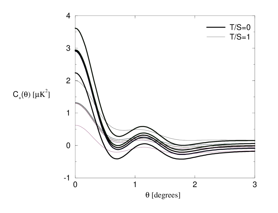
FIG. 3.: Full-sky averaged correlation function $C_{+}(\theta)\pm\Delta C_{+}(\theta)$. In each model, the correlation function is denoted by a middle line sandwiched by two pairs of $1\sigma$ lines. The outer pair of lines is for the MAP configuration, while the inner pair for the Planck Surveyor.

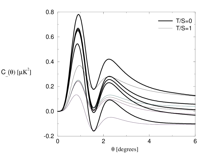
FIG. 4.: Full-sky averaged correlation function $C_{-}(\theta)\pm\Delta C_{-}(\theta)$ for MAP and Planck.

FIG. 5.: Full-sky averaged correlation function $C_{C}(\theta)\pm\Delta C_{C}(\theta)$ for MAP and Planck.

FIG. 6.: Full-sky averaged correlation function and its variance, $C_{T}(\theta)\pm\Delta C_{T}(\theta)$, for SPOrt/ISS experiment. In each model, the correlation function is denoted by a middle line sandwiched by a pair of $1\sigma$ lines. Solid and dashed lines denote respectively the models with reionization redshifts $z_{\rm ri}=50$ and $20$.

FIG. 7.: Full-sky averaged correlation function $C_{+}(\theta)\pm\Delta C_{+}(\theta)$ for SPOrt/ISS.

FIG. 8.: Full-sky averaged correlation function $C_{-}(\theta)\pm\Delta C_{-}(\theta)$ for SPOrt/ISS.

FIG. 9.: Full-sky averaged correlation function $C_{C}(\theta)\pm\Delta C_{C}(\theta)$ for SPOrt/ISS.