Spectral Observations of Diffuse FUV Emission from the Hot Phase of the Interstellar Medium with DUVE (the Diffuse Ultraviolet Experiment)

Abstract

One of the keys to interpreting the character and evolution of interstellar matter in the galaxy is understanding the distribution of the low density hot ($10^{5}{\rm\ K\,}-10^{6}{\rm\ K\,}$) phase of the interstellar medium (ISM). This phase is much more difficult to observe than the cooler high density components of the ISM because of its low density and lack of easily observable tracers. Because gas of this temperature emits mainly in the far ultraviolet (912 $\rm\AA$ - 1800 $\rm\AA$ ) and extreme ultraviolet (80 $\rm\AA$ - 912 $\rm\AA$ ), and (for gas hotter than $10^{6}$ K) X-rays, observations in these bands can provide important constraints to the distribution of this gas. Because of interstellar opacity at EUV wavelengths, only FUV and X-ray observations can provide clues to the properties of hot gas from distant regions. We present results from a search for FUV emission from the diffuse ISM conducted with an orbital FUV spectrometer, DUVE, which was launched in July, 1992. The DUVE spectrometer, which covers the band from 950 $\rm\AA$ to 1080 $\rm\AA$ with 3.2 $\rm\AA$ resolution, observed a region of low neutral hydrogen column density near the south galactic pole for a total effective integration time of 1583 seconds. The only emission line detected was a geocoronal hydrogen line at 1025 $\rm\AA$ . We are able to place upper limits to several expected emission features that provide constraints on interstellar plasma parameters. We are also able to place limits on the continuum emission throughout the bandpass. We compare these limits and other diffuse observations with several models of the structure of the interstellar medium and discuss the ramifications.

1 Introduction

Since the prediction of the existence of hot gas in the interstellar medium (ISM) by Spitzer (1956) and its subsequent detection by Bowyer, Field and Mack (1968) in Soft X-ray emission, a variety of models have been developed which attempt to explain the source of this gas, and how it evolves over time. The three dominant types of model, Galactic fountain models (Shapiro & Field (1976)), three phase models (McKee & Ostriker (1977)), and isolated supernova type models (Smith & Cox (1974)), all claim some measure of success in fitting the existing observations.

In the past several decades, measurements of interstellar absorption in the far ultraviolet (FUV) spectra of many stars using Copernicus and IUE (Jenkins 1978a&b, Savage & Massa 1987) have resulted in the detection of many highly ionized species. More recently the Goddard High Resolution Spectrometer (GHRS) on the Hubble Space Telescope, and the Berkeley FUV/EUV Spectrometer on ORFEUS (Sembach et al.  (1995); Spitzer (1996); Hurwitz & Bowyer (1996)) have provided additional data in this area.

Absorption measurements are fairly insensitive to the distribution of absorbing material along the line of sight and do not provide enough information to distinguish between various models of the ISM. Emission from the ISM, though difficult to detect, has been the subject of various investigations. Martin and Bowyer (1990) investigated emission in the FUV between 1300 and 1800 $\rm\AA$ using the Space Shuttle-borne UVX experiment. They detected Civ $\lambda\lambda$ 1548,1551 and Oiii] $\lambda\lambda$ 1661,1666 emission along several lines of sight.

Several attempts have been made to measure diffuse line emission between 900 and 1200 $\rm\AA$ . Voyager observations made by Holberg produced an upper limit of about $10^{4}$ $\rm ph\ s^{-1}$ $\rm cm^{-2}\ str^{-1}$ for Ovi $\lambda\lambda$ 1032,1038 (Holberg (1986)). However, these Voyager observations have recently been called into question by Edelstein, Bowyer and Lampton (1997). A similar limit for the Ovi doublet of $1.4{\times 10^{4}}{\rm\ ph\ s^{-1}\,}{\rm\ cm^{-2}\ str^{-1}\,}$ was also reached by Edelstein and Bowyer (1993). More recently Dixon et al. (1996) used the Hopkins Ultraviolet Telescope (HUT) to search for diffuse FUV emission. They observed ten lines of sight at high galactic latitude and claim detections of Ovi emission along four of the ten lines of sight. Dixon et al. determined that the Ovi  they measured was consistent with temperatures and pressures which are as much as an order of magnitude higher than those determined by Martin and Bowyer’s Civ measurements. Therefore they concluded that the Ovi they saw was produced by gas that is distinct from that which produces Civ emission.

2 The Instrument and Calibration

We have designed an instrument capable of measuring the important Ovi $\lambda\lambda$ 1032,1038 emission from the diffuse interstellar medium. The instrument’s small bandpass (150 $\rm\AA$ ) around the Ovi lines also includes the potentially important Ciii $\lambda$ 977, Niii $\lambda$ 991, and Cii $\lambda$ 1037 lines. Many problems need to be solved in the design of a diffuse spectrometer for this bandpass. The low predicted intensity of these emission lines requires that the spectrometer have a high effective area $\times$ solid angle product. In addition, sources of instrument background and spectral contamination must be limited. We discuss, in turn, important sources of background and the techniques used to mitigate them.

There are several bright airglow lines which could interfere with attempts to observe the faint Ovi $\lambda\lambda$ 1032,1038 lines. Predictions of Ovi emission indicate the intensity of these line should be near 5000 $\rm ph\ s^{-1}$ $\rm cm^{-2}\ str^{-1}$ (Shull & Slavin (1994)). The airglow lines nearest to the Ovi doublet, Hi $\lambda$ 1025 and Oi $\lambda$ 1027, have a combined intensity of about $10^{5.5}$ $\rm ph\ s^{-1}$ $\rm cm^{-2}\ str^{-1}$ . Assuming Gaussian line profiles, it can be shown that a spectral resolution of 2.7 $\rm\AA$ half-energy width (HEW) is required if the contribution to a bin at 1032 $\rm\AA$ is to contain less than 5000 $\rm ph\ s^{-1}$ $\rm cm^{-2}\ str^{-1}$ equivalent background due to these lines. For this reason, high spectral resolution is required to prevent contamination of the faint interstellar emission lines.

An even more troubling background source is the far brighter Hi $\lambda$ 1216 line. With an intensity of 5 kiloRaleighs (4 $\times 10^{8}$ $\rm ph\ s^{-1}$ $\rm cm^{-2}\ str^{-1}$ ), scattering within the instrument could easily swamp any signals. Hi $\lambda$ 1216 photons have to be rejected to a level of 5 $\times 10^{-6}$ per spectral bin or less to have an equivalent contribution of 5000 $\rm ph\ s^{-1}$ $\rm cm^{-2}\ str^{-1}$ . Unfortunately no filter material exists which is able to block Hi $\lambda$ 1216 while allowing Ovi $\lambda\lambda$ 1032,1038 to pass. A double spectrometer method was used to limit Hi $\lambda$ 1216 scattering as described below.

Another potential contaminant in the diffuse FUV spectrum is stellar flux. Bright O, B, and A stars can be eliminated simply by not pointing the instrument near any known bright stars of this type. Emission from later FUV emitting stars is more difficult to deal with. We designed our instrument with imaging along the slit to allow identification of stellar signals. We also used an additional detector which provided an FUV image of the spectrometer field. This allowed detection of stars too faint to be seen directly in the spectra.

A background due to exospheric charged particles is potentially quite substantial. This background can range from 1 $\rm s^{-1}cm^{-2}$ to upwards of $10^{5}$ $\rm s^{-1}cm^{-2}$ for an open faced microchannel plate detector. It is highly dependent on orbital parameters, especially ram angle, solar angle, altitude and position over the earth’s surface. In our instrument, the entrance aperture is covered with a fine mesh charged to +28 Volts to limit the number of exospheric charged particles that can reach the detector. In addition, an opaque shutter was employed to provide an in-flight determination of the entire non-photonic background.

The instrument, designated DUVE, the Diffuse Ultraviolet Experiment, is based on a spectrometer previously developed by Edelstein and Bowyer (1993). However, the DUVE instrument’s capability for studying diffuse radiation was substantially improved. The basic design is a two stage spectrometer which solves many of the background problems described above, yet provides a large area $\times$ solid angle product when compared to alternative designs. A schematic of the instrument is shown in Figure 1.

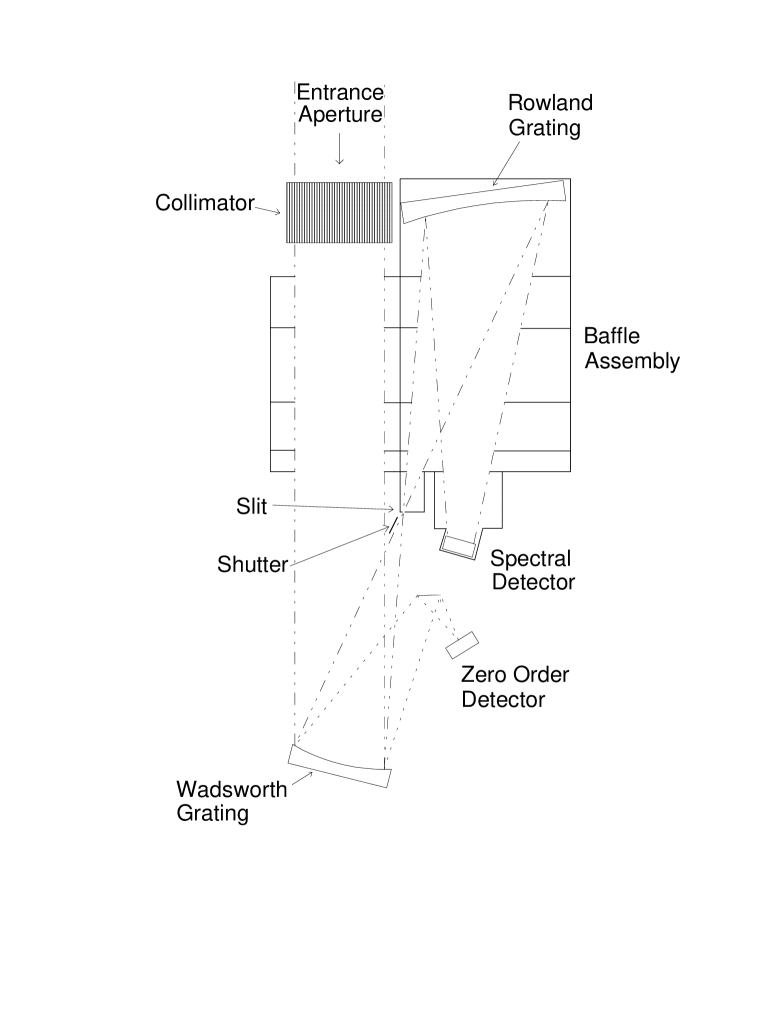
Figure 1: A schematic of the DUVE instrument. The dot-dash lines represent the light path from entrance aperture to spectral detector. The dotted line represents the path of zero order light from the Wadsworth grating.

The first stage of the spectrometer filters out unwanted wavelengths, most notably Hi $\lambda$ 1216. Light entering the spectrometer passes through a wire grid collimator with a full width of $\pm 1{{}^{\circ}}$. After passing through the collimator, the light strikes a diffraction grating in Wadsworth configuration. First order light from the grating is focused toward a slit. The slit width defines the horizontal (across the slit) sky acceptance angle. Contrary to intuition, this slit does not limit the instrument bandwidth. The collimator’s angular width and the Wadsworth grating ruling density define the width of the instrument bandpass. Each individual wavelength accepted by the slit has entered the collimator at a slightly different angle. This has the unique advantage of limiting contamination by a bright star to a wavelength range much smaller than the overall bandpass.

The second stage of the spectrometer is a dispersion stage. Light entering through the slit strikes a holographically corrected diffraction grating in a Rowland circle configuration. The second order diffracted light from the grating is focused onto a microchannel plate detector. Use of second order light in the diffraction stage allows high dispersion without significantly increasing the line density required to achieve the required spectral resolution. The spectral resolution of the second stage is determined by properties of the diffraction grating and the width of the entrance slit. Unwanted orders are blocked in this stage of the spectrometer through use of strategically placed baffles. They are specifically designed to eliminate all orders of Hi $\lambda$ 1216 which may have been scattered through the entrance slit.

Extensive calibration of the DUVE instrument was carried out using the EUV/FUV calibration facilities at the Space Sciences Laboratory (Welsh et al.  (1989)). The details of this calibration are beyond the scope of this paper, but are described in detail by Korpela (1997). In brief, all the components needed to calculate the effective (efficiency$\times$area$\times$solid angle) product (the instrument grasp) were measured at a variety of wavelengths. The result is shown in Figure 2.

Figure 2: DUVE area solid-angle product or grasp

The spectral resolution was also measured. The instrument was found to have a HEW of 3.5 $\rm\AA$ at 1025 $\rm\AA$ . However, the line profile was found to be asymmetric with a much steeper cutoff toward long wavelengths. Consequently the contribution of Hi $\lambda$ 1025 into a spectral bin at 1032 $\rm\AA$ is the same as an equivalent symmetric line with an HEW of 2.3 $\rm\AA$ . The imaging focus along the slit was also measured and was found to be $\sim 4$ arc minutes HEW.

3 The Flight

The DUVE instrument was launched as a secondary payload attached to the second stage of a Delta II 7925 vehicle on 24 July, 1992. As a secondary payload, the parameters of the DUVE orbit were determined by the requirements of the primary payload, the Geotail satellite. The orbital apogee was 1460 km which placed the instrument well above the majority of atomic oxygen airglow and above about half of the expected geocoronal hydrogen airglow.

Due to safety requirements, the propellant and control gases of the second stage had to be depleted by the end of the first orbit. Therefore the mission was conducted in two phases, a pointed phase for the first orbit, and a spin stabilized phase thereafter. Because the DUVE data were telemetered through the second stage telemetry system, the mission lifetime for DUVE was limited by the battery power available to the telemetry system (about 8 hours total).

During the first orbital night, the instrument was pointed at the primary target and a slow drift (0.1 ^∘ min^-1 perpendicular to the slit) was initiated. This phase continued until T+5000 seconds, at which time second stage spin up was begun. Observations continued throughout this period, however, much of the data were contaminated by stars and bright airglow. The primary target was an area of low neutral hydrogen column density and enhanced soft X-ray emission near $l=10^{\circ}$, $b=-60^{\circ}$. Because of the spin and its precession throughout the orbit, $\sim 2.3$ steradians of sky was sampled during the observations.

In flight, overall background rates ranged from 1 $\rm s^{-1}cm^{-2}$ to 20 $\rm s^{-1}cm^{-2}$ with a median value of 2 $\rm s^{-1}cm^{-2}$ , indicating that the methods employed to reduce the background in the instrument were quite successful. Overall, our backgrounds consisted of roughly equal parts charged particle background and intrinsic detector background. No scattered Hi $\lambda$ 1216 was detected.

4 Observational Results

Detector images (256 pixels spectral $\times$ 32 pixels imaging) were telemetered from the spacecraft during ground station contacts. These images were telemetered multiple times over many ground station passes, hence, many data dropouts were able to be corrected. The end result was 19 images obtained from 4151 seconds of observation time. These images were examined for stellar contamination, uncorrected data dropouts and instrument anomalies and the affected portions were masked off or otherwise corrected. Where no correction was possible, the images were discarded.

The sky and shuttered background images are accumulated in an interleaved fashion, each sky image has a corresponding background image. The telemetered images were ordered in terms of count rate in the background image. We then determined whether adding the next higher background image to the summed low noise set would decrease the overall noise rate ($\sqrt{\frac{N_{\rm bg}}{t}}$). Fifteen of the images passed this test. The background level of those images ranged from 1.0 to 2.6 cm^-2 s^-1. The background levels of those rejected ranged from 8.2 to 20 cm^-2 s^-1.

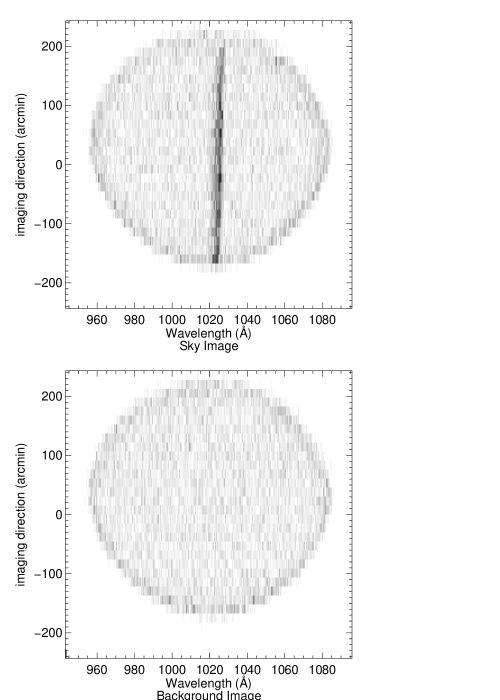
Figure 3: Raw spectral detector images from the DUVE instrument’s flight. The top image is a sum of shutter open images. The vertical stripe is Hi $\lambda$ 1025 airglow. The bottom image is a sum of the corresponding shutter closed images. Integration times are 1583 and 1529 seconds respectively.

The resulting sum of the accepted images is shown in Figure 3. The top image is a sum of shutter opened images. The vertical stripe is Hi $\lambda$ 1025 airglow. The bottom is a sum of the corresponding shutter closed images. The image has not been corrected for distortions.

Figure 4: The solid line represents the flight spectral data after subtraction of the background image and convolution with a line spread function. The dashed lines represent $\pm 3\sigma$ error levels.

The summed image was corrected for image distortions and shutter open/closed time, and the background image was subtracted from the data. The resulting image was histogrammed and convolved with a line spread function that was determined during calibration. The convolved histogram is shown in Figure 4. The dashed lines represent $\pm 3\sigma$ error levels as determined through count statistics and the error in the determination of the shutter open/closed time. This quantity is determined by:

$$\sigma = \sqrt{\sigma_{\rm fg}^{2}+\sigma_{\rm bg}^{2}+\sigma^{2}_{\Delta t}}$$ (1)

$$= {\sqrt{\left(\frac{N_{\rm fg}}{t_{\rm fg}}\right)^{2}+\left(\frac{N_{\rm bg}}{t_{\rm bg}}\right)^{2}+\left(\frac{N_{\rm fg}\Delta t}{t_{\rm fg}^{2}}+\frac{N_{\rm bg}\Delta t}{t_{\rm bg}^{2}}\right)^{2}}}$$

The quantities $N_{\rm fg}$ and $N_{\rm bg}$ are the number of counts (post-convolution) per wavelength bin in the sky and background images respectively. The values $t_{\rm fg}$ and $t_{\rm bg}$ represent the shutter open and shutter closed integration times (1582.6 and 1529.2 s) and $\Delta t$ represents the uncertainty in those times (14.0 s). The hatched area near the baseline in Figure 4 represents the approximate fraction of the error that is due to potential errors in shutter timing.

It can easily be seen that only one spectral line exceeds the $3\sigma$ significance level. That line is the geocoronal Hi $\lambda$ 1025 line. By dividing the count rate in this line by the DUVE grasp, we determined its intensity. The 1.31 counts per second detected corresponds to an intensity of $2.26\pm 0.26{\times 10^{5}}{\rm\ ph\ s^{-1}\,}{\rm\ cm^{-2}\ str^{-1}\,}.$ As expected this value is between that measured at low altitude (600 km) (Chakrabarti et al.  (1984)) and the interplanetary value (Holberg (1986)).

Figure 5: Upper limits to line emission placed by this work are shown as a solid line. Previous limits by Edelstein and Bowyer (1993) are shown by a dashed line. Limits determined from Voyager UVS measurements as analyzed by Edelstein, Bowyer, and Lampton (1997) are presented as a dot-dash line. The diamond with error bars is a measurement of OVI 1032,1038 $\rm\AA$ emission by Dixon et al. (1996). The vertical lines show the positions of several important astrophysical lines.

Species	${\lambda}({\rm\ \AA\,})$	$I({\rm\ ph\ s^{-1}\,}{\rm\ cm^{-2}\ str^{-1}\,})$	$I({\rm\ erg\ s^{-1}\ cm^{-2}\ str^{-1}\,})$
Hi	972	$\leq$ 7.4$\times 10^{4}$	$\leq$ 1.5$\times 10^{-6}$
Ciii	977	$\leq$ 4.0$\times 10^{4}$	$\leq$ 8.1$\times 10^{-7}$
Oi 1	989	$\leq$ 6.1$\times 10^{3}$	$\leq$ 1.2$\times 10^{-7}$
Niii	991	$\leq$ 5.5$\times 10^{3}$	$\leq$ 1.1$\times 10^{-7}$
Siii	992	$\leq$ 5.7$\times 10^{3}$	$\leq$ 1.1$\times 10^{-7}$
Siiii	996	$\leq$ 1.6$\times 10^{4}$	$\leq$ 3.2$\times 10^{-7}$
Nevi	1006	$\leq$ 1.3$\times 10^{4}$	$\leq$ 2.6$\times 10^{-7}$
Arvi	1008	$\leq$ 1.0$\times 10^{4}$	$\leq$ 2.0$\times 10^{-7}$
Hi 1,	1025	2.26$\pm$0.26$\times 10^{5}$	4.38$\pm$0.49 $\times 10^{-6}$
Ovi	1032, 1038	$\leq$ 7.6$\times 10^{3}$	$\leq$ 1 .4$\times 10^{-7}$
Cii	1037	$\leq$ 3.9$\times 10^{3}$	$\leq$ 7.4$\times 10^{-8}$
Ari 1	1050	$\leq$ 6.4$\times 10^{3}$	$\leq$ 1.2$\times 10^{-7}$
Siiv	1067	$\leq$ 2.9$\times 10^{4}$	$\leq$ 5.4$\times 10^{-7}$
Siv	1070	$\leq$ 5.1$\times 10^{4}$	$\leq$ 9.5$\times 10^{-7}$

Table 1: Upper limits to line emission placed by the DUVE data

We have used the DUVE data to derive upper limits to line emission in the band covered by the spectrometer. These limits are shown in Table 1. As a test of the error levels, fluctuations in the spectrum outside of the 1025 $\rm\AA$ line were compared with those expected by statistics. A histogram of the standard deviation per wavelength bin, $\frac{\Delta N}{\sigma}$, when compared to the zero level was best fit by a Gaussian of width $1.01\pm 0.03$ centered at $0.1\pm 0.1$.

Because the error in zero level is correlated over all wavelength bins, it represents the dominant source of uncertainty in the determination of the continuum limits. The contribution of this error is linear in the number of bins included, whereas the errors due to count statistics tend toward the square root of the number of bins. The best determinations of continuum level were $-1.07\pm 0.69\times 10^{3}{\rm\ ph\ s^{-1}\,}\-{\rm\ cm^{-2}\,}\-{\rm\ str^{-1}\-{\rm\ \AA\,}^{-1}\,}$ between 977 and 1020 $\rm\AA$ and $-3.2\pm 3.8\times 10^{2}{\rm\ ph\ s^{-1}\,}\-{\rm\ cm^{-2}\,}\-{\rm\ str^{-1}\-{\rm\ \AA\,}^{-1}\,}$ between 1028 and 1057 $\rm\AA$ . These measurements place 2$\sigma$ upper limits to the continuum in these spectral ranges of 310 and 440 $\rm ph\ s^{-1}$ $\rm cm^{-2}$ $\rm str^{-1}\-{\rm\ \AA\,}^{-1}$ respectively.

5 Comparison of results with models of the FUV background

5.1 Isothermal models

The simplest (and most often used) model of emission from the warm and hot phases of the interstellar medium is that of an optically thin, isothermal, collisionally excited plasma. This simple model does not take into account how the plasma was heated, nor any temperature variations within the plasma as it cools. For an emission line from a specific transition $(k\rightarrow j)$ from an ion $i$ the emitted intensity $I_{kj}$ is:

$$I_{kj}=\int_{0}^{\infty}\int_{0}^{\infty}j_{\nu}d\nu dx=h\nu_{kj}\int_{0}^{\infty}n_{i}n_{e}\gamma_{kj}dx$$ (2)

where $n_{i}$ is the density of the ion $i$ in the plasma and $n_{e}$ is the electron density. The quantity $\gamma_{jk}$ represents the collision strength into level $k$ and the probability of decay into level $j$. Determining this quantity is a complicated quantum mechanical calculation and is the subject of numerous papers. For the purposes of this discussion values from Landini and Monsignori-Fossi (1990) have been used. For an isothermal plasma equation 2 can be further reduced to:

$$I_{kj}=h\nu_{kj}{{n_{i}}\over{n_{\rm HI}}}{{n_{\rm HI}}\over{n_{e}}}\gamma_{jk}\int_{0}^{\infty}n_{e}^{2}dx$$ (3)

The quantities $\frac{n_{i}}{n_{\rm HI}}$ and $\frac{n_{\rm HI}}{n_{e}}$ can be determined from thermodynamics by assuming a temperature, density, and elemental abundances for the plasma. We use the abundances of Anders and Grevesse (1989). If the intensity $I_{kj}$ is measured and a temperature is assumed, only the value of the integral (known as the emission measure) is left as a free parameter. In practice, ratios of two emission lines, preferably from the same ion, are used to fix the temperature. If the temperature cannot be determined from observations, the emission measure is usually given as the locus of points over a range of temperatures that could produce the observed emission.

Using the upper limits obtained by the DUVE instrument, we can place upper limits to the emission measure of isothermal plasma models for the interstellar medium. In the case of local emission, such as would be expected to be associated with the gas in the local bubble, we would expect minimal dust absorption between us and the emitting gas. In this case, we can use the DUVE emission limits directly to obtain upper limits to the local emission measure.

Figure 6: Upper limit local emission measures derived from this work are shown as a solid line. The dashed lines represent X-ray emission measure limits derived for Wisconsin B and C band rocket borne observations in this direction (McCammon et al. 1983). The dot-dashed line represents emission measure limits determined from UVX (1400 to 1800 $\rm\AA$ ) observations by Martin and Bowyer (1990). The dotted line represents upper limits determined from EUVE observations by Jelinsky et al (1995). The hatched area is the parameter space cited by Paresce and Stern (1981) as being the allowed region to create observed broadband EUV and Soft X-ray emission with a single temperature plasma.

The emission measure of the interstellar medium is constrained by upper limits to five emission lines in this band. Although our observations were limited to $\sim 7500$ square degrees of sky, we assume that the results are global in nature. Although this is certainly not the case in detail, it is the only option we have given the limited number of ISM emission measurements. With this assumption we compare our results to the Martin and Bowyer results for Civ which sampled much smaller sky areas in several different directions. It should be noted that Martin and Bowyer detected Civ emission along every high galactic latitude line of sight they observed.

The lines that limit the emission measure are:

1. Mgii $\lambda$ 1027, which peaks at about $1.5{\times 10^{4}}$ K, constrains the emission measure at temperatures below $2.0{\times 10^{4}}$ K. Because of the nearby interference from Hi $\lambda$ 1025 emission, the observational limit obtained is high.

2. Cii $\lambda$ 1037, which peaks at a temperature of about 5$\times 10^{4}$ K, provides the best constraint for temperatures between $2.0{\times 10^{4}}$ and $5.1{\times 10^{4}}$ K. Because our simple model does not include photoionization, this may understate the constraint, as Cii is expected to be produced by photoionization due to FUV radiation from stars.

3. Ciii $\lambda$ 977, which peaks at $8.4{\times 10^{4}}$ K, provides the best constraint between $5.1{\times 10^{4}}$ and $1.0{\times 10^{5}}$ K.

4. Niii $\lambda$ 991, which peaks at 1$\times 10^{5}$ K, constrains the emission measure between 1.0$\times 10^{5}$ and 1.8$\times 10^{5}$ K.

5. Ovi $\lambda\lambda$ 1032,1038, which peaks at 2.8$\times 10^{5}$ K, provides upper limits to the emission measure above 1.8$\times 10^{5}$ K.

Figure 6 shows these emission measure upper limits. In this figure, the solid line represents limits to local emission measure derived from this work. The dashed lines represent emission measure limits determined by rocket borne broad band X-ray observations in the same direction as the DUVE observations (McCammon et al.  (1983)). The dot-dashed line represents limits to emission measure determined by Civ $\lambda\lambda$ 1548,1556 observations by Martin and Bowyer (1990). The dotted line represents upper limits determined by Jelinsky et al. (1995) from EUVE observations. The hatched area is the parameter space cited by Paresce and Stern (1981) as being the region allowed if broadband EUV and soft X-ray emission are produced by a single temperature plasma.

Figure 7: Upper limits to the emission measure of the galactic halo as derived by this work are shown as a solid line. The dot-dashed line represents limits to the halo emission as determined by Martin and Bowyer (1990) from UVX observations. The dashed lines represent B and C band observations by McCammon et al (1983). The dotted line represents emission measure limits of the warm ionized ISM as determined from optical observations by Reynolds (1991).

In the case where the emission is due to non-local gas, such as emission due to a hot galactic halo, we must consider absorption by intervening dust. Using the FUV extinction curve published by Sasseen et al (1996) and a standard gas to dust ratio, we are able to estimate the optical depth of dust per unit hydrogen column, or equivalent cross section. This equivalent cross section varies nearly linearly between 3.4$\times 10^{-21}$ cm² at 950 $\rm\AA$ to 2.6$\times 10^{-21}$ cm² at 1080 $\rm\AA$ . Along the lines of sight of the DUVE observations, the mean galactic Hi column density is 4.5$\times 10^{20}$ cm^-2 resulting in optical depths of between 1.2 and 1.5 and extinctions (1-$e^{-\tau}$) of 72% at 1032 $\rm\AA$ . This raises the emission measure limits by a factor of ${e^{\tau}}$, which is between 3.3 and 4.1 over our wavelength range. These upper limits to halo emission measure are shown in Figure 7. As with the previous figure, the dashed lines represent the Wisconsin soft X-ray observations and the dot dashed lines represent the Martin and Bowyer FUV observations. Both these measurements were corrected for dust absorption associated with a hydrogen column of 4.5$\times 10^{20}$ $\rm cm^{-2}$ . The dotted line is the emission measure determined from optical observations by Reynolds (1991) for the warm ionized phase of the ISM.

The points where the lines representing various determinations of these limits cross can be used to provide limits to the temperature of the isothermal models. The results in Figures 6 and 7 show that the DUVE observations limit the temperature of an isothermal model of the emission observed by Martin and Bowyer to between 5$\times 10^{4}$ and 2.2$\times 10^{5}$ K. The temperature of an isothermal model of the gas observed in the soft X-rays must be at a temperature above 5$\times 10^{5}$ K.

5.2 Evolutionary Models

Following Edgar and Chevalier (1986), we examine line emission from the hot interstellar medium in a simple evolutionary model by considering a constant source of gas at $T_{\rm hot}$ and a sink of gas at $T_{\rm cold}$; we assume that the mass flow rates at each temperature are equal and constant. The emergent intensity of a specific line in such a model is:

$$I_{kj}=h\nu_{kj}\int_{T_{\rm cold}}^{T_{\rm hot}}\frac{n_{\rm OVI}}{n_{\rm HI}}\frac{n_{\rm HI}}{n_{e}}\gamma_{kj}(T){{d(EM)}\over{dT}}dT$$ (4)

where EM has its usual definition. This can be simplified by making assumptions about the pressure/density evolution (isobaric or isochoric) and the ionization state of the material involved. Even without such assumptions, the intensity can be calculated numerically by assuming a pressure, density, and temperature distribution.

Because of the importance of nonequilibrium ionization effects in low density collisionally ionized gas at the temperature range in question, the assumption of ionization equilibrium may not hold in many cases. Solving for the nonequilibrium ionization state in the absence of photoionization requires solving a system of linear differential equations of the form

$$\frac{dX_{i}}{dt}=n_{e}\left[C^{ion}_{i-1}X_{i-1}-(C^{ion}_{i}+C^{rec}_{i})X_{i}+C^{rec}_{i+1}X_{i+1}\right]$$ (5)

where $X_{i}$ represents the fractional abundance of element $X$ in ionization state $i$. The $C^{ion}_{i}$ terms represent all collisional processes leading to ionization from state $i$ to state $i+1$. The $C^{rec}_{i}$ terms represent all processes leading to recombination from state $i+1$ to state $i$. These rate coefficients can further be subdivided into

$$C^{ion}_{i}=C_{elec}^{ion}(i,T)+C^{ion}_{auto}(i,T)+C^{ion}_{c-t}(i,T)$$ (6)

$$C^{rec}_{i}=C_{rad}^{rec}(i,T)+C^{rec}_{2-e}(i,T)+C^{rec}_{c-t}(i,T).$$ (7)

The rate coefficient for ionization by collisions with electrons is $C^{ion}_{elec}$, $C^{ion}_{auto}$ is the rate coefficient for excitation autoionization, $C_{rad}^{rec}$ is the rate coefficient for radiative recombination, and $C_{2-e}^{rec}$ is the rate coefficient for dielectronic recombination. The $C^{ion}_{c-t}$ and $C^{rec}_{c-t}$ terms represent rates for charge transfer ionization and recombination. Because these rates are in general important only for charge transfers from hydrogen and helium atoms to more highly ionized atoms, and because hydrogen and helium are fully ionized in the temperature range of interest, we will ignore these terms. The approximations for these coefficients were taken from Arnaud and Rothenflug (1985), and Shull and Van Steenberg (1982).

By assuming a fully ionized plasma of 90% hydrogen and 10% helium as the source of the electron density ($n=1.91n_{e}$), we can solve the set of equations for each element individually. Because the set of equations is stiffly coupled and therefore subject to numerical instability, we integrated them using an implicit multistep stiffly stable method described by Gear (1971).

We determined a cooling rate from a radiative cooling curve $\Lambda(T)$ and assumed density structure $n(t)$.

$$\frac{dT}{dt}=-\frac{2\Lambda(T)}{3nk}+\frac{2T}{3n}\frac{dn}{dT}$$ (8)

$$\frac{dT}{dt}=\left\{\begin{array}[]{ll}-\frac{2\Lambda(T)}{3nk}&\mbox{\rm isochoric\ cooling}\\ -\frac{2\Lambda(T)}{5nk}&\mbox{\rm isobaric\ cooling}\end{array}\right.$$ (9)

Equations 7–9 thus become

$$\frac{dX_{i}}{dT}={{\frac{dX_{i}}{dt}}\over{\frac{dT}{dt}}}=\frac{Kn_{e}^{2}k}{\Lambda(T)}\left[C^{ion}_{i-1}X_{i-1}-(C^{ion}_{i}+C^{rec}_{i})X_{i}+C^{rec}_{i+1}X_{i+1}\right]$$ (10)

where $K$=2.87 for isochoric cooling and $K$=4.78 for isobaric cooling.

The initial conditions for the problem were considered to be the equilibrium ionization values at the starting temperature ($T_{\rm hot}=10^{7}$ K). The quantity $\Lambda(T)$ was calculated using the emission code of Landini and Monsignori Fossi (1990) using our calculated ionization fraction. New ionization fractions for important elements were calculated numerically using the integration code described above. The emission was then recalculated using the new ionization fractions and summed over all elements to obtain a new $\Lambda(T)$. The procedure was iterated until $\Lambda(T)$ converged.

In this model we assumed the dominant cooling mechanism was radiative cooling. Thus the time a parcel of material spends in a given temperature range, and therefore the total amount of material in that range, is inversely proportional to the rate of cooling of that material. Following standard practice we considered three density/pressure constraints: 1) isobaric evolution wherein all the gas is in pressure equilibrium, 2) isochoric evolution in which all the gas is at a constant density and 3) a mixed model in which the gas initially evolves isochorically and then at some temperature begins to evolve isobarically. Using the value of the intensity of Civ emission as determined by Martin and Bowyer, we can calculate the expected intensity at Ovi $\lambda\lambda$ 1032,1038. In the case of an isobaric model, an Ovi intensity of 1.9$\times 10^{4}$ $\rm ph\ s^{-1}$ $\rm cm^{-2}\ str^{-1}$ is predicted, which is a factor of 2.5 greater than our observed upper limit. In the case of an isochoric model, the predicted intensity is 5$\times 10^{3}$ , which is somewhat below the upper limit. Mixed models fall between these values depending on the temperature of the isochoric-isobaric transition. These models will be discussed further in Section 5.5.

5.3 The Smith and Cox model

Smith and Cox (1974) developed a model of the ISM based on an estimate of the volume of the interstellar medium occupied by supernova remnants. They considered the expansion of isolated supernova remnants with energy 4$\times 10^{50}$ erg in an ambient medium of density 1.0 cm^-3. This calculation resulted in remnants of radius $\sim 40$ pc which persist for 4$\times 10^{6}$ years. They calculated a “porosity” of the ISM, $q=r\tau V_{\rm SNR}$ where $r$ is the average supernova rate per unit volume, $\tau$ is the lifetime of an isolated SNR, and $V_{\rm SNR}$ is the time averaged volume of the SNR over this lifetime. Their calculation indicated that the value of $q$ was near 0.1. They also estimated that the probability of intersection of a SNR with other remnants was about 50%, and showed these interactions were an important key to the state of the ISM.

Slavin and Cox (1992, 1993) revised the Smith and Cox model to describe the spherically symmetric expansion of a supernova remnant into a warm medium of density 0.2 $\rm cm^{-3}$ and temperature $10^{4}$ K. Their model includes a magnetic field in the ambient medium which serves to apply an additional nonthermal pressure against the expansion. They assumed that compression and expansion of the matter in the remnant results in a magnetic field that is proportional to the mass density, which is valid for plane parallel shocks. Their model assumed a magnetic field in the ambient medium of 5 $\rm\mu G$ . Because this is a one dimensional model, we would expect these calculations to be valid only along the magnetic equator of a supernova remnant.

The result of their simulation was a bubble of hot gas which reaches its maximum radius of $\sim 55{\rm\ pc\,}$ after about 1$\times 10^{6}$ years. Following this, the bubble slowly collapses on a time scale of $\sim 5.5{\times 10^{6}}$ years. Surprisingly, during the collapse, the central temperature stays roughly constant at about 3$\times 10^{5}$ K, while the density inside the remnant increases.

In extending their model from an individual supernova to a model of the interstellar medium, they assumed supernovae distributed randomly throughout the disk with an exponential scale height of 300 $\rm pc$ . They determined the dependence of the maximum radius, expansion time, and collapse time with variations in the magnetic field, gas density, and supernova energy. They used these to determine a global average time integrated volume for a supernova, and used this value to determine the volume filling factor of supernova remnants. They found a porosity $q\leq 0.18$. Even with this higher limit for the filling factor, their model shows fewer interactions between remnants than would be expected from the earlier model of Smith and Cox. The mean free path between bubbles and Ovi  column density per bubble in this model closely matches that determined from the analysis of Copernicus observations by Shelton and Cox (1994).

For the purpose of comparing FUV emission measurements to a Slavin and Cox model it was necessary to simplify the model to some degree. Rather than duplicate their entire MHD calculation, we digitized several figures from their articles containing the density, temperature, velocity, and total pressure profiles of the remnant at various times. We were able to fit these curves with Chebyshev polynomials with time varying coefficients to produce an approximation of the profiles. Using these density, temperature, pressure, and velocity profiles we were able to calculate the non-equilibrium ionization and the corresponding line emission for a “standard” supernova remnant using the method described in Section 5.2. Our simplified model closely matches the results obtained by Slavin and Cox.

We next modeled the appearance of the sky. This required several assumptions. Slavin and Cox assumed a constant midplane supernova rate of 0.4$\times 10^{-13}$ $\rm pc$ ^-3 yr^-1, and a supernova scale height of 300 pc. For the purpose of modeling sky coverage, they assumed that all supernovae are “standard” supernovae of energy 5$\times 10^{50}$ ergs, occurring in a medium of density 0.2 $\rm cm^{-3}$ , temperature of 10000 K, and magnetic field of 5 $\rm\mu G$ . We modeled limb brightening effects in the remnant by assuming the ions were uniformly distributed within a spherical shell with inner and outer radii determined by the radii where $n_{i}n_{e}={\rm max}(n_{i}n_{e})/2$. Absorption by interstellar dust was modeled by assuming a constant gas/dust ratio. We considered an Hi distribution with three components: a Gaussian component of scale length 110 parsecs with central density 0.39 $\rm cm^{-3}$ , a Gaussian component of scale length 260 parsecs and central density 0.11 $\rm cm^{-3}$ , and an exponential component of scale height 400 parsecs and a central density of 0.06 $\rm cm^{-3}$ . The distribution of H₂ was modeled as an exponential distribution with a central density of 1.333 $\rm cm^{-3}$ and with scale height 55 $\rm pc$ (Dickey & Lockman (1990); Dame & Thaddeus (1995); Savage (1995)). Interstellar opacities at 1032 $\rm\AA$ and 1550 $\rm\AA$ were determined with reference to Sasseen et al. (1996) and correspond to cross sections of 2.9$\times 10^{-21}$ $\rm cm^{2}$ N${}_{\rm H}^{-1}$ and 1.5$\times 10^{-21}$ $\rm cm^{2}$ N${}_{\rm H}^{-1}$ respectively. The distance to the remnants and the associated hydrogen column were assumed to be constant across the face of each remnant. A small component due to the local bubble was modeled as emission from a SNR with central temperature 2$\times 10^{6}$ K, and with a temperature gradient as specified by R. Smith (1996).

Emission for both Ovi $\lambda\lambda$ 1032,1038 and Civ $\lambda\lambda$ 1548,1551 were calculated. At both wavelengths the sky is faint, with the median sky intensities being $<{\rm{\rm\ I(OVI)\,}}>$ = 120 $\rm ph\ s^{-1}$ $\rm cm^{-2}\ str^{-1}$ and $<{\rm{\rm\ I(CIV)\,}}>$ = 350 $\rm ph\ s^{-1}$ $\rm cm^{-2}\ str^{-1}$ . Based on these calculations we estimate that less than 10% of the sky emits at the level of Civ seen by Martin and Bowyer, 5000 $\rm ph\ s^{-1}$ $\rm cm^{-2}\ str^{-1}$ . In addition to the difference in overall intensity, there is a difference in the distribution of the emission. The Civ intensity measured by Martin and Bowyer is at least a factor of two brighter near the galactic poles than near the galactic plane, whereas in the Slavin and Cox model, the majority of the emission is seen near the galactic plane.

This result seems to be fairly invariant to the major parameters of the model. Introducing a variation evolution of the remnants with altitude above the galactic plane, $z$, could increase the fractional sky coverage of remnants at high latitude. However, the intensity of a remnant is lower due to the lower densities, resulting in a longer lasting remnant. We expect these variations to come near to canceling, with the average sky intensity staying roughly constant. This effect should be included in future models and is currently the subject of study. (Shelton (1996))

Spatially and temporally correlated supernovae could also have an effect. Slavin and Cox’s calculations show a rough $\int Adt\propto E$ dependence at constant pressure parameters, thus we would expect the time integrated sky coverage of a single multiple event remnant to be proportional to the number of supernovae that occurred in the remnant, $N$. On the other hand, the number of such remnants present in the sky would be proportional to $\frac{1}{N}$. Therefore we expect the sky coverage of remnants to be roughly constant. The remnant lifetime is dependent on the radiative properties of the remnant. A rough estimate of the remnant luminosity can be made by assuming the energy radiated is proportional to the total energy of the supernovae, $N\times E_{sn}$, radiated through $\int Adt$ surface area and time. Again the factors cancel leaving the time averaged intensity unchanged.

5.4 The McKee-Ostriker model

McKee and Ostriker (1977, hereafter MO) presented a detailed model of the interstellar medium. The model assumed heating of the hot medium by supernovae, and cooling of the hot medium by radiation and with thermal pressure equilibrium between the warm clouds and the hot medium. By assuming a lower pressure and density in the ambient medium than that assumed by Smith and Cox, and a higher energy per supernova, they calculated a porosity $q$ which could exceed unity, rendering simple calculations of porosity invalid due to interaction of remnants. Therefore, they simply assumed that the filling factor of the hot gas was large. Using this, they devised a 3 phase model of the ISM, consisting, on average of warm ($10^{4}$ K) clouds (some with cool ($10^{2}$ K) cores) existing in pressure equilibrium with a hot ($10^{5.7-6.0}$ K) medium at pressure $10^{3.2}$ $\rm cm^{-3}$ K, and with an intermediate temperature evaporative region between the hot and warm components.

In principle, a simple constraint which could be placed upon the MO model is that of the filling factor of the hot medium, $f_{\rm hot}$. The Ovi emission measure that would be expected to be present along the DUVE line of sight is:

$${\rm EM}=5.7{\times 10^{-4}}\left[\frac{P}{2500{\rm\ {\rm cm}^{-3}{\rm K}\,}}\right]^{2}\left[\frac{T_{\rm hot}}{5{\times 10^{5}}K}\right]^{-5.2}\left[\frac{f_{\rm hot}}{0.6}\right]\left[\frac{h}{1{\rm\ kpc\,}}\right]{\rm\ {\rm cm}^{-6}{\rm pc}\,}$$ (11)

Unfortunately, this emission is less than the DUVE lower limit even with filling factors of 1. This shows that detecting the hot medium itself is a difficult task at FUV wavelengths. This is because the bulk of FUV emission in a MO model is produced by the interfaces between the warm and hot media.

To more accurately calculate expected emission from interfaces in a MO model, we used an analytic solution for conductive cloud boundaries as described by Dalton and Balbus (1993). This model describes both saturated and unsaturated evaporation of spherical clouds. Saturated evaporation occurs when the temperature gradients become large compared to the mean free path of electrons in the gas. This results in a breakdown in the local heat transport; energy is transported many temperature scale heights. The result is that the diffusive approximation ($q=-\kappa\nabla T$) is no longer valid, resulting in much lower heat flux than would be obtained by using the gradient of the temperature. The form of the solutions for density, temperature, and velocity profiles when parameterized to a unitless radius $y=\frac{r}{R_{\rm cloud}}$ and temperature $\tau=\frac{T}{T_{\rm hot}}$ has only one free parameter, the saturation parameter $\sigma_{o}$, which can be approximated as the ratio of the electron mean free path in the hot gas and the cloud radius.

Because the MO model is at pressure equilibrium, the cloud radius is determined by the mean Hi column density of the cloud. The model also provides velocities of the evaporating gas, which allow calculation of non-ionization equilibrium effects. It is assumed that the temperature distribution in this model is determined only by the gas flow and heat conduction, with no radiative losses. Because the gas flows toward regions of rapidly decreasing density, the high stage ions can persist much longer and to much greater radii than would be expected from collisional ionization equilibrium calculations.

We calculated the emission from evaporative cloud boundaries for clouds of varying radii at the “preferred” MO values of the temperature (5$\times 10^{5}$ K) and filling factor (0.6) and a variety of pressures. The resulting emergent intensities from the conductive boundaries were well fit by a power law. Given a power law distribution of clouds with slope ($\alpha$) and summed column density, N_HI, we can calculate the intensity of emission along the line of sight of the DUVE experiment. Using the power law described by Dickey and Lockman (1990) ($\alpha=-4.3$) for clouds with column density between 1.5$\times 10^{18}$ and 1.2$\times 10^{19}$ , we calculate a total emission integrated along the line of sight of

$$I_{\rm OVI}=1600\left(\frac{P}{2500{\rm\ {\rm cm}^{-3}{\rm K}\,}}\right)^{2}\left(1-e^{\frac{-N_{18}}{350}}\right)$$ (12)

$$I_{\rm CIV}=5300\left(\frac{P}{2500{\rm\ {\rm cm}^{-3}{\rm K}\,}}\right)^{2}\left(1-e^{\frac{-N_{18}}{650}}\right)$$ (13)

where $N_{18}$ is the total line of sight hydrogen column in units of 10¹⁸ $\rm cm^{-2}$ . Along the DUVE line of sight, this would result in Ovi and Civ emission of 1200 and 2700 $\rm ph\ s^{-1}$ $\rm cm^{-2}\ str^{-1}$ respectively.

Because this model depends upon the distribution of cloud sizes, which in turn effects the number of cloud interfaces along the line of sight, it is fairly sensitive to the power of the cloud size distribution. An increase in the power law slope from -4.3 to -3.3, causes a reduction in the number of small clouds. This results in an intensity reduction of a factor of two. Non spherical clouds, especially those with correlated orientations, or the inclusion of magnetic fields could also change these results.

Figure 8: The solid lines show the limits to filling factor in an McKee-Ostriker model placed by the DUVE data as a function of temperature for 3 assumed pressures. Pressures shown are 2500, 4000, and 16000 $\rm{\rm cm}^{-3}{\rm K}$ .

We repeated this calculation for a wide range of temperatures and filling factors. By assuming a given pressure, we can determine the locus of values of filling factor and temperature that would produce emission at the DUVE Ovi upper limit or Civ emission at the level of the Martin and Bowyer measurement. Such curves are plotted for 3 different pressures ( 2500, 4000, 16000 $\rm{\rm cm}^{-3}{\rm K}$ ) in Figure 8. The area below these curves represent allowed values of the temperature and filling factor.

5.5 Galactic fountain models

Shapiro and Field (1976) first described a “galactic fountain” model of the hot interstellar medium. They argued that the long cooling time of hot, low-density gas ($t{\rm\ >\,}10^{6}$ yrs) would allow time for the hot gas to rise buoyantly above the galactic plane. This gas would eventually cool radiatively, condense into clouds, and fall back to the plane. They argued that this model could explain both the presence of hot gas and infalling high velocity clouds.

Basic galactic fountain models follow the thermal evolution of hot gas. Most of these basic models assume that the gas starts its cooling at a constant density and then, at some point, it transitions to evolution at constant pressure. If we assume that the Civ emission observed by Martin and Bowyer is emission from a galactic fountain, we can use these simple models to determine what the expected Ovi intensity would be. These estimates were produced using the non-equilibrium ionization code described in Section 5.2. We again calculated the time integrated emission for a cooling gas parcel for both isobaric and isochoric cooling. We repeated this calculation over a wide range of initial temperatures from 10⁵ to 10⁷ K. We also repeated the calculations for models including an isochoric$\rightarrow$isobaric transition for transition temperatures ranging from 10⁵ to 10⁷ K. The values of Civ and Ovi intensity were corrected for differential absorption by dust associated with a hydrogen column of 4.5$\times 10^{20}$ $\rm cm^{-2}$ .

Figure 9: Ovi emission vs base temperature for simple galactic fountain models. Both isobaric and isochoric models are shown. The plot assumes 5000 $\rm ph\ s^{-1}$ $\rm cm^{-2}\ str^{-1}$ of measured Civ emission and dust absorption associated with an Hi column of 4.5$\times 10^{20}$ $\rm cm^{-2}$ . The dotted line represents the DUVE upper limit to Ovi emission.

Figure 10: Ovi emission vs transition temperature for simple galactic fountain models. The lower plot assumes 5000 $\rm ph\ s^{-1}$ $\rm cm^{-2}\ str^{-1}$ of Civ emission and dust absorption associated with an Hi column of 4.5$\times 10^{20}$ $\rm cm^{-2}$ . The dotted line represents the DUVE upper limit to Ovi emission.

Figure 9 shows calculations of Ovi emission vs the base temperature for simple isochoric and isobaric galactic fountain models scaled to the Martin and Bowyer Civ emission value. We can place an upper limit input temperature of 3.5$\times 10^{5}$ K on fully isobaric fountains. Fully isochoric fountains would produce Ovi emission at levels below the DUVE detection threshold. In Figure 10, we show models containing an isochoric/isobaric transition. We can limit the transition temperatures to less than 2$\times 10^{5}$ K.

Many far more complex models of galactic fountains have been published including effects outside of the realm of the simple model described above. They include such things as non-equilibrium ionization, turbulent mixing of hot and cold gas, and photoionization by the emitted EUV and X-ray radiation. However, a prediction of the ratio of $\frac{\rm I(OVI)}{\rm I(CIV)}$ and the intensity of Ovi emission per solar mass of circulation within the fountain can be obtained for each of these models. These predictions assume that the lines of sight observed by DUVE and UVX can be extrapolated to give a global average intensity across the entire galactic disk. The large solid angle observed by DUVE, (18% of the sky), makes it likely that this method of averaging is applicable. While this method of averaging is less applicable to the Martin and Bowyer Civ measurements with their smaller sampling solid angle, the fact that Civ was detected along every high-latitude line of sight could indicate that their measurements are typical of high latitude Civ emission.

The model by Edgar and Chevalier (1986) includes non-equilibrium effects at temperatures below 10⁶ K, and transitions between isochoric and isobaric evolution. They predict an emission at Civ $\lambda\lambda$ 1549 of 560-890 $\rm ph\ s^{-1}$ $\rm cm^{-2}\ str^{-1}$ for a mass flow of 4 M_⊙ yr^-1 and Ovi $\lambda\lambda$ 1032,1038 emission of 1600-2400 $\rm ph\ s^{-1}$ $\rm cm^{-2}\ str^{-1}$ . We can limit the mass flow rate in their model to less than 4.75 M_⊙ yr^-1. Their model also predicts $\frac{\rm I(OVI)}{\rm I(CIV)}=7.2-10.8$, a much higher value than our observed limit of $\sim$1.5. Again these are averages over the galactic disk and could be much brighter in some directions.

Houck and Bregman (1990) attempt to fit the observed scale height and velocity distribution of neutral gas clouds in the galaxy with a galactic fountain model. Their model does not include non-equilibrium ionization effects, which they concluded would have little effect on their results. Their results were calculated along a one dimensional grid. Their best fit to the distribution of neutral cloud velocities was a model with a base temperature of 3$\times 10^{5}$ K, a base pressure of 300 $\rm{\rm cm}^{-3}{\rm K}$ , and a mass flow rate of 0.2 M_⊙ yr^-1. Although Houck and Bregman did not include explicit predictions of FUV emission, we were able to use data from their paper to produce conservative lower limits to the equilibrium Civ and Ovi intensities of this model. By digitizing figures from their paper, we were able to estimate $I_{\rm OVI}$ to be approximately 1200 $\rm ph\ s^{-1}$ $\rm cm^{-2}\ str^{-1}$ per solar mass of flow and $\frac{\rm I(OVI)}{\rm I(CIV)}=0.3$. Both of these values are consistent with the DUVE observations as well as those of Martin and Bowyer. However, because this model is designed to match infalling clouds, changes in our understanding of these could could greatly change the predicted intensity.

Shull and Slavin (1994) added the effects of turbulent mixing of hot and cold gas into galactic fountain models. In this model, they calculate the ratio for emission $\frac{\rm I(OVI)}{\rm I(CIV)}=1.2\pm 0.2$ for $\log T=5.3\pm 0.3$, resulting in a predicted Ovi emission of 5000 to 7000 $\rm ph\ s^{-1}$ $\rm cm^{-2}\ str^{-1}$ at mass flow rates between 15 and 25 M_⊙ yr^-1. These predictions are based upon a range of mixing velocities, abundances, and mean temperatures. These parameters were used to determine the interstellar pressure required to produce the observed Civ emission. The $\frac{\rm I(OVI)}{\rm I(CIV)}$ ratio determined through this method is consistent with the DUVE observations. We are able to limit mass flow in this model to 21 to 38 M_⊙ yr^-1.

Model	Edgar &	Houck &	Shull &
	Chevalier 1986	Bregman 1990	Slavin 1994
Tmax (K)	$10^{6}$	3$\times 10^{5}$	$10^{5.3\pm 0.3}$
$\frac{\rm I({\rm O{\sc vi\ }})}{\rm\dot{M}[\odot]}$	1600-2400	1200	200-350
$\frac{\rm I({\rm O{\sc vi\ }})}{\rm I({\rm C{\sc iv\,}})}$	7.2–10.8	0.3	1.0–1.4
${\rm\dot{M}_{max}(M_{\odot}yr^{-1})}$	$\rm<$ 3.2–4.75	$\rm<$ 6.3	$\rm<$ 21–38

Table 2: Constraints to galactic fountain models.

The predicted Ovi intensities and the limits to mass flow rates in each of these models is shown in Table 2.

6 Discussion

Although the DUVE data are able to place constraints to the models discussed above, it is important to note that the model parameters are sufficiently flexible, the DUVE data alone cannot rule them out. The patchy distribution of the emitting gas in the galactic fountain and Smith and Cox models makes it possible, if somewhat unlikely, that the distribution of gas along the Martin and Bowyer lines of sight bears no resemblance to that sampled by the DUVE observations. Observations of both Civ and Ovi emission along the same line of sight would be extremely useful. The predicted distribution of these emissions varies from highly pole brightened (galactic fountain) to fairly uniform (MO models) to plane brightened (Smith and Cox), thus an all sky spectral survey of diffuse FUV emission would greatly enhance our understanding of the ISM.

7 Conclusions

We designed and built an instrument for the study of emission from the diffuse ISM at wavelengths between 950 and 1080 $\rm\AA$ . This instrument was flown on July 24, 1992 attached to the second stage of a Delta II launch vehicle. It achieved orbit and operated as planned, providing 4151 seconds of observations during orbital night periods.

Observations made by the DUVE instrument did not detect emission from the hot phase of the interstellar medium. We were, however, able to place new upper limits to emission from Ovi $\lambda\lambda$ 1032,1038 , Cii $\lambda$ 1037 , Ciii $\lambda$ 977, and Niii $\lambda$ 971 which significantly constrain the parameters of the hot ISM. We have used these limits to determine constraints to the emission measure of both local and halo gas between $10^{4}$ and $10^{6}$ K.

We have modeled Ovi and Civ emission from scattered supernovae and compared the results to our observations. Our model predicts emission at levels below the previously measured Civ values and the Ovi limits reported here.

We have modeled Ovi and Civ emission from clouds in a standard McKee Ostriker model. The produced emission in this model is also below the DUVE Ovi upper limits and the previously measured Civ values. We have placed limits to the filling factor of the hot medium versus its temperature.

We are able to place limits to the base temperatures and isochoric transition temperatures in simple galactic fountain models. Our observations are inconsistent with the I[Ovi ]/I[Civ ] ratios predicted by simple galactic fountain models with base gas temperatures of above about $10^{5.6}$K. Our observations are consistent with galactic fountain models with lower temperatures. Our observations place limits to the mass flow rates of several galactic fountain models.

8 Acknowledgements

We would like to thank Michael Lampton for his assistance with many aspects of this project, Charlie Gunn at NASA/OLS for providing the opportunity for this mission, the staff of the Space Sciences Lab and the McDonnell Douglas Delta Program Office for their assistance. This work has been supported by NASA grant NGR-05-003-805.

References

- Anders & Grevesse (1989) Anders, E. & Grevesse, N. 1989, Geochim. Cosmochim., 53, 197.
- Arnaud et al. (1985) Arnaud, M., & Rothenflug, R. 1985, A&AS, 60, 425.
- Bowyer, Field & Mack (1968) Bowyer, C. S., Field, G. B., & Mack, J. E. 1968, Nature, 351, 32.
- Chakrabarti et al. (1984) Chakrabarti, S., Kimble, R. & Bowyer, S. 1984, JGR, 89, 5660.
- Dalton & Balbus (1993) Dalton, W. W., & Balbus, S. A. 1993, ApJ, 404, 625.
- Dame & Thaddeus (1995) Dame, T. M., & Thaddeus, P. 1995, ASP Conf. Series, 80, 15.
- Dickey & Lockman (1990) Dickey, J. M., & Lockman, F. J. 1990, ARA&A, 28, 215.
- Dixon et al. (1996) Dixon, W. V., Davidsen, A. F. & Ferguson, H. C. 1996, ApJ, 465, 288.
- EBL (1997) Edelstein, J., Bowyer, S., and Lampton, M. 1997, Submitted to ApJ.
- Edelstein & Bowyer (1993) Edelstein, J. & Bowyer, S. 1993, AdSpR, v13, n12, 307.
- Edgar & Chevalier (1986) Edgar, R. J., & Chevalier, R. A. 1986, ApJ, 310, L27.
- Gear (1971) Gear, C. W. 1971, Numerical Initial Value Problems in Ordinary Differential Equations, (Englewood Cliffs: Prentice Hall).
- Holberg (1986) Holberg, J. B. 1986, ApJ, 311, 969.
- Houck & Bregman (1990) Houck, J. C., & Bregman, J. 1990, ApJ, 352, 506.
- Hurwitz & Bowyer (1996) Hurwitz, M., & Bowyer S. 1996, ApJ, 465, 296.
- Jelinsky et al. (1995) Jelinsky, P., Vallerga, J. V. & Edelstein, J. 1995, ApJ, 442, 653.
- (17) Jenkins, E. B. 1978a, ApJ, 219, 845.
- (18) Jenkins, E. B. 1978b, ApJ, 220, 107.
- Korpela (1997) Korpela, E. J. 1997, Ph. D. Thesis, University of California.
- Landini & Monsignori Fossi (1990) Landini, M., & Monsignori Fossi, B. C. 1990, A&AS, 82, 229.
- Martin & Bowyer (1990) Martin, C. & Bowyer, S. 1990, ApJ, 350, 242.
- McCammon et al. (1983) McCammon, D., Burrows, D. N., Sanders, W. T., Kraushaar, W. L. 1983, ApJ, 269, 107.
- McKee & Ostriker (1977) McKee, C. F. & Ostriker, J. P. 1977, ApJ, 218, 148.
- Paresce & Stern (1981) Paresce, F. & Stern, R. 1981, ApJ, 247, 89.
- Raymond (1992) Raymond, J. C. 1992, ApJ, 384, 502.
- Reynolds (1991) Reynolds, R. J. 1991, ApJ, 372, L17.
- Rosen, Bregman & Norman (1993) Rosen, A., Bregman, J. N., & Norman, M. L. 1993, ApJ, 413, 137.
- Sasseen (1996) Sasseen, T. P., Hurwitz, M., Dixon, W. V., Bowyer, S. 1996, BAAS, 188, 07.02.
- Savage & de Boer (1981) Savage, B. D., & Massa, D. 1987, ApJ, 314, 380.
- Savage (1995) Savage, B. D. 1995, ASP Conf. Series, 80, 233.
- Sembach et al. (1995) Sembach, K. R., Savage, B. D., & Lu, L. 1995, ApJ, 439, 672.
- Shapiro & Field (1976) Shapiro, P. R. & Field, G. B. 1976, ApJ, 205, 762.
- Shapiro & Benjamin (1991) Shapiro, P. R. & Benjamin, R. A. 1991, PASP, 103, 923.
- Shelton (1996) Shelton, R. L. 1996, Ph. D. thesis, University of Wisconsin.
- Shelton & Cox (1994) Shelton, R. L., & Cox, D. P. 1994, ApJ, 434, 599.
- Shull & Van Steenberg (1982) Shull, J. M., & Van Steenberg, M. 1982, ApJS., 48, 95.
- Shull & Slavin (1994) Shull, J. M., & Slavin, J. D. 1994, ApJ, 427, 784.
- Slavin & Cox (1992) Slavin, J. & Cox, D. 1992, ApJ, 392, 131.
- Slavin & Cox (1993) Slavin, J. & Cox, D. 1993, ApJ, 417, 187.
- Smith & Cox (1974) Smith, B. W., & Cox , D. P. 1974, ApJ, 189, L105.
- Smith (1996) Smith, R. K. 1996, Ph. D. Thesis, University of Wisconsin.
- Spitzer (1956) Spitzer, L. 1956, ApJ, 124, 20.
- Spitzer (1996) Spitzer, L. 1996, ApJ, 458, 29.
- Welsh et al. (1989) Welsh, B., Vallerga, J. V., Jelinsky, P., Vedder, P. W., Bowyer, S., & Malina R. F. 1989, Proc. SPIE, 1160, 554.