Correlation properties of the large scale matter distribution and galaxy number counts

We introduce the basic techniques used for the analysis of three dimensional and two dimensional galaxy samples. We report the correlation analysis of various redshift surveys which shows that the available data are consistent with each other and manifest fractal correlations (with dimension $D\simeq 2$) up to the present observational limits without any tendency towards homogenization. This result points to a new interpretation of the galaxy number counts. We show that an analysis of the small scale fluctuations allows us to reconcile the correlation analysis and the number counts in a new perspective which has a number of important implications.

1 Introduction

In this lecture we briefly introduce the basics concepts of fractal geometry and the methods of correlation analysis, that are usually used in Statistical Mechanics. First we introduce the methods to compute the full correlation function in three dimensional samples characterized by a wide solid angle. then we consider the determination of the space density in very deep and narrow surveys. Such an analysis allows us to study and characterize the effect of the small scale fluctuations in the determination of non-average quantities, as the radial density. Having clarified these effects we move to the interpretation of the galaxy number counts, i.e. the number of galaxies with a certain apparent magnitude versus the magnitude itself. These counts must be examined with great care, because, also in this case, it is not possible to perform an average over different observers. We show that an analysis of the small scale fluctuations allows us to reconcile the correlation analysis and the number counts in a new perspective which has a number of important implications.

Finally we summarize our main conclusions. For a more detailed discussion we refer the reader to Coleman & Pietronero(1992) and Baryshev et al.(1994) for a basic introduction to this approach, and to Pietronero et al.(1997) and Sylos Labini et al.(1997) for a review on the more recent results (see Davis (1997) for a different point of view on this subject).

2 Space distribution

We first introduce some basic definitions. If $L$ is the absolute or intrinsic luminosity of a galaxy at distance $r$, this appears with an apparent flux

$$f=\frac{L}{4\pi r^{2}}\;.$$ (1)

For historical reasons the apparent magnitude $m$ of an object with incoming flux $f$ is

$$m=-2.5\log_{10}f+constant,$$ (2)

while the absolute magnitude $M$ is instead related to its intrinsic luminosity $L$ by

$$M=-2.5\log_{10}L+constant^{\prime}.$$ (3)

From Eq.1 it follows that the difference between the apparent and the absolute magnitudes of an object at distance $r$ is (at relatively small distances, neglecting relativistic effects)

$$m-M=5\log_{10}r+25$$ (4)

where $r$ is expressed in Megaparsec ($1Mpc=3\cdot 10^{24}\;cm$).

A catalog is usually obtained by measuring the redshifts of the all galaxies with apparent magnitude brighter than a certain apparent magnitude limit $m_{lim}$, in a certain region of the sky defined by a solid angle $\Omega$. An important selection effect exists, in that at every distance in the apparent magnitude limited survey, there is a definite limit in intrinsic luminosity which is the absolute magnitude of the fainter galaxy which can be seen at that distance. Hence at large distances, intrinsically faint objects are not observed whereas at smaller distances they are observed. In order to analyze the statistical properties of galaxy distribution, a catalog which does not suffer for this selection effect must be used. In general, it exists a very well known procedure to obtain a sample that is not biased by this luminosity selection effect: this is the so-called ”volume limited” (VL) sample. A VL sample contains every galaxy in the volume which is more luminous than a certain limit, so that in such a sample there is no incompleteness for an observational luminosity selection effect $\!{}^{{\bf?},{\bf?}}$. Such a sample is defined by a certain maximum distance $R_{VL}$ and the absolute magnitude limit $M_{VL}$ given by

$$M_{VL}=m_{lim}-5\log_{10}R_{VL}-25-A(z)$$ (5)

where $A(z)$ takes into account various corrections (K-corrections, absorption, relativistic effects, etc.), and $m_{lim}$ is the survey apparent magnitude limit. Different VL samples, extracted from one catalog, have different $R_{VL}$, and deeper is a VL sample, larger its $R_{VL}$.

The measured velocities of the galaxies have been expressed in the preferred frame of the Cosmic Microwave Background Radiation (CMBR), i.e. the heliocentric velocities of the galaxies have been corrected for the solar motion with respect to the CMBR, according with the formula

$$\vec{v}=\vec{v}_{m}+316cos\theta\;\;kms^{-1}$$ (6)

where $\vec{v}$ is the corrected velocity, $\vec{v}_{m}$ is the observed velocity and $\theta$ is the angle between the observed velocity and the direction of the CMBR dipole anisotropy ($\alpha=169.5^{\circ}$ and $\delta=-7.5^{\circ}$). From these corrected velocities, we have calculated the comoving distances $r(z)$, with for example $q_{0}=0.5$, by using the Mattig’s relation $\!{}^{{\bf?}}$

$$r(z)=6000\left(1-\frac{1}{\sqrt{(1+z)}}\right)h^{-1}Mpc\;.$$ (7)

In general, we have checked that the results of our analysis depend very weakly on the particular value of $q_{0}$ adopted, except very deep surveys, and we have also used the simple linear relation

$$r=cz/H_{0}\;.$$ (8)

In the nearby catalogs there is no any sensible change by using Eq.8 instead of Eq.7. Hereafter for the Hubble constant we use the value $H_{0}=100\cdot h\cdot kmsec^{-1}Mpc^{-1}$.

All the analyses presented here have been performed in redshift space and we have not adopted any correction to take into account the eventual effect of peculiar velocities (local distortion to the Hubble flow). However we point out that peculiar velocities have an amplitude up to $\sim 500\div 1000kmsec^{-1}$ and then their effect can be important only up to $5\div 10h^{-1}Mpc$, and not more (see the lecture of A. Szaley in these Proceedings)

We briefly mention the characteristics of the galaxy luminosity distribution that is useful in what follows analyses. The basic assumption we use to compute all the following relations is that:

$$\nu(L,\vec{r})=\phi(L)\rho(\vec{r})\;,$$ (9)

i.e. that the number of galaxies for unit luminosity and volume $\nu(L,\vec{r})$ can be expressed as the product of the space density $\rho(\vec{r})$ and the luminosity function $\phi(L)$ ($L$ is the intrinsic luminosity). This is a crude approximation in view of the multifractal properties of the distribution (correlation between position and luminosity) $\!{}^{{\bf?}}$. However, for the purpose of the present discussion, the approximation of Eq.9 is rather good and the explicit consideration of the multifractal properties have a minor effect on the properties we discuss $\!{}^{{\bf?}}$.

To each VL sample (limited by the absolute magnitude $M_{VL}$) we can associate the luminosity factor

$$\Phi(M_{VL})=\int_{-\infty}^{M_{VL}}\phi(M)dM$$ (10)

that gives the fraction of galaxies present in the sample. Hereafter we adopt the following normalization for the luminosity function

$$\Phi(\infty)=\int_{-\infty}^{M_{min}}\phi(M)dM=1$$ (11)

where $M_{min}\approx-10\div-12$ is the fainter galaxy present in the available samples. The luminosity factor of Eq.10 is useful to normalize the space density in different VL samples which have different $M_{VL}$ (Eq.5). The luminosity function measured in real catalogs has the so-called Schecther like shape $\!{}^{{\bf?}}$

$$\phi(M)dM=A\cdot 10^{-0.4(\delta+1)M}e^{-10^{0.4(M^{*}-M)}}dM$$ (12)

where $\delta\approx-1.1$ and $M^{*}\approx-19.5$ $\!{}^{{\bf?}}$, $\!{}^{{\bf?}}$, and the constant $A$ is given by the normalization condition of Eq.11.

Eq.9 and eq.10 are useful for the normalization of the average (conditional) density in different VL samples. In fact, in view of eq.9, the difference of the average density in different VL samples, is only due to the luminosity factor given by eq.10.

2.1 Full correlation analysis

In this section we mention the essential properties of fractal structures because they will be necessary for the correct interpretation of the statistical analysis. However in no way these properties are assumed or used in the analysis itself.

A fractal consists of a system in which more and more structures appear at smaller and smaller scales and the structures at small scales are similar to the ones at large scales. The first quantitative description of these forms is the metric dimension. One way to determine it, is the computation of mass-length relation. Starting from an point occupied by an object of the distribution, we count how many objects $N(r)$ (”mass”) are present, in average, within a volume of linear size $r$ (”length”) $\!{}^{{\bf?}}$:

$$<N(r)>=B\cdot r^{D}$$ (13)

$D$ is the fractal dimension and characterises in a quantitative way how the system fills the space. The prefactor $\>B$ depends to the lower cut-offs of the distribution; these are related to the smallest scale above which the system is self-similar and below which the self similarity is no more satisfied. In general we can write:

$$B=\frac{N_{*}}{{r_{*}}^{D}}$$ (14)

where $r_{*}$ is this smallest scale and $N_{*}$ is the number of object up to $r_{*}$. For a deterministic fractal this relation is exact, while for a stochastic one it is satisfied in an average sense. Eq.(13) corresponds to a average behaviour of $N(r)$, that is a very fluctuating function; a fractal is, in fact, characterised by large fluctuations and clustering at all scales. We stress that eq.(13) is completely general, i.e. it holds also for an homogeneous distribution, for which $D=3$. From eq.(13), we can compute the average density $\><n>$ for a sample of radius $\>R_{s}$ which contains a portion of the structure with dimension $D$. Assuming for simplicity a spherical volume ($\>V(R_{s})=(4/3)\pi R_{s}^{3}$), we have

$$<n>=\frac{N(R_{s})}{V(R_{s})}=\frac{3}{4\pi}BR_{s}^{-(3-D)}$$ (15)

If the distribution is homogeneous ($D=3$) the average density is constant and independent from the sample volume; in the case of a fractal, the average density depends explicitly on the sample size $\>R_{s}$ and it is not a meaningful quantity. In particular, for a fractal the average density is a decreasing function of the sample size and $<n>\rightarrow 0$ for $R_{s}\rightarrow\infty$.

It is important to note that eq.(13) holds from every point of the system, when considered as the origin. This feature is related to the non-analyticity of the distribution. In a fractal every observer is equivalent to any other one, i.e. it holds the property of local isotropy around any observer $\!{}^{{\bf?}}$.

The first quantity able to analyze the spatial properties of point distributions is the average density. Coleman & Pietronero (1992) proposed the conditional density defined as:

$$\Gamma(r)=\frac{<n(\vec{r}+\vec{r}_{i})n(\vec{r}_{i})>_{i}}{<n>}$$ (16)

where the index $i$ means that the average is performed over the points $r_{i}$ of the distribution. In other words, we consider spherical volumes of radius $r$ around each points of the sample and we measure the average density of points inside them. Such spherical volumes have to be fully contained in the sample boundaries. In Eq.16 $\><n>$ is the average density of the sample; this normalisation does not introduce any bias even if the average density is sample-depth dependent, as in the case of fractal distributions, as one can see from Eq. 17. $\Gamma(r)$ (Eq. 16) can be computed by the following expression

$$\Gamma(r) =\frac{1}{M(r)}\sum_{i=1}^{M(r)}\frac{1}{4\pi r^{2}\Delta r}\int_{r}^{r+\Delta r}n(\vec{r}_{i}+\vec{r^{\prime}})d\vec{r^{\prime}}=$$ (17)

$$=\frac{DB}{4\pi}r^{3-D}$$

where $M(r)$ is the number of points which contribute which are at distance $\mathrel{\hbox to0.0pt{\lower 3.0pt\hbox{$\mathchar 536\relax$}\hss}\raise 2.0pt\hbox{$\mathchar 318\relax$}}r$ from any of the boundaries of the sample. $\Gamma(r)$ is a smooth function away from the lower and upper cutoffs of the distribution ($r_{*}$ and the dimension of the sample). From Eq.(17), we can see that $\Gamma(r)$ is independent from the sample size, depending only by the intrinsic quantities of the distribution ($B$ and $D$). If the sample is homogeneous,$D=3$, $\>\Gamma(r)$ is constant. If the sample is fractal, then $D<3$, $\>\gamma>0$ and $\Gamma(r)$ is a power law. For a more complete discussion we refer the reader to $\!{}^{{\bf?}}$, $\!{}^{{\bf?}}$. If the distribution is fractal up to a certain distance $\lambda_{0}$, and then it becomes homogeneous, we have that:

$$\Gamma(r)=\frac{BD}{4\pi}r^{D-3}\;r<\lambda_{0}$$

$$\Gamma(r)=\frac{BD}{4\pi}\lambda_{0}^{D-3}\;r\geq\lambda_{0}$$ (18)

It is also very useful to use the conditional average density defined as:

$$\Gamma^{*}(r)=\frac{3}{4\pi r^{3}}\int_{0}^{r}4\pi r^{\prime 2}\Gamma(r^{\prime})dr^{\prime}$$ (19)

This function produce an artificial smoothing of $\Gamma(r)$ function, but it correctly reproduces global properties $\!{}^{{\bf?}}$.

Given a certain spherical sample with solid angle $\Omega$ and depth $R_{s}$, it is important to define which is the maximum distance up to which it is possible to compute the correlation function ($\Gamma(r)$ or $\xi(r)$). As discussed in Sylos Labini et al.(1997), we limit our analysis to an effective depth $R_{eff}$ that is of the order of the radius of the maximum sphere fully contained in the sample volume (Fig.1).

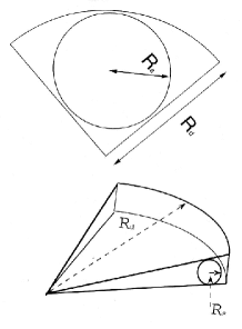
Figure 1: Upper part: A typical cone diagram for a wide angle galaxy catalog (e.g. CfA, SSRS, Perseus-Pisces). The depth is $R_{d}$. The effective depth is $R_{eff}$ and it corresponds to the radius of the maximum sphere fully contained in the sample volume ($R_{eff}\mathrel{\hbox to0.0pt{\lower 3.0pt\hbox{$\mathchar 536\relax$}\hss}\raise 2.0pt\hbox{$\mathchar 316\relax$}}R_{s}$). Bottom part: A typical cone diagram for a narrow angle galaxy catalog (e.g. LCRS, ESP). In this case $R_{eff}<<R_{d}$.

For example for a catalog with the limits in right ascension ($\alpha_{1}\leq\alpha\leq\alpha_{2}$) and declination ($\delta_{1}\leq\delta\leq\delta_{2}$) we have that

$$R_{eff}=\frac{R_{s}sin(\delta\theta/2)}{1+sin(\delta\theta/2)}$$ (20)

where $\delta\theta=min(\alpha_{2}-\alpha_{1},\delta_{2}-\delta_{1})$. In such a way we do not consider in the statistics the points for which a sphere of radius r is not fully included within the sample boundaries. Hence we do not make use of any weighting scheme with the advantage of not making any assumption in the treatment of the boundaries conditions. For this reason we have a smaller number of points and we stop our analysis at a smaller depth than that of other authors.

The reason why $\Gamma(r)$ (or $\xi(r)$ see in what follows) cannot be computed for $r>R_{eff}$ is essentially the following. When one evaluates the correlation function (or power spectrum) beyond $R_{eff}$, then one makes explicit assumptions on what lies beyond the sample’s boundary. In fact, even in absence of corrections for selection effects, one is forced to consider incomplete shells calculating $\Gamma(r)$ for $r>R_{eff}$, thereby implicitly assuming that what one does not find in the part of the shell not included in the sample is equal to what is inside (or other similar weighting schemes). In other words, the standard calculation introduces a spurious homogenization which we are trying to remove.

If one could reproduce via an analysis that uses weighting schemes, the correct properties of the distribution under analysis, it would be not necessary to produce wide angle survey, and from a single pencil beam deep survey it would be possible to study the entire matter distribution up to very deep scales. It is evident that this could not be the case. By the way, we have done a test on the homogenization effects of weighting schemes on artificial distributions as well as on real catalogs, finding that the flattening of the conditional density is indeed introduced owing to the weighting, and does not correspond to any real feature in the galaxy distribution $\!{}^{{\bf?}}$.

2.2 Standard analysis

At this point it is instructive to consider the behaviour of the standard correlation function $\xi(r)$. Coleman & Pietronero (1992) clarify some crucial points of the such an analysis, and in particular they discuss the meaning of the so-called ”correlation length” $\>r_{0}$ found with the standard approach $\!{}^{{\bf?}}$ $\!{}^{{\bf?}}$ and defined by the relation:

$$\xi(r_{0})=1$$ (21)

where

$$\xi(r)=\frac{<n(\vec{r_{i}})n(\vec{r_{i}}+\vec{r})>_{i}}{<n>^{2}}-1$$ (22)

is the two point correlation function used in the standard analysis. If the average density is not a well defined intrinsic property of the system, the analysis with $\xi(r)$ gives spurious results. In particular, if the system has fractal correlations, the average density is simply related to the sample size as shown by Eq.(15). In other words, it is meaningless to define the correlation length of the distribution by comparing the average correlation $<n(\vec{r_{i}})n(\vec{r_{i}}+\vec{r})>_{i}$ to the average density of the sample $<n>^{2}$, if the latter depends on the sample volume. The expression of the $\>\xi(r)$ for a fractal distribution is $\!{}^{{\bf?}}$

$$\xi(r)=((3-\gamma)/3)(r/R_{s})^{-\gamma}-1$$ (23)

where $\>R_{s}$ (the effective sample radius) is the radius of the spherical volume where one computes the average density from Eq. (15). From Eq. (23) it follows that: i.) the so-called correlation length $\>r_{0}$ (defined as $\>\xi(r_{0})=1$) is a linear function of the sample size $\>R_{s}$

$$r_{0}=((3-\gamma)/6)^{\frac{1}{\gamma}}R_{s}$$ (24)

and hence it is a quantity without any correlation meaning, but it is simply related to the sample size.

ii.) the amplitude of the $\xi(r)$ is:

$$A(R_{s})=((3-\gamma)/3)R_{s}^{\gamma}$$ (25)

iii.) $\>\xi(r)$ is a power law only for

$$((3-\gamma)/3)(r/R_{s})^{-\gamma}>>1$$ (26)

hence for $\>r\mathrel{\hbox to0.0pt{\lower 3.0pt\hbox{$\mathchar 536\relax$}\hss}\raise 2.0pt\hbox{$\mathchar 316\relax$}}r_{0}$: for larger distances there is a clear deviation from a power law behavior due to the definition of $\>\xi(r)$. This deviation, however, is just due to the size of the observational sample and does not correspond to any real change of the correlation properties. It is clear that if one estimates the exponent of $\xi(r)$ at distances $r\mathrel{\hbox to0.0pt{\lower 3.0pt\hbox{$\mathchar 536\relax$}\hss}\raise 2.0pt\hbox{$\mathchar 318\relax$}}r_{0}$, one systematically obtains a higher value of the correlation exponent due to the break of $\xi(r)$ in the log-log plot. This is actually the case for the analyses performed so far: in fact, usually, $\xi(r)$ is fitted with a power law in the range $0.5r_{0}\mathrel{\hbox to0.0pt{\lower 3.0pt\hbox{$\mathchar 536\relax$}\hss}\raise 2.0pt\hbox{$\mathchar 316\relax$}}r\mathrel{\hbox to0.0pt{\lower 3.0pt\hbox{$\mathchar 536\relax$}\hss}\raise 2.0pt\hbox{$\mathchar 316\relax$}}2r_{0}$, where we get an higher value of the correlation exponent. In particular, the usual estimation of this exponent by the $\xi(r)$ function leads to $\gamma\approx 1.7$, different from $\gamma\approx 1$ (corresponding to $D\approx 2$), that we found by means of the $\Gamma(r)$ analysis $\!{}^{{\bf?}}$.

2.3 Normalization of the average density in different surveys

We have already defined the luminosity factor which is associated to each VL sample. As long as the space and the luminosity density can be considered independent, the normalization of $\Gamma(r)$ in different VL samples can be simply done by dividing their amplitudes for the corresponding luminosity factors. Of course such a normalization is parametric, because it depends on the two parameters of the luminosity function $\delta$ and $M^{*}$ For a reasonable choice of these two parameters we find that the amplitude of the conditional and radial density matches quite well in different VL samples. In particular:

• (1) For CfA1, PP, ESP, LEDA and APM the parameters of the luminosity function are $\delta=-1.1$ and $M^{*}=-19.5$. All these surveys have been selected in the B-band, and hence the luminosity function is the same.

• (2) For SSRS1 the selection criteria have been chosen in the apparent diameter $d$, and hence we use the linear-diameter function, rather than the luminosity function for the normalization of the amplitude in different VL samples. We use the diameter function:

  $$N(D)dD=N_{0}\cdot exp(-\delta_{d}\cdot D)dD$$ (27)

  where $D$ is the absolute diameter (in Kpc), $\delta_{d}=0.109$ and $N_{0}$ is a constant $\!{}^{{\bf?}}$. The shape of this linear-diameter function is similar to the Schecther one for magnitudes.

• (3) Galaxies in LCRS have been measured in the $r$ band, so that we have used the luminosity function given by Schetman et al.(1996), i.e. a Schecther like function with parameters $\delta=-0.9$ and $M^{*}=-20.03$.

• (4) The two IRAS surveys have been measured in the near infrared. In this case we have normalized the amplitude of the density using the $IR$ luminosity function $\!{}^{{\bf?}}$.

We find that in all the cases (1)-(4) the density amplitude in the different VL samples match quite well (see Figs.2-3).

Figure 2: The spatial conditional average density $\Gamma^{*}(r)$ computed in some VL samples of Perseus-Pisces, CfA1, ESP and LEDA and normalized to the corresponding luminosity factor.

Figure 3: The spatial conditional average density $\Gamma^{*}(r)$ computed in some VL samples of APM, LCRS, SSRS1, IRAS $1.2Jy$ and normalized to the luminosity factor.

The main data of our correlation analysis are collected in Fig.4 (left part) in which we report the conditional density as a function of scale for the various catalogues. The relative position of the various lines is not arbitrary but it is fixed by the luminosity function, a part for the cases of IRAS and SSRS1 for which this is not possible. The properties derived from different catalogues are compatible with each other and show a power law decay for the conditional density from $1h^{-1}Mpc$ to $150h^{-1}Mpc$ without any tendency towards homogenization (flattening). This implies necessarily that the value of $r_{0}$ (derived from the $\xi(r)$ approach) will scale with the sample size $R_{s}$ as shown also from the specific data about $r_{0}$ of the various catalogues. The behaviour observed corresponds to a fractal structure with dimension $D\simeq 2$. (The data beyond $\sim 200h^{-1}Mpc$ have been obtained by measuring the radial density and are therefore weaker from a statistical point of view - see below) The smaller value of CfA1 was due to its limited size. An homogeneous distribution would correspond to a flattening of the conditional density which is never observed

Figure 4: Full correlation analysis for the various available redshift surveys in the range of distance $0.5\div 1000h^{-1}Mpc$. A reference line with slope $-1$ is also shown, that corresponds to fractal dimension $D=2$.

It is remarkable to stress that the amplitudes and the slopes of the different surveys match quite well. From this figure we conclude that galaxy correlations show very well defined fractal properties in the entire range $0.5\div 1000h^{-1}Mpc$ with dimension $D=2\pm 0.2$. Moreover all the surveys are in agreement with each other.

It is interesting to compare the analysis of Fig.4 with the usual one, made with the function $\xi(r)$, for the same galaxy catalogs. This is reported in Fig.5

Figure 5: Traditional analyses based on the function $\xi(r)$ of the same galaxy catalogs of the previous figure. The usual analysis is based on the a priori untested assumptions of analyticity and homogeneity. These properties are not present in the real galaxy distribution and the results appear therefore rather confusing. This lead to the impression that galaxy catalogs are not good enough and to a variety of theoretical problems like the galaxy-cluster mismatch, luminosity segregation, linear and non-linear evolution, etc.. This situation changes completely and becomes quite clear if one adopts the more general conceptual framework that is at the basis the previous figure

and, from this point of view, the various data the various data appear to be in strong disagreement with each other. This is due to the fact that the usual analysis looks at the data from the prospective of analyticity and large scale homogeneity (within each sample). These properties have never been tested and they are not present in the real galaxy distribution so the result is rather confusing (Fig.5). Once the same data are analyzed with a broader perspective the situation becomes clear (Fig.4) and the data of different catalogs result in agreement with each other. It is important to remark that analyses like those of Fig.5 have had a profound influence in the field in various ways: first the different catalogues appear in conflict with each other. This has generated the concept of not fair samples and a strong mutual criticism about the validity of the data between different authors. In the other cases the discrepancy observed in Fig.5 have been considered real physical problems for which various technical approaches have been proposed. These problems are, for example, the galaxy-cluster mismatch, luminosity segregation, the richness-clustering relation and the linear non-linear evolution of the perturbations corresponding to the ”small” or ”large” amplitudes of fluctuations. We can now see that all this problematic situation is not real and it arises only from a statistical analysis based on inappropriate and too restrictive assumptions that do not find any correspondence in the physical reality. It is also important to note that, even if the galaxy distribution would eventually became homogeneous at larger scales, the use of the above statistical concepts is anyhow inappropriate for the range of scales in which the system shows fractal correlations as those shown in Fig.4.

3 Radial density

In the previous sections we have discussed the methods that allow one to measure the conditional (average) density in real galaxy surveys. This statistical quantity is an average one, since it is determined by performing an average over all the points of the sample. We have discussed the robustness and the limits of such a measurement. We have pointed out that the estimate of the conditional density can be done up to a distance $R_{eff}$ which is of the order of the radius of the maximum sphere fully contained in the sample volume. This is because the conditional density must be computed only in spherical shells. This condition puts a great limitation to the volume studied, especially in the case of deep and narrow surveys, for which the maximum depth $R_{s}$ can be one order of magnitude, or more, than the effective depth $R_{eff}$.

We discuss here the measurement of the radial density in VL samples $\!{}^{{\bf?}}$. The determination of such a quantity allow us to extend the analysis of the space density well beyond the depth $R_{eff}$. The price to pay is that such a measurement is strongly affected by finite size spurious fluctuations, because it is not an average quantity. These finite size effects require a great caution $\!{}^{{\bf?}}$: the behaviour of statistical quantities (like the radial density and the counts of galaxies as a function of the apparent magnitude) that are not averaged out, present new and subtle problems.

3.1 Finite size effects and the behavior of the radial density

In this section we discuss the general problem of the minimal sample size which is able to provide us with a statistically meaningful information. For example, the mass-length relation for a fractal, which defines the fractal dimension, is

$$D=\lim_{r\rightarrow\infty}\frac{\log(N(<r))}{\log(r)}$$ (28)

However this relation is properly defined only in the asymptotic limit, because only in this limit the fluctuations of fractal structures are self-averaging. A fractal distribution is characterized by large fluctuations at all scales and these fluctuations determine the statistical properties of the structure. If the structure has a lower cut-off, as it is the case for any real fractal, one needs a ”very large sample” in order to recover the statistical properties of the distribution itself. Indeed, in any real physical problem we would like to recover the asymptotic properties from the knowledge of a finite portion of a fractal and the problem is that a single finite realization of a random fractal is affected by finite size fluctuations due to the lower cut-off.

In a homogeneous distribution we can define, in average, a characteristics volume associated to each particle. This is the Voronoi volume $\!{}^{{\bf?}}$ $v_{v}$ whose radius $\ell_{v}$ is of the order of the mean particle separation. It is clear that the statistical properties of the system can be defined only in volumes much larger than $v_{v}$. Up to this volume in fact we observe essentially nothing. Then one begins to include a few (strongly fluctuating) points, and finally, the correct scaling behavior is recovered (Fig.6).

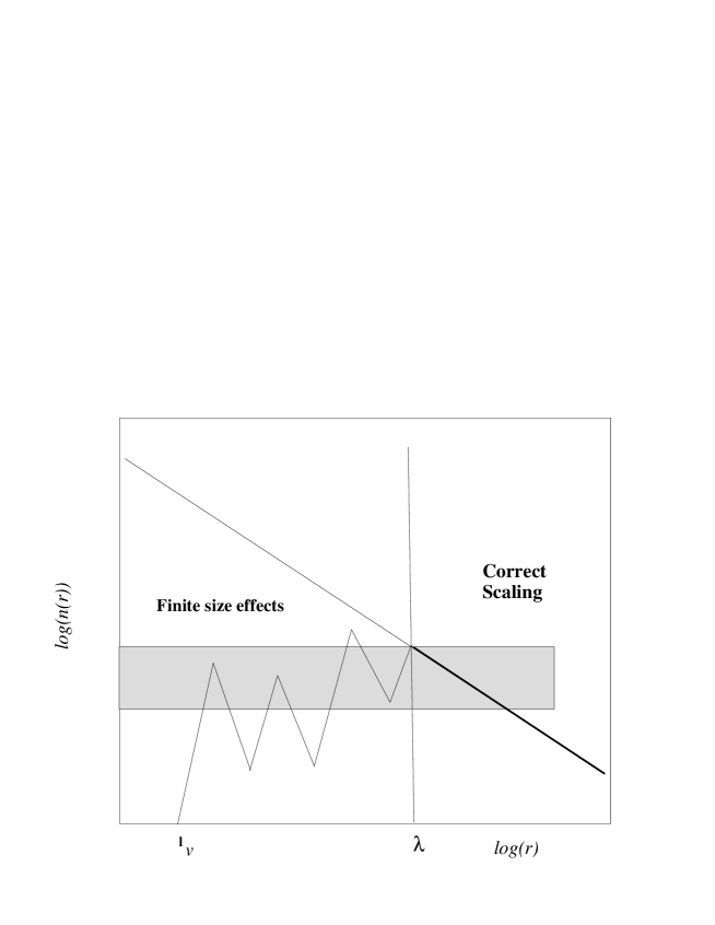
Figure 6: Behavior of the density computed from one point, in the case of a fractal distribution. At small distances below the average mean separation between neighbor galaxies, one finds no galaxies. Then the number of galaxies starts to grow, but this regime is strongly affected by finite size fluctuations. Finally the correct scaling region $r\approx\lambda$ is reached. In the intermediate region the density can be approximated roughly by a constant value. This leads to an apparent exponent $D\approx 3$. This exponent is not real but just due to the size effects.

For a Poisson sample consisting of $N$ particles inside a volume $V$ then the Voronoi volume is of the order

$$v_{v}\sim\frac{V}{N}$$ (29)

and $\ell_{v}\approx v_{v}^{1/3}$. In the case of homogeneous distributions, where the fluctuations have small amplitude with respect to the average density, one readily recovers the statistical properties of the system at small distances, say, $r\mathrel{\hbox to0.0pt{\lower 3.0pt\hbox{$\mathchar 536\relax$}\hss}\raise 2.0pt\hbox{$\mathchar 318\relax$}}5\ell_{v}$.

The case of fractal distribution is more subtle. Instead of the Voronoi length we can consider the average distance between nearest neighbors, but for clarity we proceed in the following way. Eq.13 gives the mass-length relation for a fractal. In this case, the prefactor $B$ is defined for spherical samples. If we have a sample consisting in a portion of a sphere characterized by a solid angle $\Omega$, we write

$$N(<R)=BR^{D}\frac{\Omega}{4\pi}\;.$$ (30)

In the case of a finite fractal structure, we have to take into account the statistical fluctuations. We can identify two basic kinds of fluctuations: the first ones are intrinsic $f(R)$ and are due to the highly fluctuating nature of fractal distributions while the second ones, $P(R)$, are Poissonian fluctuations. Concerning the first ones, one has to consider that the mass-length relation is a convolution of fluctuations which are present at all scales. For example one encounters, at any scale, a large scale structure and then a huge void: these fluctuations affect the power law behavior of $N(<R)$. We can quantify these effects as a modulating term around the expected average given by Eq.30. Therefore, in the observations from a single point ”i” we have

$$[N(<R)]_{i}=BR^{D}\frac{\Omega}{4\pi}\cdot f_{\Omega}(R,\delta\Omega)\;.$$ (31)

In general it is more useful to focus on the behaviour of a local quantity (as the number of points in shells) rather than an integrated one. However for the purpose of the present discussion the approximation given by Eq.31 is rather good. This equation shows that the amplitude of $N(<r)$ is related to the amplitude of the intrinsic fluctuations and not only to the lower cut-off $B$. The amplitude of the modulating term is small, compared with the expected value of $N(<R)$

$$\sqrt{|f(R)|^{2}}<BR^{D}\frac{\Omega}{4\pi}\;.$$ (32)

In general this fluctuating term depends on the direction of observation $\Omega$ and on the solid angle of the survey $\delta\Omega$ so that $f(R)=f_{\Omega}(R,\delta\Omega)$. If we have a spherical sample we get

$$\frac{1}{4\pi}\sum_{\Omega}f_{\Omega}(R,\delta\Omega)=f_{4\pi}(R)\;.$$ (33)

In general we expect that $f_{\Omega}(R,\delta\Omega)>f_{4\pi}(R)$, so that larger is the solid angle and smaller is the effect this term. If we perform the ensemble average of this fluctuating term we can smooth out its effect and we have then

$$\langle f_{4\pi}(R)\rangle_{i}=1$$ (34)

where the average $\langle....\rangle_{i}$ refers to all the occupied points in the sample. In such a way the conditional density, averaged over all the points of the sample, has a single power law behavior. We stress that according to Eq.31 the fluctuations in the integrated number of points in a fractal, are proportional to the number of points itself, rather than to the root mean square as in a poissonian distribution. In general $\!{}^{{\bf?},{\bf?},{\bf?},{\bf?}}$ it is possible to characterize these intrinsic fluctuations as log-periodic oscillations in the power law behavior. By performing an ensemble average as in Eq.34 these oscillations can be smoothed out. However for the purpose of the present paper, we limit our discussion to the approximation of Eq.31, without entering in more details.

The second $P(R)$ term is an additive one, and it takes into account spurious finite size fluctuations is simply due to shot noise. In this case we have that

$$\sqrt{|P(R)|^{2}}>BR^{D}\frac{\Omega}{4\pi}\;\;\;\mbox{if}\;\;\;R<\lambda\;$$ (35)

while $P(R)\approx 0$ for $R\mathrel{\hbox to0.0pt{\lower 3.0pt\hbox{$\mathchar 536\relax$}\hss}\raise 2.0pt\hbox{$\mathchar 318\relax$}}\lambda$. The ensemble average is, again, expected to be

$$\langle P(R)\rangle_{i}=0\;.$$ (36)

This term becomes negligible if the shot noise fluctuations are small: for example, if

$$[N(<R)]_{i}>10\sqrt{[N(<R)]_{i}}\;.$$ (37)

From this condition and Eq.31 we can have a condition on $\lambda$ (neglecting the effect of $f(R)$):

$$\langle\lambda\rangle\sim\left(10^{2}\frac{4\pi}{B\Omega}\right)^{\frac{1}{D}}$$ (38)

The minimal statistical length $\lambda$ is an explicit function of the prefactor $B$ and of the solid angle of the survey $\Omega$. This scale is a lower limit for the scaling region of the distribution: the effect of intrinsic fluctuations, described by $f(R)$, which are in general non negligible, can modulate the distance at which the scaling region is reached. This length depends also, but weakly, on the particular morphological features of the sample. Therefore it is important to stress that Eq.38 gives an order of magnitude for $\langle\lambda\rangle$, where we intend the average value over all the possible directions of observations. In different directions one can have different values for $\langle\lambda\rangle$, because of the effect of $f(r)$.

In the case of real galaxy catalogs we have to consider the luminosity selection effects. In a VL sample, characterized by an absolute magnitude limit $M_{lim}$, the mass-length relation Eq.30, can be generalized as

$$N(R,M_{lim})=BR^{D}\frac{\Omega}{4\pi}\psi(M_{lim})$$ (39)

where $\psi(M_{lim})$ is the probability that a galaxy has an absolute magnitude brighter than $M_{lim}$

$$0<\psi(M_{lim})=\frac{\int_{-\infty}^{M_{lim}}\phi(M)dM}{\Psi(\infty)}<1$$ (40)

where $\phi(M)$ is the Schecther luminosity function (normalized to unity) and $\Psi(\infty)$ is the normalizing factor

$$\Psi(\infty)=\int_{-\infty}^{M_{min}}\phi(M)dM$$ (41)

where $M_{min}$ is the fainter absolute magnitude surveyed in the catalog (usually $M_{min}\approx-10\div-11$).

It is possible to compute the intrinsic prefactor $B$ from the knowledge of the conditional density $\Gamma(r)$ (Eq.16 $\!{}^{{\bf?},{\bf?}}$) computed in the VL samples and normalized for the luminosity factor (Eq.40). In the various VL subsamples of Perseus-Pisces, CfA1, and other redshift surveys we find that

$$B\approx 10\div 15(h^{-1}Mpc)^{-D}$$ (42)

depending on the parameters of the Schecther function $M^{*}$ and $\delta$. From Eq.38, Eq.39 and Eq.42 we obtain for a typical volume limited sample with $M_{lim}\approx M^{*}$,

$$\langle\lambda\rangle\approx\frac{(20\div 60)h^{-1}Mpc}{\Omega^{\frac{1}{D}}}\;.$$ (43)

This is the value of the minimal statistical length that we use in what follows. In Tab. 1 we report the value of $\lambda$ for several redshift surveys. While in the case of CfA1, SSRS1, PP, LEDA and ESP we have checked that there is a reasonable agreement with this prediction, the CfA2 and SSRS2 redshift surveys are not sill published and hence in these cases we can predict the value of $\lambda$.

Survey	$\Omega(sr)$	$\lambda(h^{-1}Mpc)$
CfA1	1.8	15
CfA2 (North)	1.3	20
SSRS1	1.75	15
SSRS2	1.13	20
PP	1	40
LEDA	2 $\pi$	10
IRAS	2 $\pi$	15
ESP	0.006	300

Table 1: The minimal statistical length $\lambda$ for several redshift surveys

Given the previous discussion, we can now describe in a very simple way the behavior of $[N(<r)]_{i}$, i.e. the mass length relation measured from a generic point ”i”. Given a sample with solid angle $\Omega$, we can approximate the effect of the intrinsic and shot noise fluctuations in the following way:

$$(N(<r))_{i}=B_{1}r^{3}\;\;\;\mbox{if}\;\;r\mathrel{\hbox to0.0pt{\lower 3.0pt\hbox{$\mathchar 536\relax$}\hss}\raise 2.0pt\hbox{$\mathchar 316\relax$}}\lambda$$ (44)

i.e. the density is constant up to $\lambda$, while

$$(N(<r))_{i}=Br^{D}\;\;\;\mbox{if}\;\;r\mathrel{\hbox to0.0pt{\lower 3.0pt\hbox{$\mathchar 536\relax$}\hss}\raise 2.0pt\hbox{$\mathchar 318\relax$}}\lambda$$ (45)

so that by the condition of continuity at $\lambda$ we have

$$B_{1}=\frac{B}{\lambda^{3-D}}$$ (46)

This simple approximation is very useful in the following discussion, especially for the number counts.

To clarify the effects of the spatial inhomogeneities and finite effects we have studied the behavior of the galaxy radial (number) density in the VL samples, i.e. the behavior of (using Eq.39 and Eq.31)

$$n_{VL}(r)=\frac{N(<r)}{V(r)}=\frac{3}{4\pi}Br^{D-3}\psi(M_{lim})\cdot f_{\Omega}(r,\delta\Omega)$$ (47)

One expects that, if the distribution is homogeneous the density is constant, while if it is fractal it decays as power law.

When one computes the conditional average density, one indeed performs an average over all the points of the survey. In particular, as we have already discussed, we limit our analysis to a size defined by the radius of the maximum sphere fully contained in the sample volume, and we do not make use any treatment of the sample boundaries. On the contrary Eq.47 is computed only from a single point, the origin. This allows us to extend the study of the spatial distribution up to very deep scales. The price to pay is that this method is strongly affected by statistical fluctuations and finite size effects.

The effect of the finite size spurious fluctuations for a fractal distribution is shown Fig.6: at small distances one finds almost no galaxies because we are below the average separation between neighbor galaxies $\ell$. Then the number of galaxies starts to grow, but this regime is strongly affected by finite size fluctuations. Finally the correct scaling region $r\approx\lambda$ is reached. This means, for example, that if one has a fractal distribution, there is first a raise of the density, due to finite size effects and characterized by strong fluctuations, because no galaxies are present before a certain characteristic scale. Once one enters in the correct scaling regime for a fractal the density starts to decay as a power law. So in this regime of raise and fall with strong fluctuations there is a region in which the density can be approximated roughly by a constant value. This leads to an apparent exponent $D\approx 3$, so that the integrated number grows as $N(<r)\sim r^{3}$. This exponent is therefore not a real one but just due to finite size fluctuations. Of course, depending on the survey orientation in the sky, one can get an exponent larger or smaller than $3$, but in general this is the more frequent situation (see below). Only when a well defined statistical scaling regime has been reached, i.e. for $r>\lambda$, one can find the genuine scaling properties of the structure, otherwise the behavior is completely dominated by spurious finite size effects (for seek of clarity in this discussion we do not consider the effect of $f(r)$ in Eq.31)

The question of the difference between the integration from the origin (radial density) and correlation properties averaged over all points lead us to a subtle problem of asymmetric fluctuations in a fractal structure. From our discussion, exemplified by Fig.6, the region between $\ell$ and $\lambda$ corresponds to an underdensity with respect to the real one. However we have also showed that for the full correlation averaged over all the points, as measured by $\Gamma(r)$, the correct scaling is recovered at distances appreciably smaller than $\lambda$. This means that in some points one should observe an overdensity between $\ell$ and $\lambda$. However, given the intrinsic asymmetry between filled and empty regions in a fractal, only very few points show the overdensity (a fractal structure is asymptotically dominated by voids). These few points nevertheless have, indeed, an important effect on the average values of the correlations. This means that, in practice, a typical points shows an underdensity up to $\lambda$ as shown in Fig.6. The full averages instead converge at much shorter distances. This discussion shows the peculiar and asymmetric nature of finite size fluctuations in fractals as compared to the symmetric Poissonian case. For homogeneous distribution$\!{}^{{\bf?}}$ the situation is in fact quite different. Below the Voronoi length $\ell_{v}$ there are finite size fluctuations, but for distances $r\mathrel{\hbox to0.0pt{\lower 3.0pt\hbox{$\mathchar 536\relax$}\hss}\raise 2.0pt\hbox{$\mathchar 318\relax$}}(2\div 4)\ell_{v}$ the correct scaling regime is readily found for the density. In this case the finite size effects do not affect too much the properties of the system because a Poisson distribution is characterized by small amplitude fluctuations.

As an example, we show the behaviour of the radial density in the Perseus-Pisces redshift survey (PPRS). We have computed the $n(r)$ in the various VL samples of PPRS, and we show the results in Fig.7. In the less deeper VL samples (VL70, VL90) the density does not show any smooth behavior because in this case the finite size effects dominate the behavior as the distances involved are $r<\lambda$ (Eq.43). At about the same scales we find a very well defined power law behavior by the correlation function analysis. In the deeper VL samples (VL110, VL130) a smooth behavior is reached for distances larger than the scaling distance ($\Omega=0.9\,sr$) $r\approx\lambda\sim 50h^{-1}Mpc$. The fractal dimension is $D\approx 2$ as one measures by the correlation function.

Figure 7: The spatial density $n(r)$ computed in the VL sample cut at $70,90,110,130h^{-1}Mpc$ . In the case of VL70 and VL90 the density is dominated by large fluctuations and it has not reached the scaling regime. In the samples VL110 and VL130 the density is dominated by large fluctuations only at small distances, while at larger distances, after the Perseus Pisces chain at $50h^{-1}Mpc$, a very well defined power law behavior is shown, with the same exponent of the correlation function (i.e. $D=2$)

For relatively small volumes it is possible to recover the correct scaling behavior for scales of order of $\ell$ (instead of $\sim 10\ell$) by averaging over several samples or, as it happens in real cases, over several points of the same sample when this is possible. Indeed, when we compute the correlation function we perform an average over all the points of the system even if the VL sample is not deep enough to satisfy the condition expressed by Eq.43. In this case the lower cut-off introduces a limit in the sample statistics $\!{}^{{\bf?}}$.

The case of LCRS and ESP are discussed in detail in Sylos Labini et al.(1997) and the results are shown in Fig.4

3.2 Pencil beams

Deep ”pencil beams” surveys cover in general very narrow angular size ($\sim 1^{\circ}$) and extend to very deep depths ($z\mathrel{\hbox to0.0pt{\lower 3.0pt\hbox{$\mathchar 536\relax$}\hss}\raise 2.0pt\hbox{$\mathchar 318\relax$}}0.2$). These narrow shots through deep space provide a confirmation of strong inhomogeneities in the galaxy distribution.

One of the most discussed results obtained from pencil-beams surveys has been the claimed detection of a typical scale in the distribution of galaxy structures, corresponding to a characteristic separation of $128h^{-1}Mpc$ $\!{}^{{\bf?}}$. However in the last five years several other surveys, in different regions of the sky, do not find any evidence for such a periodicity. In particular, Bellanger & De Lapparent $\!{}^{{\bf?}}$, by analyzing a sample of 353 galaxies in the redshift interval $0.1\mathrel{\hbox to0.0pt{\lower 3.0pt\hbox{$\mathchar 536\relax$}\hss}\raise 2.0pt\hbox{$\mathchar 316\relax$}}z\mathrel{\hbox to0.0pt{\lower 3.0pt\hbox{$\mathchar 536\relax$}\hss}\raise 2.0pt\hbox{$\mathchar 316\relax$}}0.5$, concluded that these new data contain no evidence for a periodic signal on a scale of $128h^{-1}Mpc$. Moreover they argue that the low sampling rate of $\!{}^{{\bf?}}$ is insufficient for mapping the detailed large-scale structure and it is the real origin of the apparent periodicity.

On the other hand, Willmer et al.(1994) detect four of the five nearest peaks of the galaxies detected by $\!{}^{{\bf?}}$, because their survey is contiguous to that of $\!{}^{{\bf?}}$, in the sky region near the north Galactic pole. Moreover Ettori et al.(1996) in a survey oriented in three small regions around the South Galactic Pole do not find any statistically periodic signal distinguishable from noise. Finally Cohen et al.$\!{}^{{\bf?}}$ by analyzing a sample of 140 objects up to $z\sim 0.8$, find that there is no evidence for periodicity in the peak redshifts.

In a pencil-beam survey one can study the behavior of the linear density along a tiny but very long cylinder. The observed galaxy distribution corresponds therefore to the intersection of the full three dimensional galaxy distribution with one dimensional cylinder $\!{}^{{\bf?}}$. In this case, from the law of codimension additivity $\!{}^{{\bf?},{\bf?}}$, one obtains that the fractal dimension of the intersection is given by

$$D_{I}=D+d_{pc}-d\approx D+1-3\approx 0$$ (48)

where $D$ is the galaxy distribution fractal dimension, embedded in a $d=3$ Euclidean space, and $d_{pc}=1$ is the dimension of the pencil beam survey. This means that the set of points visible in a randomly oriented cylinder has dimension $D_{I}\approx 0$. In such a situation the power law behavior is no longer present and the data should show a chaotic, featureless nature strongly dependent on the beam orientation. If the galaxy distribution becomes instead homogeneous above some length, shorter than the pencil beam depth, one has the regular situation $D_{I}=1$ and a well defined density must be observed.

We stress that in any of the available pencil beams surveys, one can detect tendency towards an homogeneous distribution. Rather, all these surveys show a very fluctuating signal, characterized by the presence of galaxy structures. Some authors $\!{}^{{\bf?}}$ claim to detect the end greatness (i.e. that the galaxy structures in the deep pencil beams are not so different from those seen in nearby sample - as the Great Wall), or that $\!{}^{{\bf?}}$ the dimension of voids does not scale with sample size, by the visual inspection of these surveys. However one should consider in these morphological analyses, that one is just looking at a convolution of the survey geometry, which in general are characterized by very narrow solid angles, and large scale structures, and that in such a situation, a part from very favorable cases, one may detect portions of galaxy structures (or voids).

Finally we note that if the periodicity would be present, the amplitude of the different peaks is very different from each other, and an eventual transition to homogeneity in a periodic lattice, should be, for example, ten times the lattice parameter, i.e. $\mathrel{\hbox to0.0pt{\lower 3.0pt\hbox{$\mathchar 536\relax$}\hss}\raise 2.0pt\hbox{$\mathchar 318\relax$}}1000h^{-1}Mpc$ !

4 Number Counts

The most complete information about galaxy distribution comes from the full three dimensional samples, while the angular catalogs have a poorer qualitative information, even if usually they contain a much larger number of galaxies. However, one of the most important tasks in observational astrophysics, is the determination of the $\log N-\log S$ relation for different kind of objects: galaxies in the various spectral band (from ultraviolet to infrared), radio-galaxies, Quasars, X-ray sources and $\gamma$-ray bursts. This relation gives the number $N(S)$ (integral or differential) of objects, for unit solid angle, with apparent flux (larger than a certain limit) $S$. The determination of such a quantity avoids the measurements of the distance, which is always a very complex task. However we show in the following that the behavior of the $\log N-\log S$ is strongly biased by some statistical finite size effects due to small scale fluctuations.

The counts of galaxies as a function of the apparent magnitude are determined from the Earth only, and hence it is not possible to make an average over different observers. As we have already discussed in the previous section, this kind of measurement is affected by intrinsic fluctuations that are not smoothed out at any scale. Moreover at small scale there are finite size effects which may seriously perturb the behavior of the observed counts. Following the simple argument about the behaviour of the radial density we have presented in the previous section, we consider here the problem of the galaxy-number counts.

We present in this section a new interpretation of this basic relation at the light of the highly inhomogeneity nature of galaxy distribution, and we show its compatibility with the behavior of counts of galaxies in different frequency bands, radiogalaxies, Quasars and X-ray sources. Our conclusion is that the counts of all these different kind of objects are compatible with a fractal distribution of visible matter up to the deepest observable scale.

4.1 Galaxy number counts data

Historically $\!{}^{{\bf?},{\bf?}}$ the oldest type of data about galaxy distribution is given by the relation between the number of observed galaxies $N(>S)$ and their apparent brightness $S$. It is easy to show that, under very general assumptions one gets (see Sec.4.2)

$$N(>S)\sim S^{-\frac{D}{2}}$$ (49)

where $D$ is the fractal dimension of the galaxy distribution. Usually this relation is written in terms of the apparent magnitude $m$ ($S\sim 10^{-0.4m}$ - note that bright galaxies correspond to small $m$). In terms of $m$, Eq.49 becomes

$$\log N(<m)\sim\alpha m$$ (50)

with $\alpha=D/5$ $\!{}^{{\bf?},{\bf?}}$. Note that $\alpha$ is the coefficient of the exponential behavior of Eq.50 and we call it ”exponent” even though it should not be confused with the exponents of power law behaviors. In Fig.8

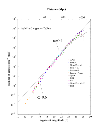
Figure 8: The galaxy number counts in the $B$-band, from several surveys. In the range $12\mathrel{\hbox to0.0pt{\lower 3.0pt\hbox{$\mathchar 536\relax$}\hss}\raise 2.0pt\hbox{$\mathchar 316\relax$}}m\mathrel{\hbox to0.0pt{\lower 3.0pt\hbox{$\mathchar 536\relax$}\hss}\raise 2.0pt\hbox{$\mathchar 316\relax$}}19$ the counts show an exponent $\alpha\approx 0.6\pm 0.1$, while in the range $19\mathrel{\hbox to0.0pt{\lower 3.0pt\hbox{$\mathchar 536\relax$}\hss}\raise 2.0pt\hbox{$\mathchar 316\relax$}}m\mathrel{\hbox to0.0pt{\lower 3.0pt\hbox{$\mathchar 536\relax$}\hss}\raise 2.0pt\hbox{$\mathchar 316\relax$}}28$ the exponent is $\alpha\approx 0.4$. The solid line is computed from the determination of the amplitude of the conditional density at small scale, the fractal dimension $D=2.2$, and from the knowledge of the luminosity function. The distance is computed for a galaxy with $M=-16$ and we have used $H_{0}=75kmsec^{-1}Mpc^{-1}$.

we have collected all the recent observations of $N(<m)$ versus $m$ in the $B$-spectral-band $m_{B}$ $\!{}^{{\bf?},{\bf?},{\bf?},{\bf?},{\bf?},{\bf?},{\bf?}}$. At bright and intermediate magnitudes ($\>12\mathrel{\hbox to0.0pt{\lower 3.0pt\hbox{$\mathchar 536\relax$}\hss}\raise 2.0pt\hbox{$\mathchar 316\relax$}}m_{B}\mathrel{\hbox to0.0pt{\lower 3.0pt\hbox{$\mathchar 536\relax$}\hss}\raise 2.0pt\hbox{$\mathchar 316\relax$}}18$), corresponding to small redshift ($\>z<0.2$), one obtains $\>\alpha\approx 0.6$, while from $m_{B}\sim 19$ up to $m_{B}\sim 28$ the counts are well fitted by a smaller exponent with $\alpha\approx 0.4$. The usual interpretation $\!{}^{{\bf?},{\bf?},{\bf?},{\bf?},{\bf?}}$ is that $\alpha\approx 0.6$ corresponds to $D\approx 3$ consistent with homogeneity, while at large scales galaxy evolution and space time expansion effects are invoked to explain the lower value $\alpha\approx 0.4$. On the basis of the previous discussion of the VL samples, this interpretation is untenable. In fact, we know for sure that, at least up to $\sim 150h^{-1}Mpc$ there are fractal correlations, as we have discussed in the previous sections, so one would eventually expect the opposite behavior. Namely small value of $\alpha\approx 0.4$ (consistent with $D\approx 2$) at small scales followed by a crossover to an eventual homogeneous distribution at large scales ($\alpha\approx 0.6$ and $D\approx 3$).

The situation is therefore similar in the different spectral bands. The puzzling behavior of the GNC represents an important apparent contradiction we find in the data analysis. We argue here that this apparently contradictory experimental situation can be fully understood on the light of the small scale effects in the space distribution of galaxies. For example a fractal distribution is non analytic in every occupied point: it is not possible to define a meaningful average density because we are dealing with intrinsic fluctuations which grow with as the scale of the system itself. This situation is qualitatively different from an homogeneous picture, in which a well defined density exists, and the fluctuations represent only small amplitude perturbations. The nature of the fluctuations in these two cases is completely different, and for fractals the fluctuations themselves define all the statistical properties of the distribution. This concept has dramatic consequences in the following discussion as well as in the determination of various observable quantities, such as the amplitude of the two point angular correlation function. It is worth to notice that the small scale effects are usually neglected in the study of fractal structures because one can generate large enough (artificial) structures to avoid these problems. In Astrophysics the data are instead intrinsically limited and a detailed analysis of finite size effects is very important. We discuss the problems of finite size effects in the determination of the asymptotic properties of fractal distributions, considering explicitly the problems induced by the lower cut-off.

4.2 Galaxy counts: basic relations

We briefly introduce some basic relations which are useful later. We can start by computing the expected GNC in the simplest case of a magnitude limited (ML) sample. A ML sample is obtained by measuring all the galaxies with apparent magnitude brighter than a certain limit $m_{lim}$. In this case we have (for $m<m_{lim}$)

$$N(<m)=B\Phi(\infty)10^{\frac{D}{5}m}$$ (51)

where

$$\Phi(\infty)=\int_{-\infty}^{\infty}\phi(M)10^{-\frac{D}{5}(M+25)}dM\;.$$ (52)

We consider now the case of a volume limited (VL) sample. A VL sample consists of every galaxy in the volume which is more luminous than a certain limit, so that in such a sample there is no incompleteness for an observational luminosity selection effect $\!{}^{{\bf?},{\bf?}}$. Such a sample is defined by a certain maximum distance $R$ and an absolute magnitude limit given by:

$$M_{lim}=m_{lim}-5\log_{10}R-25-A(z)$$ (53)

($m_{lim}$ is the survey apparent magnitude limit). By performing the calculations for the number-magnitude relation, we obtain

$$N(<m)=A(m)\cdot 10^{\frac{D}{5}m}+C(m)$$ (54)

where $A(m)$ is

$$A(m)=B\int_{M(m)}^{M_{lim}}\phi(M)10^{-\frac{D}{5}(M+25)}dM$$ (55)

and $M(m)$ is given by $M(m)=m-5\log(R)-25$, and it is a function of $m$. The second term is

$$C(m)=BR^{D}\int_{-\infty}^{M(m)}\phi(M)dM\;.$$ (56)

This term, as $A(m)$, depends on the VL sample considered. We assume a luminosity function with a Schecther shape. For $M(m)\mathrel{\hbox to0.0pt{\lower 3.0pt\hbox{$\mathchar 536\relax$}\hss}\raise 2.0pt\hbox{$\mathchar 318\relax$}}M^{*}$ we have that $C(m)\approx 0$, and $A(m)$ is nearly constant with $m$. This happens in particular for the deeper VL samples for which $M_{lim}\sim M^{*}$. For the less deeper VL ($M_{lim}>M^{*}$) samples these terms can be considered as a deviation from a power law behavior only for $m\rightarrow m_{lim}$. If one has $\phi(M)=\delta(M-M_{0})$ then it is simple to show that $\log(N(<m))\sim(D/5)m$ also in each VL sample.

4.3 Galaxy counts in redshift surveys

We have studied the GNC in the Perseus-Pisces redshift survey $\!{}^{{\bf?}}$ in order to clarify the role of spatial inhomogeneities and finite size effects. In the previous sections we have analyzed the spatial properties of galaxy distribution in this sample by measuring the conditional (average) density and the radial density. Let us briefly summarize our main results.

When one computes the conditional average density, one indeed performs an average over all the points of the survey. On the contrary the radial density is computed only from a single point, the origin. This allows us to extend the study of the spatial distribution up to very deep scales: the price to pay is that this method is strongly affected by statistical fluctuations and finite size effects. Analogously, when one computes $N(<m)$, one does not perform an average but just counts the points from the origin. As in the case of the radial density $n(r)$ also $N(<m)$ is strongly affected by statistical fluctuations due to finite size effects. as well as intrinsic oscillations that are not smoothed out. We are now able to clarify how the behavior of $N(<m)$, and in particular its exponent, are influenced by these effects.

We show in Fig.9,

Figure 9: $(a)$ The Number counts $N(<m)$ for the VL sample VL60. The slope is $\alpha\approx 0.6$. In this case occurs a flattening for $m\rightarrow m_{lim}$. $(b)$ The Number counts $N(<m)$ for the VL sample VL110. The slope is $\alpha\approx 0.4$, a part from the initial fast growth due to weak statistics. This behavior corresponds to a well defined define power law behavior of the density with exponent $D\approx 5\alpha\approx 2$.

and Fig.10

Figure 10: The Number counts $N(<m)$ for the whole magnitude limit sample. The slope is $\alpha\approx 0.6$ and it is clearly associated only to fluctuations in the spatial distribution rather than to a real homogeneity in space.

the behavior of $N(<m)$ respectively for the various VL samples and for the whole magnitude limit sample. In VL60 there are very strong inhomogeneities in the behavior of $n(r)$ (see Fig.7) and these are associated with a slope $\alpha\approx 0.6$ for the GNC. (The flattening for $m\rightarrow m_{lim}$ is just due to a luminosity selection effect that is explained in Sec.4.2). For VL110 the behavior of the density is much more regular and smooth, so that it shows indeed a clear power law behavior. Correspondingly the behavior of $N(<m)$ is well fitted by $\alpha\approx 0.4$. Finally the whole magnitude limit sample is again described by an exponent $\alpha\approx 0.6$.

We have now enough elements to describe the behavior of the GNC. The first point is that the exponent of the GNC is strongly related to the space distribution. Indeed, what has never been taken into account before is the role of finite size effects $\!{}^{{\bf?}}$. The behavior of the GNC is determined by a convolution of the space density and the luminosity function, and the space density enters in the GNC as an integrated quantity. The problem is to consider the correct space density in the interpretation of data analysis. In fact, if the density has a very fluctuating behavior in a certain region of length scale, as in the case shown in Fig.7, its integral over this range of length scales is almost equivalent to a flat one. This can be seen also in Fig.6: at small distances one finds almost no galaxies because one is below the mean minimum separation between neighbor galaxies. Then the number of galaxies starts to grow, but this regime is strongly affected by finite size fluctuations. Finally the correct scaling region $r\approx\lambda$ is reached. This means for example that if one has a fractal distribution, there is first a raise of the density, due to finite size effects and characterized by strong fluctuations, because no galaxies are present before a certain characteristic scale. Once one enters in the correct scaling regime for a fractal the density becomes to decay as a power law. So in this regime of raise and fall with strong fluctuations there is a region in which the density can be approximated roughly by a constant value. This leads to an apparent exponent $D\approx 3$, so that the integrated number grows as $N(<r)\sim r^{3}$ and it is associated in terms of GNC, to $\alpha\approx 0.6$ (Fig.11).

Figure 11: The number counts $N(<m)$ together with the behavior of the space density. At small scale the density is characterized by having strong fluctuations which lead to a slope $\alpha\approx 0.6$. This is clearly associated only to fluctuations in the spatial distribution rather than to a real homogeneity in space. At larger scales (faint end) the correct scaling behavior is recovered and $\alpha=D/5$.

This exponent is therefore not a real one but just due to finite size fluctuations. Only when a well defined statistical scaling regime has been reached, i.e. for $r>\lambda$, one can find the genuine scaling properties of the structure, otherwise the behavior is completely dominated by spurious finite size effects. In the VL samples where $n(r)$ scales with the asymptotic properties (Fig.9) the GNC grows also with the right exponent ($\alpha=D/5$).

If we now consider instead the behavior of the GNC in the whole magnitude limit (hereafter ML) survey, we find that the exponent is $\alpha\approx 0.6$ (Fig.10). This behavior can be understood by considering that at small distances, well inside the distance $\lambda$ defined by Eq.43, the number of galaxies present in the sample is large because there are galaxies of all magnitudes. Hence the majority of galaxies correspond to small distances ($r<\lambda$) and the distribution has not reached the scaling regime in which the statistical self-averaging properties of the system are present. For this reason in the ML sample the finite size fluctuations dominate completely the behavior of the GNC. Therefore this behavior in the ML sample is associated with spurious finite size effects rather than to real homogeneity. We discuss in a more quantitative way the behavior in ML surveys later.

4.4 Test on finite size effects: the average $N(<m)$

To prove that the behavior found in Fig.10, i.e. that the exponent $\alpha\approx 0.6$ is connected to large fluctuations due to finite size effects in the space distribution and not to real homogeneity, we have done the following test. We have adopted the same procedure used for the computation of the correlation function, i.e. we make an average for $N(<m)$ from all the points of the sample rather than counting it from the origin only.

To this aim we have considered a VL sample with $N$ galaxies and we have built $N$ independent flux-limited surveys in the following way. We consider each galaxy in the sample as the observer, and for each observer we have computed the apparent magnitudes of all the other galaxies. To avoid any selection effect we consider only the galaxies which lie inside a well defined volume around the observer. This volume is defined by the maximum sphere fully contained in the sample volume with the observer as a center.

Moreover we have another selection effect due to the fact that our VL sample has been built from a ML survey done with respect to the origin. To avoid this incompleteness we have assigned to each galaxy a constant magnitude $M$. In fact, our aim is to show that the inhomogeneity in the space distribution plays the fundamental role that determines the shape of the $N(<m)$ relation, and the functional form of the luminosity function enters in Eq.55 only as an overall normalizing factor.

Once we have computed $N_{i}(<m)$ from all the points $i=1,..,N$ we then compute the average. We show in Fig.12

Figure 12: Left panel The average $N(<m)$ in the VL sample VL60. The squares crosses refer to the average $N(<m)$ computed assigning to all the galaxies the same absolute magnitude $M_{0}=M^{*}$. The reference line has a slope $\alpha=0.4$. Right panel The average $N(<m)$ in the VL sample VL110. The squares crosses refer to the average $N(<m)$ computed assigning to all the galaxies the same absolute magnitude $M_{0}=M^{*}$. The reference line has a slope $\alpha=0.4$

the results for VL60 and VL110: a very well defined exponent $\alpha=D/5\approx 0.4$ is found in both cases. This is in fully agreement with the average space density (the conditional average density $\Gamma(r)$) that shows $D\approx 2$ in these VL samples.

4.5 Behavior of galaxy counts in magnitude limited samples

We are now able to clarify the problem of ML catalogs. Suppose to have a certain survey characterized by a solid angle $\Omega$ and we ask the following question: up to which apparent magnitude limit $m_{lim}$ we have to push our observations to obtain that the majority of the galaxies lie in the statistically significant region ($r\mathrel{\hbox to0.0pt{\lower 3.0pt\hbox{$\mathchar 536\relax$}\hss}\raise 2.0pt\hbox{$\mathchar 318\relax$}}\lambda$) defined by Eq.43. Beyond this value of $m_{lim}$ we should recover the genuine properties of the sample because, as we have enough statistics, the finite size effects self-average. From the previous condition for each solid angle $\Omega$ we can find an apparent magnitude limit $m_{lim}$ so that finally we are able to obtain $m_{lim}=m_{lim}(\Omega)$ in the following way.

In order to clarify the situation, we can now compute the expected value of the counts if we use the approximation for the behavior of the mass-length relation given by Eqs.44-46. Suppose, for seek of clarity, also that $\phi(M)=\delta(M-M_{o})$, with $M_{o}=-19$. We define

$$\lambda=10^{0.2(m_{\lambda}-M-25)}$$ (57)

where $\lambda$ is given by Eq.43. Then the differential counts are given by

$$\left(\frac{dN}{dm}\right)_{i}=\frac{\log_{e}10}{5}3B_{1}\cdot 10^{\frac{3}{5}m}\cdot 10^{-\frac{3}{5}(M_{o}+25)}\;\;\;\mbox{if}\;\;m\mathrel{\hbox to0.0pt{\lower 3.0pt\hbox{$\mathchar 536\relax$}\hss}\raise 2.0pt\hbox{$\mathchar 316\relax$}}m_{\lambda}$$ (58)

and

$$\left(\frac{dN}{dm}\right)_{i}=\frac{\log_{e}10}{5}BD\cdot 10^{\frac{D}{5}m}\cdot 10^{-\frac{D}{5}(M_{o}+25)}\;\;\;\mbox{if}\;\;m\mathrel{\hbox to0.0pt{\lower 3.0pt\hbox{$\mathchar 536\relax$}\hss}\raise 2.0pt\hbox{$\mathchar 318\relax$}}m_{\lambda}$$ (59)

If $M_{o}=-19$ and $\lambda\sim\frac{30}{\Omega^{1/D}}(h^{-1}Mpc)$ we have

$$m_{lim}=m(\Omega)\approx 14-\frac{5}{D}\log\Omega$$ (60)

In order to give an estimate of such an effect if $\Phi(M)$ has a Schechter like shape, we can impose the condition that, in a ML sample, the peak of the selection function, which occurs at distance $r_{peak}$, satisfies the condition

$$r_{peak}>\lambda$$ (61)

where $\lambda$ in the minimal statistical length defined by Eq.43. The peak of the survey selection function occurs for $M^{*}\approx-19$ and then we have $r_{peak}\approx 10^{\frac{m_{lim}-6}{5}}$. From the previous relation and from Eq.61 and Eq.43 we easily recover Eq.60.

The magnitude $m(\Omega)$ separates the $0.6$ behavior, strongly dominated by intrinsic and shot noise fluctuations, from the asymptotic $0.4$ behavior. Of course this is a crude approximation in view of the fact that $\lambda$ has not a well defined value, but it depends on the direction of observation and not only on the solid angle of the survey. However the previous equations gives a reasonable description of real data.

We show in Fig.13 the condition given by Eq.60.

Figure 13: If a survey defined by the apparent magnitude limit $m_{lim}$ and the solid angle $\Omega$ lie in the statistically significant region it is possible to obtain the self-averaging properties of the distribution also with the integral from the vertex. Otherwise one needs a redshift survey which contains the three dimensional information, and then one can perform average. Only in this way it is possible to smooth out the finite size effects.

From the previous figure it follows that for $m>19$ the statistically significant region is reached for almost any reasonable value of the survey solid angle. This implies that in deep surveys, if we have enough statistics, we readily find the right behavior ($\alpha=D/5$) while it does not happens in a self-averaging way for the nearby samples. Hence the exponent $\alpha\approx 0.4$ found in the deep surveys ($m>19$) is a genuine feature of galaxy distribution, and corresponds to real correlation properties. In the nearby surveys $m<17$ we do not find the scaling region in the ML sample for almost any reasonable value of the solid angle. Correspondingly the value of the exponent is subject to the finite size effects, and to recover the real statistical properties of the distribution one has to perform an average.

From the previous discussion it appears now clear why a change of slope is found at $m\sim 19$: this is just a reflection of the lower cut-off of the fractal structure and in the surveys with $m_{lim}>19$ the self-averaging properties of the distribution cancel out the finite size effects. This result depend very weakly on the fractal dimension $D$ and on the parameters of the luminosity function $\delta$ and $M^{*}$ used. Our conclusion is therefore that the exponent $\alpha\approx 0.4$ for $m>19$ is a genuine feature of the galaxy distribution and it is related to a fractal dimension $D\approx 2$, which is found for $m<19$ in redshift surveys only by performing averages. We note that this result is based on the assumption that the Schecther luminosity function holds also at high redshift, or, at least to $m\sim 20$. This result is confirmed by the analysis of Vettolani et al.$\!{}^{{\bf?}}$ who found that the luminosity function up to $z\sim 0.2$ is in excellent agreement with that found in local surveys $\!{}^{{\bf?}}$.

Finally a comment on the amplitude of counts. In Fig.8 the solid line represents the behavior of Eq.51. The prefactor $B$ has been determined by the full correlation analysis while the fractal dimension is $D=2.2$. The parameter of the luminosity function are $\delta=-1.1$ and $M^{*}=-19.5$ as usual. The agreement at faint magnitudes ($m\mathrel{\hbox to0.0pt{\lower 3.0pt\hbox{$\mathchar 536\relax$}\hss}\raise 2.0pt\hbox{$\mathchar 318\relax$}}19$) is quite good. At bright magnitudes one usually underestimates the number of galaxies because of finite size effects, even in some cases the number counts can be larger than the predicted value. This is related to the asymmetry of the fluctuations in a fractal structure. For example we report in Fig.14 various determinations of the GNC in different regions of the sky (from $\!{}^{{\bf?}}$).

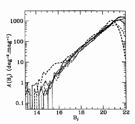
Figure 14: Determinations of the GNC in various sky regions (from Bertin & Dennefeld, 1996). The bright end wildly fluctuates around the predicted value, while at fainter magnitudes the behavior is quite smooth and is the same for the different fields.

The fact that at faint magnitudes the behavior is quite regular, is due to the smoothing of spatial fluctuations for the luminosity effect. Namely at a given apparent magnitude there are contribution from galaxies located at very different distance, as the luminosity function of galaxies is spread over several decades of luminosities. On the other hand at the bright end there are contributions only from nearby galaxies, and is such a way the space finite size fluctuations are not smoothed out.

In the data shown in Fig.8 K-corrections have been not applied. Such corrections must be present because of the Hubble distance-redshift relation. Namely the spectrum of a certain galaxy at redshift $z$ is shifted towards red of a certain amount, according to the Hubble law. There are several galaxies (E/S0) with steep spectra and hence for these one detects a lower value of the intensity of the ”true” one because of the shift of the maximum of the spectrum. However there are several other galaxies (Sdm, Scd) with flat spectra. In some case the shift due to the Hubble law may produce an higher intensity while in other a decrease of the apparent flux. The K-corrections are model dependent corrections: the sign can be in both directions, i.e. towards an increasing or a decreasing of the absolute magnitude $\!{}^{{\bf?}}$. Moreover the effect of such corrections is in general not so important for the distortion of the number counts relation $\!{}^{{\bf?}}$.

In observational astrophysics there are a lot of data which are only angular ones, as the measurements of distances is general a very complex task. We briefly discuss here the distribution of radiogalaxies, Quasars and the $\gamma$-ray burst distribution. Our conclusion is that all these data are compatible with a fractal structure with $D\approx 1.6\div 2.0$ similar to that of galaxies.

4.6 Radio galaxies

As an example of counts of objects, we consider the case of radio galaxies. The majority of catalog radio sources are extragalactic and some of the strongest are at cosmological distances. One of the most important information on radio galaxies distribution has been obtained from the sources counts as a function of the apparent flux $\!{}^{{\bf?}}$. Extensive surveys of sources have been made at various frequencies in the range $0.4\div 5\;GHz$. In Fig.15

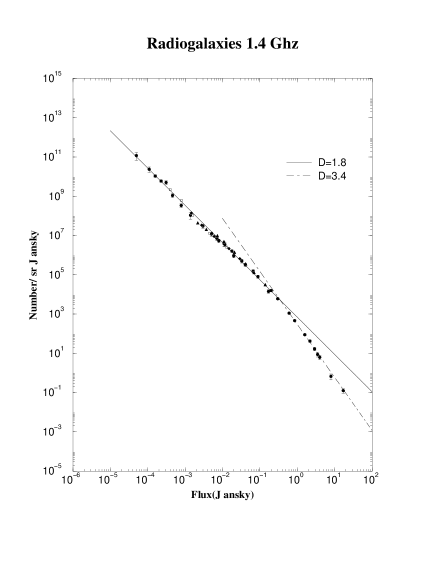
Figure 15: Normalized differential sources counts at $\nu=1.4Ghz$. Abscissa log flux density (Jy). Ordinate log differential number of sources $n(S)$. The solid line represents the behavior of a fractal structure with $D=1.8$. The amplitude has been computed from the knowledge of the luminosity function (see text). The agreement is excellent, except in the bright fluxes region due to the presence of finite size fluctuations. (From Condon, 1984).

we show a compendium of sources counts at $\nu=1.4Ghz$ $\!{}^{{\bf?}}$. The differential counts are plotted against the apparent flux. In the bright flux region there is a deviation from a power law function, while for four decades the agreement with a fractal distribution with $D\approx 1.8$ is excellent. Such a behavior has been usually explained in literature as an effect of sources/space-time evolution. Here we propose that the radio galaxies are fractally distributed, as galaxies, with almost the same fractal dimension. The deviation at bright fluxes in this picture is explained as a spurious effect due to the small scale fluctuations, as in the case of galaxy counts. In the other frequency bands the situation is nearly the same $\!{}^{{\bf?}}$. The simple picture of a fractal distribution of radio sources is therefore fully compatible with the experimental situation.

It is simple to show that the differential number of radio galaxies for unit flux (in Jansky) and unit steradian, in an Euclidean space, is given by:

$$n(S)=\frac{1}{(3\cdot 10^{9})^{2}}\left(\frac{1}{4\pi}\right)^{\frac{D+2}{2}}\frac{DB_{R}}{2}S^{-\frac{D+2}{2}}\int\phi(L)dL$$ (62)

where we have taken, as usual, $n(r)=(B_{R}D/4\pi)r^{D-3}$ and $S=L/(4\pi r^{2})$ ($L$ is the intrinsic luminosity). From the knowledge of the parameters of the luminosity function $\!{}^{{\bf?}}$ we have that a good approximation of the data reported in Fig.15 is given by $D=1.8$ and $B_{R}=0.1Mpc^{-D}$. Such a low value for $B_{R}$ implies that the density of radio galaxies is about 100 lower than that of optical galaxies. When it will be possible to have a complete redshift sample of Radio galaxies, i.e. a well defined volume limited sample, one will be able to measure directly $B_{R}$ and $D$ from the knowledge of the conditional density and hence to compare those values with the ones we have measured from the number flux relation.

4.7 Compendium of counts

In Tab.2 we summarize the behavior of the number counts for various astrophysical objects. The small scale exponent corresponds to the bright end of the number counts relation, while the large scale exponent to the faint end. The ”small scale exponent” is not a real exponent and wildly fluctuates for the different objects. On the contrary the large scale exponent is a real exponent and its value is in the range $1.8\mathrel{\hbox to0.0pt{\lower 3.0pt\hbox{$\mathchar 536\relax$}\hss}\raise 2.0pt\hbox{$\mathchar 316\relax$}}D\mathrel{\hbox to0.0pt{\lower 3.0pt\hbox{$\mathchar 536\relax$}\hss}\raise 2.0pt\hbox{$\mathchar 316\relax$}}2.2$ for almost all the cases. The counts of all these different objects is therefore compatible with a fractal distribution in space.

This implies a completely new interpretation of the counts. At small scale the exponent $D\approx 3$ (i.e $\alpha\approx 0.6$ in the case of magnitude counts) is due to finite size effects and not to a real homogeneity: this has be shown to be the case with very specific tests. On the other hand, at larger scale the value $D\approx 2$ (i.e. $\alpha\approx 0.4$) corresponds to the correct correlation properties of the samples, that we can find by the complete correlation analysis in the three dimensional space. This implies that galaxy evolution, modifications of the Euclidean Geometry and the K-corrections are not very relevant in the range of the present data. In addition the fact that the exponent $\alpha\approx 0.4$ holds up to magnitude $27\div 28$ for galaxies seems to indicate that the fractal may continue up to distances $\sim 4000h^{-1}Mpc$. Quite a remarkable fact if one considers that the Hubble radius of the Universe is supposed to be $4000h^{-1}Mpc$. Moreover such a behavior can be found for galaxies in the different photometric bands, as well as for other astrophysical objects.

Objects	Small scale behavior		Large scale behavior
U-band1	$?\mathrel{\hbox to0.0pt{\lower 3.0pt\hbox{$\mathchar 536\relax$}\hss}\raise 2.0pt\hbox{$\mathchar 316\relax$}}U\mathrel{\hbox to0.0pt{\lower 3.0pt\hbox{$\mathchar 536\relax$}\hss}\raise 2.0pt\hbox{$\mathchar 316\relax$}}18$	$D\approx?$	$18\mathrel{\hbox to0.0pt{\lower 3.0pt\hbox{$\mathchar 536\relax$}\hss}\raise 2.0pt\hbox{$\mathchar 316\relax$}}U\mathrel{\hbox to0.0pt{\lower 3.0pt\hbox{$\mathchar 536\relax$}\hss}\raise 2.0pt\hbox{$\mathchar 316\relax$}}24$	$D\approx 2.5$
B-band2	$12\mathrel{\hbox to0.0pt{\lower 3.0pt\hbox{$\mathchar 536\relax$}\hss}\raise 2.0pt\hbox{$\mathchar 316\relax$}}B\mathrel{\hbox to0.0pt{\lower 3.0pt\hbox{$\mathchar 536\relax$}\hss}\raise 2.0pt\hbox{$\mathchar 316\relax$}}18$	$D\approx 3$	$18\mathrel{\hbox to0.0pt{\lower 3.0pt\hbox{$\mathchar 536\relax$}\hss}\raise 2.0pt\hbox{$\mathchar 316\relax$}}B\mathrel{\hbox to0.0pt{\lower 3.0pt\hbox{$\mathchar 536\relax$}\hss}\raise 2.0pt\hbox{$\mathchar 316\relax$}}28$	$D\approx 2$
V-band3	$\mathrel{\hbox to0.0pt{\lower 3.0pt\hbox{$\mathchar 536\relax$}\hss}\raise 2.0pt\hbox{$\mathchar 316\relax$}}20$	$D\approx?$	$22\mathrel{\hbox to0.0pt{\lower 3.0pt\hbox{$\mathchar 536\relax$}\hss}\raise 2.0pt\hbox{$\mathchar 316\relax$}}V\mathrel{\hbox to0.0pt{\lower 3.0pt\hbox{$\mathchar 536\relax$}\hss}\raise 2.0pt\hbox{$\mathchar 316\relax$}}25$	$D\approx 1.95$
R-band4	$15\mathrel{\hbox to0.0pt{\lower 3.0pt\hbox{$\mathchar 536\relax$}\hss}\raise 2.0pt\hbox{$\mathchar 316\relax$}}R\mathrel{\hbox to0.0pt{\lower 3.0pt\hbox{$\mathchar 536\relax$}\hss}\raise 2.0pt\hbox{$\mathchar 316\relax$}}18$	$D\approx 2.8$	$20\mathrel{\hbox to0.0pt{\lower 3.0pt\hbox{$\mathchar 536\relax$}\hss}\raise 2.0pt\hbox{$\mathchar 316\relax$}}R\mathrel{\hbox to0.0pt{\lower 3.0pt\hbox{$\mathchar 536\relax$}\hss}\raise 2.0pt\hbox{$\mathchar 316\relax$}}26$	$D\approx 1.85$
I-band5	$?\mathrel{\hbox to0.0pt{\lower 3.0pt\hbox{$\mathchar 536\relax$}\hss}\raise 2.0pt\hbox{$\mathchar 316\relax$}}I\mathrel{\hbox to0.0pt{\lower 3.0pt\hbox{$\mathchar 536\relax$}\hss}\raise 2.0pt\hbox{$\mathchar 316\relax$}}19$	$D\approx?$	$19\mathrel{\hbox to0.0pt{\lower 3.0pt\hbox{$\mathchar 536\relax$}\hss}\raise 2.0pt\hbox{$\mathchar 316\relax$}}I\mathrel{\hbox to0.0pt{\lower 3.0pt\hbox{$\mathchar 536\relax$}\hss}\raise 2.0pt\hbox{$\mathchar 316\relax$}}25$	$D\approx 1.7$
K-band6	$12\mathrel{\hbox to0.0pt{\lower 3.0pt\hbox{$\mathchar 536\relax$}\hss}\raise 2.0pt\hbox{$\mathchar 316\relax$}}K\mathrel{\hbox to0.0pt{\lower 3.0pt\hbox{$\mathchar 536\relax$}\hss}\raise 2.0pt\hbox{$\mathchar 316\relax$}}17$	$D\approx 3.35$	$20\mathrel{\hbox to0.0pt{\lower 3.0pt\hbox{$\mathchar 536\relax$}\hss}\raise 2.0pt\hbox{$\mathchar 316\relax$}}K\mathrel{\hbox to0.0pt{\lower 3.0pt\hbox{$\mathchar 536\relax$}\hss}\raise 2.0pt\hbox{$\mathchar 316\relax$}}24$	$D\approx 1.6$
Quasars7	$14.75\mathrel{\hbox to0.0pt{\lower 3.0pt\hbox{$\mathchar 536\relax$}\hss}\raise 2.0pt\hbox{$\mathchar 316\relax$}}B\mathrel{\hbox to0.0pt{\lower 3.0pt\hbox{$\mathchar 536\relax$}\hss}\raise 2.0pt\hbox{$\mathchar 316\relax$}}18.75$	$D\approx 4.4$	$19\mathrel{\hbox to0.0pt{\lower 3.0pt\hbox{$\mathchar 536\relax$}\hss}\raise 2.0pt\hbox{$\mathchar 316\relax$}}B\mathrel{\hbox to0.0pt{\lower 3.0pt\hbox{$\mathchar 536\relax$}\hss}\raise 2.0pt\hbox{$\mathchar 316\relax$}}23$	$D\approx 1.5$
Radio8 $\nu=1.4Ghz$	$1\mathrel{\hbox to0.0pt{\lower 3.0pt\hbox{$\mathchar 536\relax$}\hss}\raise 2.0pt\hbox{$\mathchar 316\relax$}}S\mathrel{\hbox to0.0pt{\lower 3.0pt\hbox{$\mathchar 536\relax$}\hss}\raise 2.0pt\hbox{$\mathchar 316\relax$}}10$	$D\approx 3.44$	$10^{-5}\mathrel{\hbox to0.0pt{\lower 3.0pt\hbox{$\mathchar 536\relax$}\hss}\raise 2.0pt\hbox{$\mathchar 316\relax$}}S\mathrel{\hbox to0.0pt{\lower 3.0pt\hbox{$\mathchar 536\relax$}\hss}\raise 2.0pt\hbox{$\mathchar 316\relax$}}1$	$D\approx 1.8$
Radio8 $\nu=0.61Ghz$	$1\mathrel{\hbox to0.0pt{\lower 3.0pt\hbox{$\mathchar 536\relax$}\hss}\raise 2.0pt\hbox{$\mathchar 316\relax$}}S\mathrel{\hbox to0.0pt{\lower 3.0pt\hbox{$\mathchar 536\relax$}\hss}\raise 2.0pt\hbox{$\mathchar 316\relax$}}10$	$D\approx 3.8$	$10^{-3}\mathrel{\hbox to0.0pt{\lower 3.0pt\hbox{$\mathchar 536\relax$}\hss}\raise 2.0pt\hbox{$\mathchar 316\relax$}}S\mathrel{\hbox to0.0pt{\lower 3.0pt\hbox{$\mathchar 536\relax$}\hss}\raise 2.0pt\hbox{$\mathchar 316\relax$}}1$	$D\approx 1.6$
Radio8 $\nu=0.408Ghz$	$1\mathrel{\hbox to0.0pt{\lower 3.0pt\hbox{$\mathchar 536\relax$}\hss}\raise 2.0pt\hbox{$\mathchar 316\relax$}}S\mathrel{\hbox to0.0pt{\lower 3.0pt\hbox{$\mathchar 536\relax$}\hss}\raise 2.0pt\hbox{$\mathchar 316\relax$}}10$	$D\approx 3.7$	$10^{-3}\mathrel{\hbox to0.0pt{\lower 3.0pt\hbox{$\mathchar 536\relax$}\hss}\raise 2.0pt\hbox{$\mathchar 316\relax$}}S\mathrel{\hbox to0.0pt{\lower 3.0pt\hbox{$\mathchar 536\relax$}\hss}\raise 2.0pt\hbox{$\mathchar 316\relax$}}1$	$D\approx 1.5$
Radio8 $\nu=5.0Ghz$	$1\mathrel{\hbox to0.0pt{\lower 3.0pt\hbox{$\mathchar 536\relax$}\hss}\raise 2.0pt\hbox{$\mathchar 316\relax$}}S\mathrel{\hbox to0.0pt{\lower 3.0pt\hbox{$\mathchar 536\relax$}\hss}\raise 2.0pt\hbox{$\mathchar 316\relax$}}10$	$D\approx 3.4$	$10^{-4}\mathrel{\hbox to0.0pt{\lower 3.0pt\hbox{$\mathchar 536\relax$}\hss}\raise 2.0pt\hbox{$\mathchar 316\relax$}}S\mathrel{\hbox to0.0pt{\lower 3.0pt\hbox{$\mathchar 536\relax$}\hss}\raise 2.0pt\hbox{$\mathchar 316\relax$}}1$	$D\approx 1.8$
X-ray sources9	$5\cdot 10^{-13}\mathrel{\hbox to0.0pt{\lower 3.0pt\hbox{$\mathchar 536\relax$}\hss}\raise 2.0pt\hbox{$\mathchar 316\relax$}}S\mathrel{\hbox to0.0pt{\lower 3.0pt\hbox{$\mathchar 536\relax$}\hss}\raise 2.0pt\hbox{$\mathchar 316\relax$}}10^{-12}$	$D\approx 3.4$	$10^{-16}\mathrel{\hbox to0.0pt{\lower 3.0pt\hbox{$\mathchar 536\relax$}\hss}\raise 2.0pt\hbox{$\mathchar 316\relax$}}S\mathrel{\hbox to0.0pt{\lower 3.0pt\hbox{$\mathchar 536\relax$}\hss}\raise 2.0pt\hbox{$\mathchar 316\relax$}}5\cdot 10^{-13}$	$D\approx 1.8$
$\gamma-ray$ bursts 10	$10\mathrel{\hbox to0.0pt{\lower 3.0pt\hbox{$\mathchar 536\relax$}\hss}\raise 2.0pt\hbox{$\mathchar 316\relax$}}S\mathrel{\hbox to0.0pt{\lower 3.0pt\hbox{$\mathchar 536\relax$}\hss}\raise 2.0pt\hbox{$\mathchar 316\relax$}}100$	$D\approx 3$	$10^{-1}\mathrel{\hbox to0.0pt{\lower 3.0pt\hbox{$\mathchar 536\relax$}\hss}\raise 2.0pt\hbox{$\mathchar 316\relax$}}S\mathrel{\hbox to0.0pt{\lower 3.0pt\hbox{$\mathchar 536\relax$}\hss}\raise 2.0pt\hbox{$\mathchar 316\relax$}}10$	$D\approx 1.7$

Table 2: The exponents of counts for different kinds of astrophysical objects (see text). (Ref.1-6: see Table 8; Ref.7: Hartwick & Schade, 1990; Ref.8: Condon,1984; Ref.9: Hasinger et al., 1993; Ref.10: Meegan et al.1995)

5 Conclusion

The highly irregular galaxy distributions with large structures and voids strongly point to a new statistical approach in which the existence of a well defined average density is not assumed a priori and the possibility of non analytical properties should be addressed specifically. The new approach for the study of galaxy correlations in all the available catalogues shows that their properties are actually compatible with each other and they are statistically valid samples. The severe discrepancies between different catalogues that have led various authors to consider these catalogues as not fair, were due to the inappropriate methods of analysis.

The correct two point correlation analysis shows well defined fractal correlations up to the present observational limits, from 1 to $1000h^{-1}Mpc$ with fractal dimension $D\simeq 2$. Of course the statistical quality and solidity of the results is stronger up to $100\div 200h^{-1}Mpc$ and weaker for larger scales due to the limited data. It is remarkable, however, that at these larger scales one observes exactly the continuation of the correlation properties of the small and intermediate scales.

From the theoretical point of view the fact that we have a situation characterized by self-similar structures implies that we should not use concept like $\xi(r)$, $r_{0}$, $\delta N/N$ and certain properties of the power spectrum, because they are not suitable to represent the real properties of the observed structures. In this respect also the N-body simulations should be considered from a new perspective. One cannot talk about ”small” or ”large” amplitudes for a self-similar structure because of the lack of a reference value like the average density. The Physics should shift from ”amplitudes” towards ”exponent” and the methods of modern statistical Physics should be adopted. This requires the development of constructive interactions between two fields.

References

References

- [1] Coleman, P.H. & Pietronero, L., Phys.Rep. 231, (1992) 311
- [2] Baryshev, Y., Sylos Labini, F., Montuori, M., Pietronero, L. Vistas in Astron. 38, (1994) 419
- [3] Pietronero, L., Montuori, M. and Sylos Labini, F., in the Proc of the Conference ”Critical Dialogues in Cosmology” N. Turok Ed. (1997) World Scientific
- [4] Sylos Labini, F., Montuori, M., Pietronero, L. phys.Rep. 291, (1997) In print
- [5] Davis, M., in the Proc of the Conference ”Critical Dialogues in Cosmology” N. Turok Ed. (1997) World Scientific
- [6] Davis, M., Peebles, P. J. E. Astrophys. J., 267, (1983) 465
- [7] Sylos Labini F. & Pietronero L., Astrophys.J., (1996), 469, 28
- [8] Schecther, P., Astrophys.J. 203, (1976) 297
- [9] Da Costa, L. N. et al. Astrophys. J. 424, (1994) L1
- [10] Vettolani, G., et al. (1994) Proc. of Scloss Rindberg workshop Studying the Universe with Clusters of Galaxies
- [11] Mandelbrot B., (1982) The Fractal Geometry of Nature, Freeman, New York
- [12] Sylos Labini F., Astrophys. J., 433, (1994) 464
- [13] Peebles P. J. E., (1993) Principles of physical cosmology, Princeton Univ. Press
- [14] Paturel g., Vauglin I., Garnier R., Marthinet M.C., Petit C., Di Nella H., Bottinelli L., Gouguenheim L., Durand N., in ”Databases and On-Line data in astronomy” Eds. Egert D. and Albrecht M., (1995) Knluwer Academic Publisher
- [15] Schectman S. et al., Astrophys. J., (1996) 470,172
- [16] Saunders W., Rowan Robinson M., Lawrence A., Efstathiou G., Kaiser N., Ellis R.S. and Frenk C.S. Mon.Not.R.Astr.Soc. 242, (1990) 318
- [17] Sylos Labini F., Gabrielli A., Montuori M., Pietronero L., Physica A, 226, (1996) 195
- [18] Voronoi, J. Reine Angew. Math. 134, (1908) 198
- [19] Badii R., and Politi A. Physics Letters A (1984) 104, 303
- [20] Smith L.A., Fournier J.-D. and Spiegel E.A., Physics Letters A (1986) 114, 465
- [21] Sornette D., Johansen A., Arneodo A., Muzy J.F. and Saleur H., Phys. Rev. Letters (1996) 76, 251
- [22] Solis F.J. and Tao L., (1997) preprint (cond-mat/9703051)
- [23] Broadhurst, T. J., et al.Nature, 343, (1990) 726
- [24] Willmer C.N.A. et al.Astrophys.J., 437, (1994) 560
- [25] Ettori S., Guzzo L. and Tarenghi M. Mon.Not.R.Astr.Soc. (1996), in press
- [26] Cohen J.G. et al., (1996) in prints (astro-ph/9608121)
- [27] Bellanger C. & De Lapparent V. Astrophys.J., 455, (1995) L1
- [28] Hubble, E. Astrophys.J. 64, (1926) 321
- [29] Metcalfe, N., Shanks, T., Fong, R., Jones L.R., Mon.Not.R.Astr.Soc. 249, (1991) 498 Nature, 367, (1994) 538.
- [30] Tyson, J.A., Astron.J. , 96, (1988) 1
- [31] Lilly, S. J., Cowie, L. L. and Gardner, J. P., Astrophys.J. . 369, (1991) 79
- [32] Jones L. R., Fong, R., Shanks, T., Ellis, R. S., & Peterson, B. A., Mon.Not.R.Astr.Soc. , 249, (1991) 481
- [33] Driver S.P., Phillipps S., Davies J.I., Morgan I. and Disney M.J. Mon.Not.R.Astr.Soc. 266, (1994) 155
- [34] Yoshii, & Peterson, Astrophys.J,. 444, (1995)15
- [35] Yoshii, Yu., Takahara, F. Astrophys. J. 326, (1988)1
- [36] Cowie L., Gardner, J. P., Lilly S. J., McLean, I. Astrophys.J. 360, (1990) L1
- [37] Cowie, (1991) in Observational test of Cosmological Inflation, ed. T. Shanks, A. J. Bandy, R. S. Ellis, C. S. Frenk, & A. W. Wolfendale (Dordrecht: Kluwer), 257
- [38] Yoshii, Astrophys.J, 403, (1993) 552
- [39] Broadhurst, T. J., Ellis, R., S. & Glazebrook, K. Nature, 355, (1992) 55
- [40] Haynes, M., Giovanelli, R., (1988) in ”Large-scale motion in the Universe”, Eds. Rubin, V.C., Coyne, G., Princeton University Press, Princeton L133
- [41] Bertin E. and Dennefeld M., Astron.Astrophys., 317, (1996) 413
- [42] Pence W. Astrophys.J., 203, (1976) 39
- [43] Condon J. J. Astrophys.J., 287, (1984) 461