On the nature of SW Sex

Abstract

We present spectrophotometry of the eclipsing nova-like variable SW Sex. The continuum is deeply eclipsed and shows asymmetries due to the presence of a bright spot. We derive a new ephemeris and, by measuring the eclipse width, we are able to constrain the inclination to $i>75^{\circ}$ and the disc radius to $R_{D}>0.6L_{1}$. In common with other members of its class (of which it is the proto-type), SW Sex shows single-peaked emission lines which show transient absorption features and large phase shifts in their radial velocity curves. In addition, the light curves of the emission lines show a reduction in flux around phase 0.5 and asymmetric eclipse profiles which are not as deep as the continuum eclipse. Using Doppler tomography, we find that most of the line emission in SW Sex appears to originate from three sources: the secondary star, the accretion disc and an extended bright spot. The detection of the red star allows us to constrain the radial-velocity semi-amplitude of the secondary to $K_{R}>180$ km s^-1 and hence the component masses to $M_{1}\sim 0.3-0.7M_{\odot}$ and $M_{2}<0.3M_{\odot}$.

The Doppler maps suggest a simple new model for SW Sex in which the dominance of single-peaked line emission from the bright spot over the weak double-peaked disc emission gives SW Sex its single-peaked profiles and forces the radial-velocity curves to follow the motion of the bright spot and thus exhibit large phase shifts. The transient absorption features in the Balmer-line profiles are mostly artifacts of the complex intertwining of the emission components from the secondary star, bright spot and accretion disc and involve little true absorption. While the accretion disc and secondary star components of this model appear to be secure, the dominant bright-spot component fails in one important area – its inconsistency with the Balmer-line light curves. The eclipse profile requires the material emitting the Balmer lines to be eclipsed as early as phase 0.8, but which is not as deeply eclipsed as the continuum, exhibits a flat bottomed eclipse and then comes out of eclipse very sharply around phase 0.05. Although it is possible to explain the early ingress with a raised disc rim downstream from the bright-spot, the rapid egress is difficult to account for without speculating that either there are regions of strong Balmer absorption in the disc whose changing visibility during eclipse alters the shape of the light curve or that there is Balmer emission from above the orbital plane which shares the velocity of the bright-spot.

1 Introduction

Cataclysmic variables (CVs) are close binary stars consisting of a red dwarf secondary transferring material on to a white dwarf primary via an accretion disc or magnetic accretion stream. Nova-like variables are defined as CVs which have never been observed to undergo nova or dwarf-nova type outbursts (see warner95 and dhillon96 for reviews). This is due to the fact that nova-likes are believed to harbour steady-state accretion discs, one of the foundations of accretion disc theory [Pringle1981]. Recent advances in accretion disc research have been based on studying nova-like variables (e.g. rutten93), but it has become increasingly clear that there may be problems with this approach due to the SW Sex phenomenon, which throws into question even the very existence of accretion discs in these systems [Williams1989].

The SW Sex phenomenon, a term first coined by thorstensen91a, is peculiar to a group of high-inclination nova-like variables with periods in the range 3–4 hr. All of these so-called SW Sex stars exhibit strong, single-peaked Balmer, He I and He II emission lines which, with the exception of He II, remain largely unobscured during primary eclipse. This is in stark contrast to standard accretion disc theory, which predicts that emission lines from high-inclination discs should appear double-peaked and be eclipsed once every orbital period (e.g. horne86). In addition, the emission lines in SW Sex stars show strong phase-dependent absorption features and their radial velocity curves exhibit significant phase shifts relative to photometric minimum. Three competing models claim to satisfy these observational constraints, with varying degrees of success: an accretion disc wind [Honeycutt, Schlegel & Kaitchuck1986], magnetic accretion [Williams1989] or a bright-spot overflow (hellier94).

With the intent of discriminating between these opposing models, we obtained spectrophotometry of the proto-type of the class, SW Sex. This object (also known as PG 1012–029) was one of 22 CVs discovered by their UV excesses in photographic films obtained for the Palomar-Green survey [Green, Schmidt & Liebert1986]. Follow-up spectroscopic observations of this $V\sim 14.8$ mag object by green82 revealed a high-excitation emission-line spectrum, suggesting a nova-like variable classification. The first extensive photometric and spectroscopic study of SW Sex was presented by penning84, who discovered 1.9 mag eclipses recurring on a 3.24 hr orbital period. This work was followed by the higher-resolution spectroscopic studies of Honeycutt et al. (1986; see also kaitchuck94) and williams89, who reached different conclusions as to the nature of these systems, the former invoking an accretion disc wind and the latter a magnetic accretion stream to explain the single-peaked, uneclipsed emission line profiles. The phase dependent absorption features observed by honeycutt86 were studied in greater detail by szkody90, but they were unable to account for the behaviour with a simple model. High-speed photometry by rutten92b revealed a prominent bright spot in SW Sex (also seen by ashoka94) and the resulting eclipse maps showed a flatter run of effective temperature with radial distance from disc centre than that predicted by steady-state disc theory. Despite the more recent efforts of still95, who presented a high signal-to-noise but relatively low spectral-resolution study of SW Sex, no real progress has been made in unravelling the SW Sex phenomenon, a situation which we hope to redress in the present paper.

2 Observations

We obtained a total of 83 spectra of SW Sex on the night of 1990 January 18 (orbital phases 26456.5686–26457.6282) and 75 spectra on 1990 January 19 (orbital phases 26464.0394–26464.9781) with the 2.5-m Isaac Newton Telescope (INT) on La Palma. The exposures were all 120-s long with about 9-s dead-time for the archiving of data. The Intermediate Dispersion Spectrograph (IDS) coupled with the Image Photon Counting System (IPCS, camera format 2048$\times$130 pixel) and a grating of 1200 line mm^-1 gave a wavelength coverage of approximately 4025–5050 Å at 1.1 Å ($\simeq$75 km s^-1) resolution. Comparison arc spectra were taken every $\sim$40 min to calibrate the wavelength scale and instrumental flexure. We were able to correct for slit losses by placing a nearby comparison star on the 140$\times$1.1 arcsec² slit and obtaining a photometric spectrum through a wide (5.3 arcsec) slit. We also took a spectrum of the standard star PG 0823+546 [Massey et al.1988] to correct the large-scale instrumental response and place the data on an absolute flux scale.

3 Data Reduction

The first step in the data reduction was the division of each frame by a normalized tungsten-lamp flat-field, which we used to correct for medium-scale sensitivity variations of the detector; the large-scale variations were removed using the standard star, while the small-scale variations were removed by the IPCS scanning coils [Jorden & Fordham1986]. The sky was removed by subtracting third-order polynomial fits to sky regions on either side of the SW Sex spectra. Extracted spectra were then obtained by summing across the stellar profile. The same procedure was applied to the comparison star spectra. The wavelength scale for each spectrum was interpolated from the wavelength scales of two neighbouring arc spectra, extracted from the same location on the detector as the object. The rms scatter of the sixth-order polynomial fits to the arc lines was always $<$0.1 Å. We applied a standard correction for extinction. Our final procedure was to correct for large-scale instrumental sensitivity variations and slit losses in order to obtain absolute fluxes. Each spectrum was first divided by a spline fit to the ratio of the observed count rate to the tabulated flux of PG 0823+546. The comparison star was too faint to allow for a wavelength-dependent slit-loss correction, so each SW Sex spectrum was then divided by the total flux in the corresponding comparison star spectrum and multiplied by the total flux in the wide slit comparison star spectrum.

4 Results

4.1 Ephemeris

Table 1: Eclipse observations of SW Sex. The differences between the observed and calculated times of mid-eclipse are given by O–C. The first 6 eclipse timings have been reproduced from penning84 and the last 6 from ashoka94. The remaining 9 eclipse timings have been kindly provided by René Rutten (private communication).

HJD (mid-eclipse)	Cycle Number	O–C
(2 440 000+)	($E$)	(s)
4339.65087	0	4.3
4340.73055	8	19.2
4348.82649	68	–12.4
4631.92758	2166	11.7
4676.86195	2499	0.9
4721.79636	2832	–6.4
7566.56813	23914	–11.8
7615.41619	24276	18.6
7615.55065	24277	–22.8
7616.49516	24284	–27.9
7618.51922	24299	–29.3
7619.46374	24306	–33.5
7620.40856	24313	–11.8
7621.48834	24321	11.7
7622.43257	24328	–17.6
7921.32167	26543	25.1
7921.45633	26544	1.0
7950.19842	26757	18.8
7950.33321	26758	6.0
8306.30100	29396	25.9
8306.43599	29397	30.3

We derived an ephemeris for SW Sex by adding the 9 times of mid-eclipse observed by René Rutten (private communication; see Table 1) to the 6 eclipse timings of penning84 and the 6 of ashoka94. A linear least-squares fit to these data yields the following ephemeris:

$\begin{array}[]{rrrl}T_{\rm mid-eclipse}=&\!\!\!\!\!{\em HJD}\,\,2\,444\,339.650821&\!\!+\,\,0.1349384229&\!\!\!\!\!E\\ &\!\!\pm\,\,0.000043&\!\!\pm\,\,0.0000000020&\\ \end{array}$

The errors in the ephemeris have been derived using uncertainties of 0.0001 days in the times of mid-eclipse. Only the times of mid-eclipse provided by René Rutten actually had published uncertainty values. We justify the use of the same errors for the data of penning84 and ashoka94 because the former quoted times of mid-eclipse to 4 decimal places (implying the error is in the last digit) and the data of ashoka94 are qualitatively similar to the other two datasets (implying the error must be similar). Note that we did not include our two spectrophotometrically-measured eclipse timings as the uncertainties on these points are much greater than the photometrically-measured points given in Table 1 (due to the poorer time resolution) and our points were also observed very close in time to those of ashoka94.

The differences between the observed and calculated times of mid-eclipse (O–C) are given in Table 1. Given that most of the points cluster around two widely-separated epochs and that the typical O–C values derived from the linear ephemeris are of the same order as the uncertainties in the mid-eclipse timings, we do not think a search for variations in the orbital period (e.g. by fitting a parabola, see pringle75) is justified.

4.2 Inclination and disc radius

Figure 1: Upper panel – orbital inclination as a function of mass ratio for three different values of the eclipse width, $\Delta\phi_{1/2}=$ 0.095, 0.098 and 0.101. Lower panel – accretion disc radius as a function of mass ratio for three different values of the eclipse width, $\Delta\phi=$ 0.10, 0.12 and 0.14.

By considering the geometry of a point eclipse by a spherical body, it is possible to determine the inclination, $i$, of a binary system through the relation

$$\left(\frac{R_{2}}{a}\right)^{2}=\sin^{2}(\pi\Delta\phi_{1/2})+\cos^{2}(\pi\Delta\phi_{1/2})\cos^{2}{i},$$ (1)

where $R_{2}/a$ is defined as the volume radius of the secondary star and can be expressed solely as a function of the mass ratio, $q=M_{2}/M_{1}$ [Eggleton1983]:

$$\frac{R_{2}}{a}=\frac{0.49q^{2/3}}{0.6q^{2/3}+\ln(1+q^{1/3})}.$$ (2)

$\Delta\phi_{1/2}$ is the mean phase full-width of eclipse at half the out-of-eclipse intensity, which from the sum of the quasi-$B$-band eclipses of rutten92b was measured to be $\Delta\phi_{1/2}=0.098\pm 0.003$ (René Rutten, private communication). This figure is in good agreement with the eclipse widths derived from a visual inspection of Fig. 8 of penning84 and Fig. 8 of ashoka94, which have a value of $\Delta\phi_{1/2}\sim 0.1$. The upper panel of Fig. 1 shows the $q$ versus $i$ relation for this eclipse width and its error, calculated using equations (1) and (2). These curves agree to better than 1 per cent with those obtained using an exact computation of the Roche-lobe geometry (see dhillon92). Even without a reliable estimate of the mass ratio, we can constrain the inclination of SW Sex from Fig. 1 to be $i>75^{\circ}$. Note that penning84 derived a value of $i=79^{\circ}\pm 1^{\circ}$, but this figure is based on a dubious radial velocity analysis (see section 4.9).

The quasi-$B$-band continuum eclipses of rutten92b have a mean phase half-width at maximum light (ie. timing the first and last contacts of eclipse and dividing by 2) of $\Delta\phi=0.12\pm 0.02$ (René Rutten, private communication). Following the method of sulkanen81, it is possible to determine the radius of the accretion disc, $R_{D}$, in SW Sex through the geometric relation

$$R_{D}=a\sin{i}\sin{(2\pi\Delta\phi)}-R_{C},$$ (3)

where the half-chord on the secondary, $R_{C}$, is known in terms of $i$ and $R_{2}/a$:

$$\frac{R_{C}}{a}=\sqrt{\left(\frac{R_{2}}{a}\right)^{2}-\cos^{2}{i}}.$$ (4)

The lower panel of Fig. 1 shows a plot of the disc radius versus mass ratio for three values of the eclipse width, $\Delta\phi=0.12\pm 0.02$. The curves were produced by determining the inclination for each mass ratio using equations (1) and (2), assuming $\Delta\phi_{1/2}=0.098$, and then calculating the disc radius for this inclination and mass ratio using equations (3) and (4). These curves agree to better than 5 per cent with those obtained using an exact computation of the Roche-lobe geometry (see dhillon91). The dashed curve represents solutions where $R_{D}<R_{C}$, i.e. solutions where we would expect to see a total (flat-bottomed) eclipse. This is clearly not the case for SW Sex, which exhibits round-bottomed eclipses (e.g. rutten92b). The accretion disc in SW Sex must therefore have a radius which lies between 0.6$L_{1}$ (where $L_{1}$ is the distance between the white dwarf and the inner Lagrangian point) and the radius of the primary Roche lobe, implying that the disc in SW Sex is comparable in size to the discs of other nova-like variables and dwarf novae in outburst, but is larger than the discs of dwarf novae in quiescence (see harrop96).

4.3 Average spectrum

Figure 2: The average of all 158 spectra of SW Sex, uncorrected for orbital motion.

Table 2: Fluxes, equivalent widths and velocity widths of prominent lines in the average spectrum of SW Sex (Fig. 2). The errors on the flux, EW, FWHM and FWZI measurements are of order 0.1 erg cm^-2 s^-1, 1 Å, 100 km s^-1 and 1000 km s^-1, respectively.

Line	Flux	EW	FWHM	FWZI
	$\times$10-13	Å	km s-1	km s-1
	erg cm -2 s-1
H$\beta$	1.22	17.3	1270	4500
H$\gamma$	1.09	13.3	1290	4800
H$\delta$	1.12	13.6	1450	4500
HeI $\lambda$4471	0.27	3.3	1500	3000
HeI $\lambda$4921	0.21	3.1
HeI $\lambda$5015	0.09	1.4
HeII $\lambda$4542	0.06	0.8
HeII $\lambda$4686	1.15	15.2	1400	5700
CII $\lambda$4267	0.24	2.9	1600	4500
CIII/NIII	0.77	9.9	1500	5000

Figure 3: Orbital emission line variations in SW Sex. The data have been averaged into 10 binary phase bins, with a multiple of 4 added to each spectrum in order to displace the data in the vertical direction.

The average of all 158 spectra of SW Sex, uncorrected for orbital motion, is displayed in Fig. 2. A direct comparison of this spectrum with that of a number of other SW Sex stars is given in Fig. 5 of dhillon96. In common with most other high-inclination nova-like variables, including magnetic systems (e.g. FO Aqr; marsh96), SW Sex shows a number of features very different from those exhibited by high-inclination dwarf novae (e.g. IP Peg; marsh88a). The low-excitation Balmer and He I lines show symmetric, single-peaked profiles instead of the double-peaked profiles one would expect from a high-inclination accretion disc. The high-excitation lines of He II $\lambda$4686 Å, He II $\lambda$4542 Å, C II $\lambda$4267 Å and C III/N III $\lambda$4640–4650 Å are very strong, much more prominent than in most quiescent dwarf novae, and also exhibit symmetric, single-peaked profiles. In addition, there appear to be many weak features in the continuum not usually seen in dwarf novae.

In Table 2 we list fluxes, equivalent widths and velocity widths of the most prominent lines in the average spectrum of SW Sex. The Balmer decrement is flat, indicating that the emission is optically thick, as is usually the case for cataclysmic variables. The FWHM of the lines are comparable to those observed in other SW Sex stars (e.g. V1315 Aql; dhillon91), but are small compared to the FWHM of emission lines in high-inclination dwarf novae (e.g. IP Peg; marsh88a). The FWZI of the emission lines in SW Sex, however, are comparable with those observed in IP Peg. This indicates that the emission lines in SW Sex (and other members of its class) have narrow cores and broad wings when compared with the profiles expected of a canonical high-inclination accretion disc. The average spectrum of SW Sex does differ slightly from the other members of its class in one respect – the ratio of the strength of the high-excitation features to the strength of the Balmer lines is larger in SW Sex than is commonly observed in other SW Sex stars.

4.4 Emission line variations

We rebinned the spectra on to a uniform wavelength scale and cast the data into 10 binary phase bins by averaging all the spectra falling into each bin. A multiple of 4 was then added to each spectrum in order to displace the data along the ordinate. The result is plotted in Fig. 3.

The Balmer line-profile variations are extremely complex and very similar to those observed in other SW Sex stars (e.g. DW UMa, shafter88; V1315 Aql, dhillon91). The lines are single peaked, but show transient absorption features at phases 0.2–0.4 and 0.6–0.9, giving the profiles a double-peaked appearance. The absorption features in SW Sex are not as deep as those in V1315 Aql and they appear to be visible for a greater fraction of the orbit. The He I lines, and to a lesser extent the C II $\lambda$4267 Å line, show absorption features which behave in a similar way to the Balmer lines. The lines of He II $\lambda$4686 Å and C III/N III $\lambda$4640–4650 Å, on the other hand, appear to be single peaked for the entire orbit. The spectrum at the foot of Fig. 3 shows that the lines are relatively unchanged by primary eclipse, in approximate agreement with the behaviour of other SW Sex stars. Note, however, that He II $\lambda$4686 Å and C III/N III $\lambda$4640–4650 Å appear to be more deeply eclipsed in V1315 Aql than in SW Sex.

Figure 4: Continuum and line light curves of SW Sex. The open circles represent points where the real data (closed circles) have been folded over.

4.5 Light curves

We binned the data into 75 phase bins and fitted the continuum of each spectrum with a third-order polynomial. The flux in each line was then derived by summing the residual flux in the line after continuum subtraction. Fig. 4 shows the continuum light curve (measured between 4490–4590 Å and 4730–4820 Å) and those of H$\beta$, H$\gamma$, H$\delta$, He I $\lambda$4471 Å, C II $\lambda$4267 Å and the sum of He II $\lambda$4686 Å and C III/N III $\lambda$4640–4650 Å. Note that the data have been folded so as to display more than one binary cycle.

A direct comparison of these light curves with those of a number of other SW Sex stars is given in Fig. 5 of dhillon96. The continuum light curve shows a deep, rounded eclipse, with a small hump before primary eclipse and a shoulder during egress. ashoka94 observed a similar hump prior to eclipse on three consecutive orbits of SW Sex, thereby ruling out the possibility that the humps are due to flickering. The origin of these features is almost certainly due to the changing aspect of the bright-spot and is supported by the appearance of the strong bright-spot, contributing 13 per cent of the total light, in the eclipse maps of SW Sex presented by rutten92b.

The Balmer-line light curves are remarkable. They are not as deeply eclipsed as the continuum and show wide, asymmetric eclipse profiles with a broad ingress and very steep egress. The ingress is particularly wide in H$\gamma$ and H$\delta$, implying that some of the line flux is eclipsed as early as phase $\sim 0.8$, which is too early to be explained in terms of obscuration by the secondary star. The eclipses in H$\gamma$ and H$\delta$ appear to reach a minimum before phase 0 and show flat-bottomed profiles. The egress in these lines is extremely rapid, commencing around phase 0.01 and completing by phase 0.05. There is also evidence for a reduction in line flux around phase 0.5 in all of the Balmer lines, as observed so prominently in other SW Sex stars, and this feature becomes stronger as one moves up the Balmer series. The He I $\lambda$4471 Å line shows a similar eclipse profile to H$\delta$, but the eclipse is deeper and the phase 0.5 absorption much stronger. The C II $\lambda$4267 Å line shows an eclipse shape which is reversed to that of the other lines, with a narrow ingress and a broad egress which finishes at phase $\sim 0.2$ (too late to be explained in terms of obscuration by the secondary star). The He II $\lambda$4686 Å and C III/N III $\lambda$4640–4650 Å light curve is the only one which comes close to resembling the continuum light curve – the eclipse is deep and approximately of the same width as the continuum eclipse, although less rounded, and appears to be preceded by a small orbital hump.

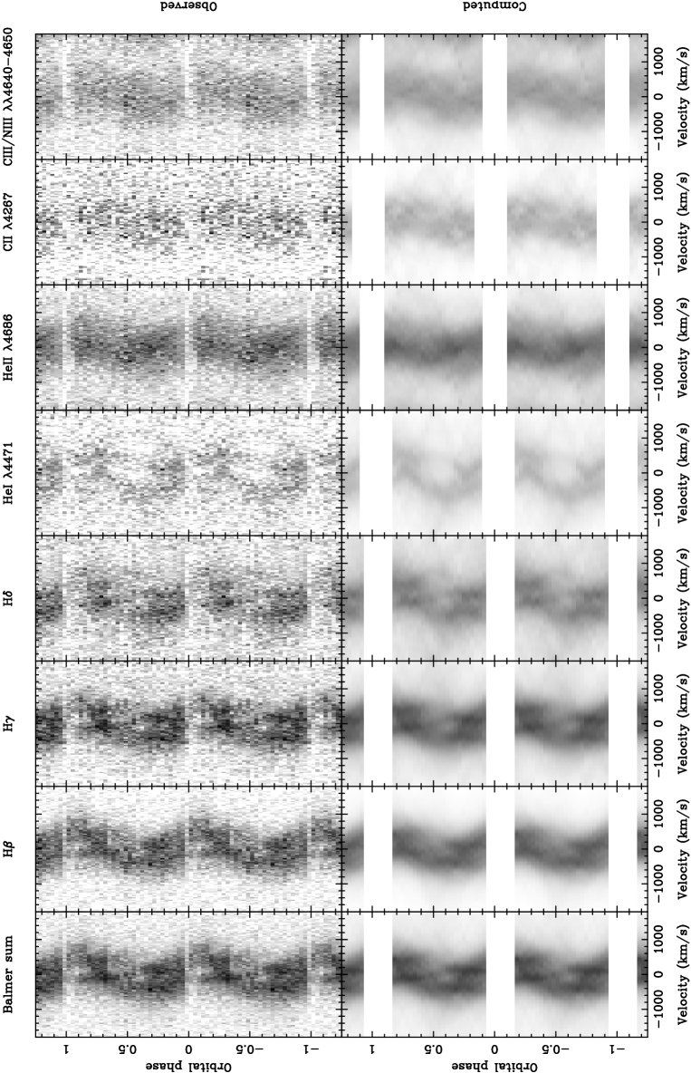
Figure 5: Upper panel – trailed spectra of the sum of the Balmer lines, H$\beta$, H$\gamma$, H$\delta$, He I $\lambda$4471 Å, He II $\lambda$4686 Å, C II $\lambda$4267 Å and C III/N III $\lambda$4640–4650 Å in SW Sex. Lower panel – computed data from the Doppler maps of the above emission lines presented in Fig. 8. The gaps correspond to eclipse spectra which were omitted from the fit. Note that the data have been folded in order to display more than one binary cycle.

4.6 Trailed spectra

We binned the data into 30 binary phase bins and subtracted the continuum from each spectrum using a third-order polynomial fit. We then rebinned the data on to a constant velocity interval scale of 35 km s^-1 pixel^-1, centred on the H$\beta$, H$\gamma$, H$\delta$, He I $\lambda$4471 Å, He II $\lambda$4686 Å, C II $\lambda$4267 Å and C III/N III $\lambda$4640–4650 Å lines. The trailed spectra of these lines are shown in the upper panel of Fig. 5, along with the trailed spectra of the sum of the Balmer lines (computed by taking the weighted average of the three Balmer lines H$\beta$:H$\gamma$:H$\delta$ as 0.41:0.35:0.24). Note that the data have been folded so as to display more than one binary cycle.

The trailed spectra of SW Sex appear to show a number of clearly-defined components. The most dominant is a strong orbital modulation with a semi-amplitude of $\sim 500$ km s^-1 which crosses zero velocity from red to blue at phase $\sim$0.15. This feature appears to be present in all of the emission lines (in the high-excitation features it appears to be the only component) and shares the velocity and phasing of what one might expect of the bright spot. There is a second, lower-velocity component which can only be made out in the Balmer lines, and is particularly well-defined in the plot of the sum of the Balmer lines. This modulation has a semi-amplitude of $\sim 200$ km s^-1 and appears to be in approximate anti-phase to the dominant modulation, crossing zero velocity from blue to red at phase $\sim$0. The most likely origin of this emission is, therefore, the secondary star. There is also evidence for a third component in the Balmer lines, which is most readily apparent at a velocity of $\sim 400$ km s^-1 at phase 0.75 and which appears to be associated with what might be a faint double-peaked accretion disc component. This component is also visible in He I $\lambda$4471 Å. Note that the three emission components we have identified in the trailed spectra all appear to be eclipsed by similar amounts around phase 0 and attenuated by similar amounts around phase 0.5. A further discussion of the various emission regions in SW Sex is deferred until section 4.8, where we report on the results of our Doppler tomography experiments.

4.7 Radial velocities

Figure 6: Radial velocity curves of H$\beta$, H$\gamma$, H$\delta$, He II $\lambda$4686 Å, C III/N III $\lambda$4640–4650 Å, He I $\lambda$4471 Å and C II $\lambda$4267 Å in SW Sex, measured using a double-Gaussian separation of 1600 km s^-1. Points marked by open circles were not included in the fits due to measurement uncertainties during primary eclipse. The horizontal dashed lines represent the systemic velocities. Note that the data have been folded in order to display more than one binary cycle.

A measure of the radial velocity semi-amplitudes of either or both the white dwarf and secondary star is essential in order to derive the component masses of SW Sex. We measured radial velocities of the emission lines in SW Sex by applying the double-Gaussian method of schneider80 to the data presented in the upper panel of Fig. 5. This technique is most sensitive to the motion of the line wings and should thus reflect the radial velocity semi-amplitude of the white dwarf, $K_{W}$, with the highest reliability. The Gaussians were of width 200 km s^-1 ($\sigma$) and we varied their separation from 600 to 2200 km s^-1. We then fitted

$$V=\gamma-K\sin(\phi-\phi_{0})$$ (5)

to each set of measurements, where $V$ is the radial velocity, $K$ is the semi-amplitude, $\phi$ is the orbital phase and $\phi_{0}$ is the phase where the radial velocity curve crosses from red to blue. We omitted four points around phase 0 during the fitting procedure owing to measurement uncertainties during primary eclipse.

Figure 7: Diagnostic diagrams for SW Sex. The left-hand panel shows the results of the radial velocity fits to H$\beta$ (circles connected by solid lines), H$\gamma$ (triangles connected by dashed lines) and H$\delta$ (squares connected by dotted lines). The right-hand panel shows the results of the radial velocity fits to He I $\lambda$4471 Å (diamonds connected by solid lines), He II $\lambda$4686 Å (squares connected by dashed lines), C II $\lambda$4267 Å (crosses connected by dotted lines), and C III/N III $\lambda$4640–4650 Å (stars connected by dashed-dotted lines).

Examples of the radial velocity curves obtained using Gaussian separations of 1600 km s^-1 are shown in Fig. 6. The most striking feature exhibited by these radial velocity curves are the phase shifts, where (with the exception of the relatively noisy He I $\lambda$4471 Å and C II $\lambda$4267 Å curves) the spectroscopic conjunction of each line, i.e. the superior conjunction of the emission line source, occurs after photometric conjunction, i.e. photometric mid-eclipse. This phase shift implies an emission line source trailing the accretion disc, such as the bright spot, and has been observed in other SW Sex stars (e.g. DW UMa, shafter88; V1315 Aql, dhillon91). There is also some evidence of a rotational disturbance in the emission lines of SW Sex during eclipse, as it can be seen that radial velocities measured just prior to eclipse are skewed to the red and those measured just after eclipse are (arguably) skewed to the blue. This confirms the detection of a similar feature in the trailed spectra of Fig. 5 and indicates that at least part of the line emission may originate in an accretion disc.

The final results of the radial velocity analysis are displayed in the form of a diagnostic diagram [Shafter, Szkody & Thorstensen1986] in Fig. 7. By plotting $K$, its associated fractional error $\sigma_{K}/K$, $\gamma$ and $\phi_{0}$ as functions of the Gaussian separation, it is possible to select the value of $K$ which most closely matches $K_{W}$. If there is disc emission contaminated by bright-spot emission, for example, one would expect the solution for $K$ to asymptotically approach $K_{W}$ when the Gaussian separation becomes sufficiently large. Furthermore, since the phasing of the bright-spot is not the same as the white dwarf, one would expect $\phi_{0}$ to approach 0 as the Gaussian separation increases. In order to determine the maximum useful value of the Gaussian separation, one can inspect the fractional error ($\sigma_{K}/K$) curve for an increase, which indicates that the measurements are beginning to be dominated by noise. Taking the results for the Balmer lines in SW Sex first (left-hand panel of Fig. 7), the point where the fractional error starts increasing is at a Gaussian separation of 1600 km s^-1. This means that $K$ is always greater than $\sim 200$ km s^-1, regardless of the Gaussian separation. As pointed out by shafter88, who noted a similar value in DW UMa, this value is distressingly high, implying a very low white dwarf mass. It is clear from the $\phi_{0}$ curves, however, that these $K$-values cannot possibly represent the white dwarf, as even at large Gaussian separations $\phi_{0}\sim 0.1$, implying that nearly all of the line emission must originate from a source, such as the bright-spot, which trails the accretion disc. Clearly, one cannot adopt a reliable value of $K_{W}$ from an analysis of the Balmer emission. The same can also be said for the higher-excitation species displayed in the right-hand panel of Fig. 7, which behave in a largely similar fashion to the Balmer lines, except that they seem to show lower $K$-velocities and larger $\gamma$-velocities. Note that we also attempted to use the light centre technique of marsh88a to determine $K_{W}$, but do not report on the results here as the method was clearly unsuitable to this dataset (as was also found to be the case for V1315 Aql; dhillon91).

4.8 Doppler tomography

The velocity profile of a line observed at a given binary phase is simply the projection of the system’s velocity field on to the line of sight. The orbital motion of the system provides projections along different lines of sight, and thus the velocity field can be recovered from the trailed spectra. This technique is known as Doppler tomography. Full technical details of the method are given by marsh88b and [Horne1991] and an example of its application to real data is given by kaitchuck94.

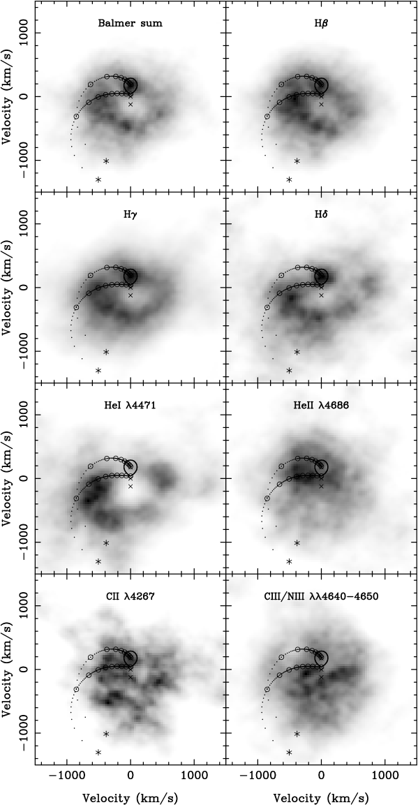
Figure 8: Doppler maps of the sum of the Balmer lines, H$\beta$, H$\gamma$, H$\delta$, He I $\lambda$4471 Å, He II $\lambda$4686 Å, C II $\lambda$4267 Å and C III/N III $\lambda$4640–4650 Å in SW Sex. The three crosses in each map are, from top to bottom, the centres of mass of the secondary, the system and the white dwarf. The predicted outline of the secondary star is marked along with the gas stream and the Keplerian velocity of the disc along the gas stream (the lower and upper curves, respectively). The series of small circles along the gas streams mark the distance from the white dwarf at intervals of $0.1L_{1}$, ranging from $1.0L_{1}$ at the secondary star to the point of closest approach (marked by an asterisk).

Fig. 8 shows the Doppler maps of the sum of the Balmer lines, H$\beta$, H$\gamma$, H$\delta$, He I $\lambda$4471 Å, He II $\lambda$4686 Å, C II $\lambda$4267 Å and C III/N III $\lambda$4640–4650 Å. The maps have been computed from the trailed spectra presented in the upper panel of Fig. 5, with the exception of He II $\lambda$4686 Å and C III/N III $\lambda$4640–4650 Å, which are blended and were thus computed together (see marsh88b). The three crosses marked on each Doppler map represent the centres of mass of the secondary (upper cross), the system (central cross) and the primary (lower cross). The predicted trajectory of the gas stream and the Keplerian velocity of the disc along the gas stream have also been plotted (the lower and upper of the two curves, respectively), along with the secondary’s Roche lobe. These have been computed using representative, but realistic, system parameters of $q=0.7$ and $K_{R}+K_{W}=300$ km s^-1 (see section 4.9). The series of small circles along the gas streams mark the distance from the white dwarf at intervals of $0.1L_{1}$, ranging from $1.0L_{1}$ at the secondary star to the point of closest approach (marked by an asterisk). The lower panel in Fig. 5 shows the data computed from the Doppler maps of Fig. 8; a comparison of the upper and lower panels of Fig. 5 gives some indication of the quality of the fit. The gaps in the computed data correspond to eclipse spectra (defined for each line by the shape of the eclipse light curve in Fig. 4) which have been omitted from the fit as Doppler tomography cannot properly account for obscuration of line-emitting material.

The Balmer-line Doppler maps appear to be dominated by emission from three components – the secondary star, the accretion disc and an extended bright spot. The accretion disc manifests itself as a ring-like structure in the maps, centred on the white dwarf and with a radius of $\sim 500$ km s^-1. If this velocity represents the outer disc velocity, then the radius of the accretion disc would be $R_{D}\sim 0.6L_{1}$ (assuming a representative, but realistic, mass ratio of $q=0.7$; see section 4.9), in good agreement with the photometric determination of the disc radius presented in section 4.2. Superposed on the ring-like disc emission in the Balmer-line maps is a bright spot which has a velocity close to (but not exactly equal to) the expected velocity of the gas stream at a distance from the white dwarf of $\sim 0.5L_{1}$, in reasonable agreement with the disc radius determinations just described. Of course, the precise location of this emission region with respect to the gas stream depends on the system parameters adopted. The bright spot appears much more strongly in the H$\beta$ map than in the H$\gamma$ and H$\delta$ maps and gives the visual impression of line emission originating from the bright spot but extending downstream along the disc edge. The Balmer line maps also display prominent emission from the secondary star, which becomes more dominant relative to the bright spot and disc emission as one moves from H$\beta$ to H$\delta$. The map of He I $\lambda$4471 Å appears similar to the Balmer-line maps but shows no evidence of secondary star emission. The map of He II $\lambda$4686 Å, appears to show only one emission-line source, located with a velocity equal to the gas stream at a distance from the white dwarf of $\sim 0.5L_{1}$ and hence also most likely associated with the bright spot. There is also some evidence that the emission is extended along the gas stream to even greater distances from the white dwarf. Whereas the Balmer-line emission from the bright-spot is not quite coincident with the velocity of the gas stream (assuming our representative system parameters), the He II $\lambda$4686 Å emission lies almost exactly on the expected velocity of the stream and shows no evidence for an extension along the disc rim.

4.9 System parameters

Figure 9: Constraints on the component masses of SW Sex. The white dwarf mass is plotted as a function of the secondary star mass for representative values of $K_{R}$ and the mass-radius relation parameter $b$. Loci of constant inclination (and constant mass ratio) are shown as dashed lines. The horizontal dotted line indicates the Chandrasekhar limit on the mass of the white dwarf. The lines marked with $b=1$ and $b=1.5$ represent secondaries having a mean density near the main sequence and less than the main sequence, respectively.

The radial velocity analysis described in section 4.7 and the Doppler maps presented in Fig. 8 highlight the dangers of using emission lines in CVs to determine the motion of the white dwarf due to the presence of contaminating emission sources. The system parameters of SW Sex derived in this manner by penning84, $M_{1}=0.58\pm 0.20M_{\odot}$ and $M_{2}=0.33\pm 0.06M_{\odot}$, must therefore be viewed as highly dubious. We are fortunate in SW Sex, however, to have detected emission from the secondary star in the Doppler maps. This emission is most likely produced by irradiation of the inner face of the secondary by the accretion disc or bright-spot, as has been observed in DW UMa (dhillon94; rutten94). As the radial velocity of the inner face of the secondary about the centre of mass of the system will be lower than the radial velocity of the centre of mass of the secondary, a measurement of the velocity of the emission feature from the Doppler map can be used to set a lower limit to the true radial velocity semi-amplitude of the secondary, $K_{R}$. From the Doppler map of the sum of the Balmer lines shown in Fig. 8, we find $K_{R}>180$ km s^-1.

We can now place limits upon the system parameters of SW Sex. Following the method outlined by shafter84, it is necessary to solve two $q$ versus $i$ relations using our derived values of $K_{R}$, $P$ and $\Delta\phi_{1/2}$. One $q$ versus $i$ relation is obtained by combining equations (1) and (2). The second $q$ versus $i$ relation is derived by combining the mass function of the secondary star,

$$M_{2}=q^{3}(1+1/q)^{2}PK_{R}^{3}/(2\pi G\sin^{3}{i}),$$ (6)

with Kepler’s third law and a power-law mass-radius relation for the secondary of the form

$$R_{2}/R_{\odot}=b(M_{2}/M_{\odot})^{x},$$ (7)

where the parameters $b$ and $x$ have been determined empirically by patterson84, who finds that $b=1$ and $x=0.88$ for the lower main-sequence.

The results of the preceeding analysis applied to SW Sex are shown in Fig. 9. The white dwarf mass is plotted as a function of the secondary star mass for various values of $K_{R}$ and the mass-radius relation parameter $b$ (adopting $x=0.88$, $\Delta\phi_{1/2}=0.098$ and $P=0.1349384229$ d). Loci of constant inclination (and constant mass ratio) are shown as dashed lines. The horizontal dashed line indicates the Chandrasekhar limit on the mass of the white dwarf. The lines marked with $b=1$ and $b=1.5$ represent secondaries having mean densities near the main sequence and less than the main sequence, respectively. It is clear from Fig. 9 that, without a reliable estimate of $K_{R}$ and the mass-radius relation of the secondary, it is impossible to obtain tight constraints on the masses. By adopting the limit $K_{R}>180$ km s^-1, however, we can say that the secondary mass must be below $\sim 0.3M_{\odot}$ and the primary mass must lie in the range $\sim 0.3-0.7M_{\odot}$. If the secondary is less dense than a main-sequence star, these limits become more severe.

5 Discussion

The literature on the SW Sex phenomenon has been rapidly expanding in recent years. The original theory of an accretion disc wind (honeycutt86) and its variants (dhillon95b; murray96) have been followed by theories of Stark broadening [Lin, Williams & Stover1988], magnetically driven inflows [Williams1989], outflows (tout93; wynn95) and bright-spot overflows (hellier94; hellier96). Judging by the results of our Doppler tomography experiments (section 4.8), it seems that, in the case of SW Sex at least, a much more simple model will suffice. We have identified three emission components, the secondary star, accretion disc and an extended bright spot. In this model, it is the dominance of single-peaked line emission from the bright spot over the weak double-peaked disc emission which gives SW Sex its single-peaked profiles. It is also this dominance which forces the radial velocity curves to follow the motion of the bright spot and thus exhibit large phase shifts. The transient absorption features in the Balmer-line profiles are mostly artifacts of the complex intertwining of the emission components from the secondary star, bright spot and accretion disc and involve little true absorption. While we are confident of the accretion disc and secondary star components of this model, we are less certain of the dominant bright-spot component as it appears to be inconsistent with the emission-line light curves. We discuss why this is the case in section 5.4, but turn first to a more detailed description of the three emission components of our model.

5.1 Balmer emission from the secondary star

Emission from the inner face of the secondary in nova-likes is not uncommon. To date, it has been seen in MV Lyr [Schneider, Young & Shectman1981], TT Ari [Shafter et al.1985], IX Vel [Beuermann & Thomas1990], RW Sex [Beuermann, Stasiewski & Schwope1992], DW UMa (dhillon94; rutten94), UX UMa [Kaitchuck et al.1994], RW Tri [Still, Dhillon & Jones1995], PG 0859+415 [Still1996] and V347 Pup [Still, Buckley & Garlick1997]. Its detection in SW Sex is unusual in that it appears to have been detected while SW Sex was in a normal state (judging by the flux levels in our data when compared with those of still95), whereas most previous detections of the secondary in nova-likes typically occur during periods of low (e.g. DW UMa) or high (e.g. RW Tri) mass transfer. Furthermore, observations of SW Sex obtained two years after the observations presented in this paper also show evidence for secondary star emission [Marsh & Dhillon1997], implying that this is probably not a transient feature. The most likely cause of the emission is irradiation of the inner hemisphere of the secondary by ultraviolet light from the bright spot, accretion disc or boundary layer, although chromospheric emission from the rapidly rotating, late-type secondary cannot be ruled out. With higher signal-to-noise data it should be possible to discriminate between these sources of emission by searching for asymmetries in the distribution of the Balmer emission on the surface of the secondary as one might expect, for example, if the emission were due to irradiation by the bright-spot. As there is no evidence for any He II emission from the secondary we may conclude that soft X-rays from the boundary layer are either not produced or are absorbed by the disc. It should be noted that irradiation of the secondary star in CVs is now seen as a possible contributor to the long-term evolution of CVs (see kolb96 and references therein).

5.2 Balmer and He I emission from the accretion disc

Unambiguous evidence for line emission from the discs of nova-like variables is not as common as one might think. Few nova-likes show double-peaked Balmer or He I emission lines and, to the best of our knowledge, no nova-likes show double-peaked He II $\lambda$4686 Å emission. Similarly, few high-inclination nova-likes show clear evidence for a rotational disturbance during primary eclipse in any of the emission lines. One possible reason for this is that the high mass transfer rates of nova-likes inferred from eclipse maps imply that the discs are largely optically thick in the continuum (rutten92b; williams80). Balmer line-emission from the disc will then come from a relatively small region at the edge of the disc which is optically thin in the continuum, resulting in lines which are narrow, double-peaked and weak. This is precisely what is observed in the disc component of SW Sex and probably accounts for the rarity of the disc component in other nova-likes (where emission from the $(-V_{x},-V_{y})$ quadrant of Doppler maps invariably dominates – see below).

5.3 Line emission from the extended bright-spot

Balmer, He I and He II emission from the $(-V_{x},-V_{y})$ quadrant of Doppler maps seems to be a ubiquitous feature of nova-like variables [Kaitchuck et al.1994]. This emission is not often associated with the bright spot, however, as it has a velocity which is usually too large in the $-V_{y}$ direction. In the case of SW Sex, it appears as if some of the emission does share the velocity of the bright spot, although most of it is still too large in the $-V_{y}$ direction. One possibility is that the latter emission is actually due to post-shock material downstream (along the disc edge) from the point where the gas stream strikes the disc, as has recently been suggested for the short-period dwarf nova WZ Sge [Spruit & Rutten1997]. The resulting line emission, due to recombination as the post-shock material cools down, would share the velocity of the outer edge of the disc. This then provides an explanation for the velocities in the extended bright-spot region of SW Sex displayed in the Doppler maps of Fig. 8, although a detailed radiative hydrodynamical calculation of the shock and post-shock regions would be required to have confidence in such a model. Another possibility is that the extended nature of the bright-spot emission in SW Sex is due to a bright-spot overflow, as suggested for V1315 Aql by hellier96. We believe this is unlikely, however, as one might then expect the emission to follow the gas stream towards higher velocities on the Doppler map, unless interaction with the disc is strong, in which case the emission would be deflected in the $+V_{y}$ direction (towards the curve indicating the Keplerian velocity of the disc along the gas stream in Fig. 8).

5.4 The SW Sex phenomenon explained?

The three-component model outlined above appears to have had some success in explaining much of the behaviour exhibited by SW Sex. We are confident that the accretion disc and secondary star components are correct, but find that the dominant bright-spot component fails in one important area: its inconsistency with the emission-line light curves. This can most readily be seen by inspecting the light curve of H$\gamma$ in Fig. 4, where the eclipse profile requires material to be eclipsed as early as phase 0.8, but which is not as deeply eclipsed as the continuum, exhibits a flat bottom and then comes out of eclipse very sharply around phase 0.05. The early ingress of the light curve (between phases $\sim 0.8-0.9$) cannot be due to obscuration by the secondary star, as the Roche lobe does not eclipse any part of the disc during these phases. Instead, we attribute this to a raised disc rim downstream from the bright-spot, as observed in the dwarf nova OY Car [Billington et al.1996], which passes across the line of sight at this phase and which obscures the disc behind it. The rapid egress between phases 0.01 and 0.05, however, is difficult to explain with a dominant bright-spot component as one would expect it to be obscured by the secondary at these phases (for any reasonable set of system parameters). For the same reason, it is also difficult to explain the general reduction in line flux observed around phase 0.5. It is still possible to account for the emission-line light curves with a dominant bright-spot component, however, by speculating that there are regions of strong Balmer absorption in the disc whose changing visibility during eclipse alters the shape of the light curve. Alternatively, we might invoke some of the more exotic theories of the past in which there is a source of Balmer emission from above the orbital plane of the binary, although this would still have to share the velocity of the bright-spot.

References

- [\citefmtAshoka et al.1994] Ashoka B. N., Seetha S., Marar T. M. K., Kasturirangan K., Rao U. R., Bhattacharyya J. C., 1994, A&A, 283, 455
- [\citefmtBeuermann & Thomas1990] Beuermann K., Thomas H.-C., 1990, A&A, 230, 326
- [\citefmtBeuermann, Stasiewski & Schwope1992] Beuermann K., Stasiewski U., Schwope A. D., 1992, A&A, 256, 433
- [\citefmtBillington et al.1996] Billington I., Marsh T. R., Horne K., Cheng F. H., Thomas G., Bruch A., O’Donoghue D., Eracleous M., 1996, MNRAS, 279, 1274
- [\citefmtDhillon & Rutten1995] Dhillon V. S., Rutten R. G. M., 1995, MNRAS, 277, 777
- [\citefmtDhillon, Jones & Marsh1994] Dhillon V. S., Jones D. H. P., Marsh T. R., 1994, MNRAS, 266, 859
- [\citefmtDhillon, Marsh & Jones1991] Dhillon V. S., Marsh T. R., Jones D. H. P., 1991, MNRAS, 252, 342
- [\citefmtDhillon et al.1992] Dhillon V. S., Marsh T. R., Jones D. H. P., Smith R. C., 1992, MNRAS, 258, 225
- [\citefmtDhillon1996] Dhillon V. S., 1996, in Evans A., Wood J. H., eds, Cataclysmic Variables and Related Objects. Kluwer Academic Publishers, Dordrecht, p. 3
- [\citefmtEggleton1983] Eggleton P. P., 1983, ApJ, 268, 368
- [\citefmtGreen et al.1982] Green R. F., Ferguson D. H., Liebert J., Schmidt M., 1982, PASP, 94, 560
- [\citefmtGreen, Schmidt & Liebert1986] Green R. F., Schmidt M., Liebert J., 1986, ApJS, 61, 305
- [\citefmtHarrop-Allin & Warner1996] Harrop-Allin M. K., Warner B., 1996, MNRAS, 279, 219
- [\citefmtHellier & Robinson1994] Hellier C., Robinson E. L., 1994, ApJ, 431, L107
- [\citefmtHellier1996] Hellier C., 1996, ApJ, 471, 949
- [\citefmtHoneycutt, Schlegel & Kaitchuck1986] Honeycutt R. K., Schlegel E. M., Kaitchuck R. H., 1986, ApJ, 302, 388
- [\citefmtHorne & Marsh1986] Horne K., Marsh T. R., 1986, MNRAS, 218, 761
- [\citefmtHorne1991] Horne K., 1991, in Shafter A. W., ed, Proceedings of the 12th North American Workshop on Cataclysmic Variables and Low Mass X-ray Binaries. SDSU Press, San Diego, p. 23
- [\citefmtJorden & Fordham1986] Jorden A. R., Fordham J. L. A., 1986, QJRAS, 27, 166
- [\citefmtKaitchuck et al.1994] Kaitchuck R. H., Schlegel E. M., Honeycutt R. K., Horne K., Marsh T. R., White J. C., Mansperger C. S., 1994, ApJS, 93, 519
- [\citefmtKolb1996] Kolb U., 1996, in Evans A., Wood J. H., eds, Cataclysmic Variables and Related Objects. Kluwer Academic Publishers, Dordrecht, p. 433
- [\citefmtLin, Williams & Stover1988] Lin D. N. C., Williams R. E., Stover R. J., 1988, ApJ, 327, 234
- [\citefmtMarsh & Dhillon1997] Marsh T. R., Dhillon V. S., 1997, MNRAS, submitted
- [\citefmtMarsh & Duck1996] Marsh T. R., Duck S. R., 1996, New Astronomy, 1, 97
- [\citefmtMarsh & Horne1988] Marsh T. R., Horne K., 1988, MNRAS, 235, 269
- [\citefmtMarsh1988] Marsh T. R., 1988, MNRAS, 231, 1117
- [\citefmtMassey et al.1988] Massey P., Strobel K., Barnes J. V., Anderson E., 1988, ApJ, 328, 315
- [\citefmtMurray & Chiang1996] Murray N., Chiang J., 1996, Nature, 382, 789
- [\citefmtPatterson1984] Patterson J., 1984, ApJS, 54, 443
- [\citefmtPenning et al.1984] Penning W. R., Ferguson D. H., McGraw J. T., Liebert J., Green R. F., 1984, ApJ, 276, 233
- [\citefmtPringle1975] Pringle J. E., 1975, MNRAS, 170, 633
- [\citefmtPringle1981] Pringle J. E., 1981, ARA&A, 19, 137
- [\citefmtRutten & Dhillon1994] Rutten R. G. M., Dhillon V. S., 1994, A&A, 288, 773
- [\citefmtRutten et al.1993] Rutten R. G. M., Dhillon V. S., Horne K., Kuulkers E., van Paradijs J., 1993, Nature, 362, 518
- [\citefmtRutten, van Paradijs & Tinbergen1992] Rutten R. G. M., van Paradijs J., Tinbergen J., 1992, A&A, 260, 213
- [\citefmtRutten1997] Rutten R. G. M., 1997, A&A, submitted
- [\citefmtSchneider & Young1980] Schneider D. P., Young P. J., 1980, ApJ, 238, 946
- [\citefmtSchneider, Young & Shectman1981] Schneider D. P., Young P. J., Shectman S. A., 1981, ApJ, 245, 644
- [\citefmtShafter, Hessman & Zhang1988] Shafter A. W., Hessman F. V., Zhang E. H., 1988, ApJ, 327, 248
- [\citefmtShafter et al.1985] Shafter A. W., Szkody P., Liebert J., Penning W. R., Bond H. E., Grauer A. D., 1985, ApJ, 290, 707
- [\citefmtShafter, Szkody & Thorstensen1986] Shafter A. W., Szkody P., Thorstensen J. R., 1986, ApJ, 308, 765
- [\citefmtShafter1984] Shafter A. W., 1984, AJ, 89, 1555
- [\citefmtSpruit & Rutten1997] Spruit H. C., Rutten R. G. M., 1997, A&A, in press
- [\citefmtStill, Buckley & Garlick1997] Still M. D., Buckley D. A. H., Garlick M. A., 1997, MNRAS, in press
- [\citefmtStill, Dhillon & Jones1995] Still M. D., Dhillon V. S., Jones D. H. P., 1995, MNRAS, 273, 849
- [\citefmtStill1995] Still M. D., 1995, PhD thesis, University of Sussex
- [\citefmtStill1996] Still M. D., 1996, MNRAS, 282, 943
- [\citefmtSulkanen, Brasure & Patterson1981] Sulkanen M. E., Brasure L. W., Patterson J., 1981, ApJ, 244, 579
- [\citefmtSzkody & Piché1990] Szkody P., Piché F., 1990, ApJ, 361, 235
- [\citefmtThorstensen et al.1991] Thorstensen J. R., Ringwald F. A., Wade R. A., Schmidt G. D., Norsworthy J. E., 1991, AJ, 102, 272
- [\citefmtTout, Pringle & la Dous1993] Tout C. A., Pringle J. E., la Dous C., 1993, MNRAS, 265, 5p
- [\citefmtWarner1995] Warner B., 1995, Cataclysmic Variable Stars. Cambridge University Press, Cambridge
- [\citefmtWilliams1980] Williams R. E., 1980, ApJ, 235, 939
- [\citefmtWilliams1989] Williams R. E., 1989, AJ, 97, 1752
- [\citefmtWynn, King & Horne1995] Wynn G., King A. R., Horne K., 1995, in Buckley D. A. H., Warner B., eds, Magnetic Cataclysmic Variables. ASP Conference Series, Volume 85, p. 196