The X$-$ray flux and spectral variability of EMSS AGN

Abstract

Fifteen $ROSAT$ PSPC observations available in the public archive are analyzed in order to study time and spectral variability of the 12 EMSS AGN detected by $ROSAT$ with more than 2000 net counts. Time variability was investigated on 13 different time scales, ranging from 400 s to 3.15$\times 10^{6}$ s (1 year). Of the 12 sources analyzed, only two do not show a significant variability on any time scale. On short time scale $\leq$ 20 percent of AGN are seen as variable sources while on time scale of $\geq$100.000 s the fraction becomes $\geq$50 percent. However one should bare in mind that the visibility function for variability is far from being uniform and that small amplitude variations can be detected more often on long time scale than on short time scale. Spectral variability was detected in only two sources. MS1158.6$-$0323 shows an hardening of the spectrum with increasing intensity while MS2254.9$-$3712 shows a softening of the spectrum with increasing intensity. Finally, for one source (MS1416.3$-$1257), the observed variability is not due to an intrinsic flux variation but, instead, to a variation in the column density along the line of sight. Since this variability has been observed on a time scale of $\sim$ 3.9 days, it is probably associated to the broad line clouds.

1 INTRODUCTION

Active Galactic Nuclei (AGN) emit enormous energies over the electro magnetic spectrum bands from radio through gamma rays. In view of their short time variability, it has never been questioned that the power supply is primarily gravitational. The shortest time scales variability is seen at high energy (McHardy 1990, Grandi et al. 1992). Since a substantial variability cannot be observed on a time scale shorter than the light crossing time of the source (R$<$c$\delta$t), the X-ray variability is a powerful probe of the innermost regions of AGN and can be used to constrain the emission mechanisms, the size of the emitting region and the efficiency of the matter/radiation conversion processes.

Long duration, uninterrupted X-ray observations of AGN (hereafter with the term AGN we refer to QSO and Seyfert Galaxies, i.e. emission lines AGN) were first carried out by EXOSAT (White and Peacock 1989), which showed that AGN are X-ray sources with flux changes over a wide range of time scales and that short term X-ray variability, down to a few hundred seconds, is common (McHardy 1990). A reanalysis of the EXOSAT data (Grandi et al. 1992) showed that $\sim$40% of AGN show variability on time scales less than one day. On longer time scales (typically weeks to months) 97% of the same sample showed variability, suggesting than the long time variability is much more common (see also Mushotzky, Done & Pounds 1993).

The EXOSAT and $Ginga$ observations have also made evident that spectral shape changes can accompany luminosity variations. Although the prevailing trend appears to be a softening of the spectrum with increasing intensity, AGN do not show a unique spectral behavior (Grandi et al. 1992). This is in contrast to the results obtained for BL Lac objects, a particular class of AGN which show peculiar characteristics as a featureless optical spectrum, high polarization and rapid variability. Using the EXOSAT data, Giommi et al. (1990) have found that BL Lac show a systematic hardening of the spectrum as the sources brightens.

Recent $ROSAT$ observations have confirmed that the overall picture of the spectral variability is still rather confused. For example Boller et al. (1996) using a sample of narrow-line Seyfert 1 galaxies have found that some objects ($e.g.$ MKN 957) show a softening of the spectrum with increasing intensity, while other sources ($e.g.$ I ZW1, MKN 507) do not show spectral variability associated with flux variations. Moreover, Molendi & Maccacaro (1994) using $ROSAT$ data on MKN 766 have found a complex spectral variability in which the 0.1$-$0.9 keV part of the spectrum hardens as the source brightens while the 0.9$-$2.0 keV part of the spectrum does not change significantly. A detailed description of the expected X-ray variability in the framework of different theoretical models can be found in a recent paper of Haardt, Maraschi and Ghisellini (1997).

Using the enormous quantity of data available in the public $ROSAT$ archive, we started a program aimed at the study of the X-ray properties of X-ray selected AGN. In particular we are using the sample of AGN extracted from the $Einstein$ Extended Medium Sensitivity Survey (Gioia et al. 1990, Stocke et al. 1991, Maccacaro et al. 1994) for which the original available information on the X-ray properties is limited by the poor energy resolution of the IPC and by the limited statistics of the detected sources. In the first paper (Ciliegi & Maccacaro 1996) we have studied the X-ray spectral properties of all the EMSS AGN detected with more than 300 net counts in $ROSAT$ PSPC images available from the public archive. Here we complete our work reporting the flux and spectral variability analysis of the EMSS AGN. In Section 2 we define the sub-sample of EMSS AGN used, while in Section 3 we describe the method of analysis. In Section 4 we report the results for time and spectral variability, while in Section 5 the conclusion are presented.

2 THE SAMPLE

From the sample of Ciliegi & Maccacaro (1996) of 63 EMSS AGN detected by $ROSAT$ with more than 300 measured net counts, we have extracted all the sources detected with more than 2000 net counts. Of the 14 sources satisfying this criteria, two (MS0919.3+5133 and MS1215.9+3005) were excluded from the sample: MS0919.3+5133 was detected near the window support structure, so unreal flux variations may be detected due to the $ROSAT$ wobble and MS1215.9+3005 (MKN 766) was already studied in detail by Molendi et al. (1993) and Molendi & Maccacaro (1994)

Figure 1: Light curves for all the 12 EMSS AGN analyzed. For each observations we report the source light curve obtained with a bin of 3600 s (top panel) and, for comparison, the background light curve (lower panel)

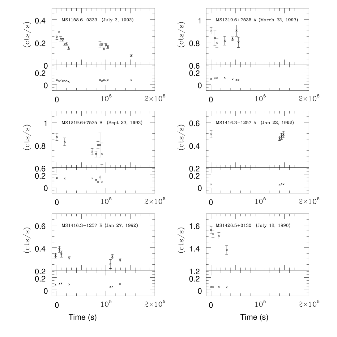
Figure 1: continued

Figure 1: continued

Figure 1: continued

The present sample includes 12 EMSS AGN and is listed in Table 1 which is organized as follows: source name and morphological type (with relative reference within bracket) followed by radio flux, optical magnitude, $Einstein$ X-ray flux, redshift, off-axis angle $\theta$ (the distance between the source and the center of the PSPC field), net counts detected in the 0.1$-$2.4 keV band with the relative error, exposure time, sequence number (ror) and date of the $ROSAT$ observations. Finally in the last column we report a list (incomplete) of references to previous works. We note that for MS1112.5+4059 and MS2254.9-3712 more than one observation is available.

Due to the selection criteria ($\geq$ 2000 net counts) the 12 EMSS sources analyzed here have optical and x-ray fluxes greater than the average of the EMSS sample ($<$m${}_{V}>$ = 17.9; $<$f_x(0.3–3.5 keV)$>$ = 7$\times 10^{-13}$ erg cm^-2 s^-1) and smaller redshifts. They cannot be considered representative of the whole EMSS AGN sample but rather of its bright end.

3 DATA ANALYSIS

For each source we extracted the total counts in the 0.1$-$2.4 keV band using a circle centered on the source centroid. Background counts were estimated in an annulus centered on the source and subtracted from the total counts. A detailed description of data processing and analysis is reported in Ciliegi & Maccacaro (1996).

3.1 Time Variability

Time variability was investigated on 13 different time scales, ranging from 400 s to 3.15$\times 10^{6}$ s (1 year). For all the sources we have binned the data in bins that are an integer multiple of 400 s. We do this to avoid apparent flux variations due to the $ROSAT$ wobble period of about 400 s. Brinkmann et al. (1994) have shown that flux determination in wobble mode is good to within $\sim$ 4 per cent when binning over integer multiples of the 400 s wobble period. Moreover, for each time scale a careful analysis of the background was made to ensure that observed variability is not due to a change in the background rate. The light curve of all the sources obtained with a bin of 3600 s are shown in Figure 1. For each observation we report the source light curve (top panel) and, for comparison, the background light curve (lower panel).

In order to understand and to interpret the properties of flux variability, attention should be paid not only to what has been detected but also to what could or could not have been detected. The capability of detecting a variation of a given amplitude depends on the accuracy of the flux measurement, which itself depends on the total number of detected counts. To quantify this effect, for all the sources we have computed the minimum detectable variation (MDV) at 3 $\sigma$ level in each time scale considered. The MDV has been obtained as follows: for a given time scale, a variation of a fraction K in flux (defined as $\mid$C${}_{i+1}-$C${}_{i}\mid$/C_i) between two consecutive bins can be detected (with a significance level of N $\sigma$) if
$\mid$C${}_{i}-$ C${}_{i+1}\mid>$N$\times\sqrt{E_{i}^{2}+E_{i+1}^{2}}$, where C_i, C_i+1, $E_{i}$ and $E_{i+1}$ are the net counts and the relative errors in the $i$th and in the $i+1$th bin. Writing C_i+1 = C_i(1+K) and assuming $E_{i+1}=E_{i}$(1+K)^1/2 we have:
C_iK $>$ N $\times\sqrt{E_{i}^{2}(1+(1+K))}$ which gives $E_{i}$/C${}_{i}<\sqrt{K^{2}/(N^{2}(1+(1+K))}$.
For example, to be able to detect a variation of 30 per cent (K=0.3) at a significance level of 3 $\sigma$ (N=3), we must have $E_{1}$/C${}_{1}<$ 0.066 in at least two consecutive bin.

3.2 Spectral variability

For the sources that show flux variability we have calculated the hardness ratio HR for each bin of the light curve in order to study a possible correlation between HR and count rate. The hardness ratio provides a powerful tool for the detection of X-ray spectral variability, as the hardness ratio is model independent. The hardness ratio HR is defined as HR=(H$-$S)/(H+S) where S is the number of net counts detected in the 0.11$-$0.43 keV band and H is the number of net counts detected in the 0.50$-$2.02 keV band.

Moreover, in order to carry out a less detailed but statistically more significant analysis, for each source we have divided the $ROSAT$ data into two subsets depending on whether the count rate is below (low state) or above (high state) the mean count rate and we have computed the hardness ratio for each subset. The results of the time and spectral variability analysis are reported in the next Section.

4 Results

For all the time scale considered we have calculated the observed variability (ObV) at the 3 $\sigma$ level for each of the 12 EMSS AGN detected by $ROSAT$ with more than 2000 net counts. The observed variability, calculated between all the consecutive bins, is defined as ObV = $\mid$CR(i+1) - CR(i)$\mid$/CR(i), where CR(i) and CR(i+1) are the observed count rate in the $i$th and in the $i+1$th bin respectively. For each time scale, in Table 2 we report the minimum detectable variability (MDV), the minimum and the maximum value of the observed variability and (within bracket) the number of times that we detected a significant variability at 3 $\sigma$ level.

As shown in the Table, not all the sources have been observed over the same time scales. This is due to the fact that the sampling of the data is fairly heterogeneous. For some sources the sampling is fairly constant over few days, while for other sources is strongly discontinuous with gaps of week or months ($i.e.$ time that the satellite has spent on other sources). We note that over long time scales the detected variability results from the comparison of observations separated by a significant amount of time during which the source was not monitored (see for instance the case of MS2254.9$-$3712, observed on May 2, 1992 and on May 12, 1993). It is clear that the statement that the source has varied over a time scale of one year is true but the one year time scale should be considered as an upper limit. We do not know whether the transition from a lower to a higher count rate occurred smoothly over several months or abruptly in a much shorter time scale.

Of the 12 sources analyzed, only two (MS1059.0+7302 and MS1559.1+3324) do not show a significant variability on any time scale. In Figure 2 we report the fraction of the

Figure 2: The fraction of the sources that show a significant variability as a function of time scale

sources that show a significant variability as a function of the time scale. As clearly shown in Figure 2, long time scale variability is much more common than short time scale variability, in agreement with the results obtained by Grandi et al. (1992) with the EXOSAT data. Table 2 also shows that the typical amplitude of the variability observed on short time scales are, in general, lower than that on long time scales. With few exceptions, the amplitude of the variation on time scale less than 30 hours are always lower than 30 per cent, while on longer time scale the amplitude of the variations are always greater than 30 per cent. Therefore the increasing fraction of variable source on longer time scale is due to the combination of two effects: an increase in the amplitude of the variation and the contemporaneous decrease of the MDV due to the better statistic available on longer time scales.

For the 10 sources that show a significant variability, we also searched for the shortest time scale on which a significant variability occurs. The 10 variable sources are listed in Table 3 where we report the source name, the shortest time scale on which we detected a significant ($>3\sigma$) variability, the percentage flux variation occurred during the shortest time scale (defined as in Table 2) and the corresponding luminosity variation. Assuming that the luminosity is produced by matter being transformed into radiation with some efficiency $\eta$, we have calculate $\eta$ for each source using $\Delta L\leq(\eta$ m_p c⁴ t_var) / $\sigma_{T}$ where $\sigma_{T}$ is the Thomson cross-section and m_p the mass of proton (Fabian 1992). For all the sources the observed luminosity variation imply an efficiency $\eta<$ 0.1, so there is no indication that the observed X-ray radiation is beamed.

Of the 10 sources with detected flux variability, only 3 show also a spectral variation associated with the flux variation. Below we discuss the flux and spectral properties of these three sources.

TABLE 3 : Sources with detected variability

SOURCE	$\Delta T_{\tiny\rm min}$	$\Delta F$	$\Delta L$
	(s)		erg s-1
MS0310.4$-$5543	2.56$\times 10^{6}$	50%	4.02$\times 10^{45}$
MS1112.5+4059	2.16$\times 10^{5}$	40%	2.86$\times 10^{43}$
MS1158.6$-$0323	8000	32%	1.17$\times 10^{42}$
MS1219.6+7535	72000	15%	1.04$\times 10^{44}$
MS1416.3$-$1257	4.32$\times 10^{5}$	33%	3.07$\times 10^{44}$
MS1426.5+0130	14400	17%	2.01$\times 10^{44}$
MS1747.2+6837	40000	56%	1.59$\times 10^{44}$
MS2159.5$-$5713	56000	33%	7.03$\times 10^{43}$
MS2254.9$-$3712	1200	16%	1.25$\times 10^{43}$
MS2340.9$-$1511	1200	16%	2.39$\times 10^{44}$

4.1 Sources which show flux and spectral variability

MS1158.6$-$0323 (MKN 1312)

For this source we detected an X-ray count rate decrease of $\sim$32 per cent on a time scale of 8000 seconds, while over the whole $ROSAT$ observation the ratio of maximum to minimum count rate was $\sim$ 3.6. We searched for spectral variability calculating the hardness ratio in each bin of the light curve. In Figure 3 we report the 3600 s light curve of MS1158.6$-$0323 and, for comparison, the value of the hardness ratio in each bin. Figure 3 shows an hardening of the spectrum as the source brightens, although this trend is not statistically significant (the error bars represent the 1 $\sigma$ error). However, if we divide the data into two subsets from 0.08 to 0.18 counts s^-1 (low state) and from 0.18 to 0.29 counts s^-1 (high state) the hardening of the spectrum becomes significant, with HR${}_{\em LOW~{}STATE}=0.26\pm 0.02$ and HR${}_{\em HIGH~{}STATE}=0.34\pm 0.02$.

Figure 3: The light curve of MS1158.6$-$0323 obtained with a bin of 3600 s (top panel) and the value of the hardness ratio HR in each bin (lower panel)

MS1416.3$-$1257 (PG1416-12)

This source show a significant X-ray count rate decrease of 33 per cent on a time scale of 4.32$\times 10^{5}$ s ($\sim$ 5 days). Therefore we splitted the observation of MS1416.3$-$1257 into two data sets separated by 4.32$\times 10^{5}$ s and we searched for spectral variability. The spectrum in the first data set is well parameterized by fitting the data with a broken power-law with N_H fixed at the Galactic value (6.8$\times 10^{20}$ cm^-2). It yields $\alpha_{x}$=1.20$\pm$0.06 and $\chi^{2}$/dof=20.55/26 with a flux (unabsorbed for Galactic N_H) of 118.3$\pm$3.32 10^-13 erg cm^-2 s^-1 (0.1$-$2.4 keV band). Modeling the data with N_H as a free parameter does not yield a significant improvement to the fit, with $\alpha_{x}$=1.18$\pm$0.21, N_H=6.69${}^{+1.02}_{-0.93}\times 10^{20}$ cm^-2 and $\chi^{2}$/dof=20.53/25.

In the second data set, the spectrum shows excess absorption relative to the Galactic value. In fact, while the model with N_H=N${}_{H~{}Gal}$ yields $\alpha_{x}=1.00\pm 0.11$ and $\chi^{2}$/dof=30.35/21, the model with N_H free to vary yields $\alpha_{x}=1.35\pm 0.23$, N_H=9.7$\pm 1.4\times 10^{20}$ cm^-2 and $\chi^{2}$/dof=17.27/20. The reduction in $\chi^{2}_{FIT}$ with the addition of N_H as a free parameter is statistically significant (P${}_{F>F_{FIT}}$=9.0 10^-4 with F test). The absorption excess can be well parameterized by fitting the data with a power-law ($\alpha_{x}=1.35\pm$0.25) absorbed by Galactic N_H plus a second absorption component (N_H=2.86${}^{+2.19}_{-0.75}\times 10^{20}$ cm^-2) at the redshift of the source (z=0.129). Using this model, the flux of the source, unabsorbed for Galactic N_H and for the second absorption component, is f_x(0.1$-$2.4)=121.3$\pm$3.32 10^-13 erg cm^-2 s^-1, consistent with the flux observed in the first observation. Therefore the observed variability of MS1416.3$-$1257 is not due to a flux variation of the source, but to a variation in the column density.

Variations in the column density are not common events in AGN. They have been seen in only few object like, for example, NGC4151 (Yaqoob et al. 1993), ESO103$-$G55 (Warwick et al. 1988), NGC6814 (Leighly et al. 1992), NGC5506 (Bond et al. 1992). The presence of a significant amount of X-ray column density in AGN is generally associated with the accretion disk, the cold torus, the disk of the galaxy itself (Lawrence and Elvis 1982) or with the broad line clouds. The apparent rarity of variations in absorption is consistent with all these explanations, although the occurrence of variability at all argues for a component associated with either the broad line clouds or the edge of the accretion disk, since the other two regions are not expected to change on observable time scales.

MS2254.9$-$3712

Figure 4: As in Figure 3 for MS2254.9$-$3712

For this source we have 3 different observations (see Table 1). As shown in Figure 1, this source show strong variability both on short and long time scales. A significant increase and decrease of the count rate of $\sim$16 per cent were detected on time scales of 1200 s, while on a time scale of 86800 s the source count rate decreased by a factor of $\sim$3.3.

We searched for spectral variability calculating the hardness ratio in each bin of the light curve. The results are presented in Figure 4 which shows a complex pattern, although the prevailing trend appears to be a softening of the spectrum with increasing intensity. This is confirmed by Figure 5 where we report the hardness ratio HR as a function of count rate. If we divide the data into two subset: from 0.51 to 0.90 counts s^-1 (low state) and from 0.90 to 1.43 counts s^-1 (high state), the softening of the spectrum with increasing intensity becomes significant, with HR${}_{\em LOW~{}STATE}=-0.46\pm 0.01$ and HR${}_{\em HIGH~{}STATE}=-0.53\pm 0.01$

Figure 5: The hardness ratio HR as a function of count rate for MS2254.9$-$3712

5 Conclusions

The flux and spectral variability analysis of a sample of 12 EMSS AGN has confirmed that long term ($\geq$ 30 hours) variability is more common than short term variability. However this effect is probably due to a selection effect more than to a real increase of the fraction of AGN that show a variability. In this respect we note that Fig. 2 shows an increase of the fraction of AGN exhibiting flux variation with increasing time scale. On short time scale about 20 percent or less of AGN are seen as variable sources while on time scale of 100.000 s or more the fraction becomes $\geq$ 50 percent. However one should bare in mind that the visibility function for variability is far from being uniform. Inspection of table 2 shows that small amplitude variations can be detected more often on long time scale than on short time scale.

On the other end we note that, considering only sources for which variability has been detected, on time scale less than 30 hours the amplitude of the variation are mainly lower than 30 per cent while on longer time scale the amplitude are mainly greater than 30 per cent.

Unfortunally, using only the ROSAT data we are not able to determine the very nature of the detected variability and to understand if the different intensity detected on time scale shorter and longer than 30 hours is due to different physical and/or geometrical properties.

As shown by Haardt, Maraschi and Ghisellini (1997), the only way to determine the real nature of an observed X-ray variability is an accurate analysis of the flux variability as a function of the spectral variability in the 2$-$10 keV band together with simultaneous observation in the 0.1$-$2.0 keV band.

However, it is interesting to note that a time scale of 30 hours corresponds to an upper limit to the size of the source (R$\leq$c$\delta$t) of $\sim$ 3$\times 10^{15}$ cm. In the most accepted picture of the physical structure of AGN (see, for example, Urry and Padovani 1995), this region is between the accretion disk around the central black hole ($\sim 1-30\times 10^{14}$ cm for a central black hole of 10⁸M_⊙) and the region of the broad line clouds ($\sim 2-20\times 10^{16}$ cm). Therefore, while the variability on time scale shorten than 30 hours is surely associated with a variation in the accretion disk, on longer time scale it can arise from larger regions where other factors ($i.e.$ scattered radiation, absorbing clouds) can contribute to the observed variability.

For one source (MS1416.3$-$1257) the observed variability is not due to a flux variation but, instead, to a variation in the column density along the line of sight. Since this variability has been observed on a time scale of $\sim$ 3.9 days, it is probably associated to the broad line clouds.

Spectral variability was detected in only two sources. MS1158.6$-$0323 shows an hardening of the spectrum with increasing intensity while MS2254.9$-$3712 shows a softening of the spectrum with increasing intensity. Finally MS1215.9+3005 (MKN766), which was excluded from our analysis because already studied in detail by Molendi and Maccacaro (1994) but is part of the selected sample, shows a different behavior between the soft (0.1-0.9 keV) and hard (0.9-2.0 keV) part of the spectrum. The soft part harden as the source brightens while the hard part does not change significantly. These results confirm that the overall picture of the flux and spectral variability is still rather confused. An improvement of our knowledge in this field should come from the data of the recently launched XTE and SAX X-ray satellite and from the forthcoming AXAF and XMM missions, characterized by the possibility of long, uninterrupted observations over a broader energy band.

References

- [1] Boller T., Brandt W.N. and Fink H., 1996, A&A, 305, 53.
- [2] Bond I., Matsuoka M. and Yamauchi M., 1992, ApJ, 405, 179.
- [3] Bowyer S., Lampton M., Lewis J., Wu X., Jelinsky P. and Mailina R.F., 1996, ApJS, 102, 129.
- [4] randt W.N, Fabian A.C., Nandra K., Reynolds C.S. and Brinkmann W., 1994, MNRAS, 271, 958.
- [5] Brinkmann W.N. et al., 1994, A&A, 288, 433.
- [6] Ceballos M.T. and Barcons X., MNRAS, 282, 493.
- [7] Ciliegi P. and Maccacaro T., 1996, MNRAS, 282, 477.
- [8] Cordova F.A., Kartje J.F., Thompson Jr. R.J., Mason K.O., Puchnarewicz E.M. and Harnden Jr. F.R., 1992, ApJS, 81, 661.
- [9] Elvis M. et al., 1994, ApJS, 95, 1.
- [10] Fabian A.C., 1992, in Brinkmann W., Trümper J., eds, X-ray Emission from Active Galactic Nuclei and the Cosmic Background, MPE Report 235, p. 22.
- [11] Fiore F., Elvis M., McDowell J., Siemiginowska A. and Wilkes., 1994, ApJ, 431, 515.
- [12] Fiore F., Elvis M., Siemiginowska A., Wilkes B.J, McDowell J. and Mathur S., 1995, ApJ, 449, 74.
- [13] Fruscione A., 1996, ApJ, 459, 509.
- [14] Gioia I.M., Maccacaro T., Schild R.E., Wolter A., Stocke J.T., Morris S.L., and Henry J.P., 1990, ApJS, 72, 567.
- [15] Giommi P., Barr P., Garilli B.,Maccagni D. and Pollock A.M.T., 1990, ApJ, 356, 432.
- [16] Giommi P. et al., 1991, ApJ, 378, 77.
- [17] Grandi P., Tagliaferri G., Giommi P., Barr P. and Palumbo G., 1992, ApJS, 82, 93.
- [18] Haardt F., Maraschi L. and Ghisellini G., 1997, ApJ, in press.
- [19] Hewitt A. and Burbidge G., 1991, ApJS, 75, 297.
- [20] Laurikainen E., Salo H., Teerikorpi P. and Petrov G., 1994, A&AS, 1bib08, 491.
- [21] Lanzetta K.M, Turnshek D.A and Sandoval J., 1993, ApJS, 84, 109.
- [22] Lawrence A. and Elvis M., 1982, ApJ, 256, 410.
- [23] Leighly K., Kunieda H and Tsuruta S., 1992, in Testing the AGN Pbibaradigm, New York: Am.Inst.Phys., p. 93.
- [24] Maccacaro T., Wolter A., McLean B., Gioia I.M., Stocke J.T., Della Ceca R., Burg R. and Faccini R., 1994, Astrophysical Letters and Communications, 29, 267.
- [25] McHardy I., 1990, in X-ray Astronomy (Proc. 23d ESLAB Symposium) ed. N.E. White, 2, 1111.
- [26] Molendi S. and Maccacaro T., 1994, A&A, 291, 420.
- [27] Molendi S., Maccacaro T. and Schaeidt S., 1993, A&A, 271, 18.
- [28] Mushotzky R.F., Done C. and Pounds K.A., 1993, ARA&A, 31, 717.
- [29] Puchnarewicz E.M., Mason K.O., Cordova F.A., Kartje J., Branduardi-Raymont G., Mittaz J.P.D., Murdin P.G. and Allington-Smith J., 1992, MNRAS, 256, 589.
- [30] Rafanelli P., Violato M. and Baruffolo A, 1995, ApJ, 439, 90.
- [31] Rowan-Robinson M., 1995, MNRAS, 272, 737.
- [32] Rush B., Malkan M.A. and Edelson R.A., 1996, ApJ, 473, 130.
- [33] Siemiginowska A., Kuhn 0., Elvis M., Fiore F., McDowell J. and Wilkes B.J., 1995, ApJ, 454, 77.
- [34] tocke J.T., Morris S.L., Gioia I.M., Maccacaro T., Schild R.E., Wolter A., Fleming T.A., and Henry J.P., 1991, ApJS, 76, 813.
- [35] Urry C.M. and Padovani P., 1995, PASP, 107, 803.
- [36] Walter R. and Fink H., 1993, A&A, 274, 105.
- [37] Warwick R.S., Pounds K.A. and Turner T., 1988, MNRAS, 231, 1145.
- [38] White N.E. and Peacock A., 1989, in X-ray Astronomy with , ed. N.E. White and R. Pallavicini (Mem. Soc. Astron. Ital., 59), 7.
- [39] Yaqoob T., Warwich R.S., Makino F., Otani Y. and Sokoloski J., 1993, MNRAS, 262, 435.