Tidal Shocking by Extended Mass Distributions

Abstract

We derive expressions for the tidal field exerted by a spherically symmetric galaxy having an extended mass distribution, and use our analysis to calculate tidal heating of stars in a globular cluster or a satellite galaxy. We integrate the tidal force over accurate orbits in various models for the primary by using the impulse approximation, coupled with adiabatic corrections that allow for time variation of the perturbation. We verify the results with direct N-body simulations, and also compare them with the conventional straight path approximation. Heating on highly eccentric orbits dominates, as adiabatic corrections strictly prohibit energy changes on low eccentricity orbits. The results are illustrated for globular cluster NGC 6712. For the orbital eccentricities higher than 0.9, the future lifetime of NGC 6712 is less than $10^{10}$ yr. Our analysis can be used to study tidal interactions of star clusters and galaxies in a semi-analytical manner.

1 Introduction

Tidal forces are very important in stellar systems. They determine the dynamics of interactions between galaxies in clusters, between a dwarf satellite and a primary galaxy, and between a star cluster and its host galaxy. The most dramatic tidal perturbations occur in fast and close encounters. When the duration of the encounter is shorter than the characteristic dynamical time of the satellite, such an interaction is referred to as a tidal shock (Spitzer (1987)).

Many previous semi-analytic and numerical studies of tidal shocks considered the primary galaxy as a point-mass (Spitzer (1958); Richstone (1975); Knobloch (1976)). Such an approximation is violated when a satellite is well within the limits of the galaxy or a globular cluster passes near the galactic nucleus. More recent work included the extended structure of the perturber (King and de Vaucouleurs models in Aguilar & White 1985, 1986; isothermal sphere potential in Oh & Lin (1992); Oh, Lin & Aarseth (1992), 1995; and synthetic models in Johnston et al. (1995); Kroupa (1997)), but most results were obtained through numerical simulations. Weinberg (1997) and Murali & Weinberg (1997a-c) used the linear perturbation theory and semi-analytical Fokker-Planck calculations in their study of globular clusters and elliptical galaxies. The latter work is complex and cannot be easily used for quick estimates. In this paper, we obtain expressions for the tidal field of an arbitrary spherically-symmetric system and apply them to estimate the amount of heating of the satellite stars produced in the interaction. The resulting expressions are simple and ready-to-use.

The paper is organized so that we move from the simplest and least accurate treatment to the more complex and more accurate one. We present analytical calculations of the tidal field and energy changes for straight-path orbits in §2 and for eccentric orbits in §3. First, we use the impulse approximation and then relax it by allowing for the motion of stars during the perturbation. Some tedious integrals are relegated to the Appendix. Then, in §4, we apply our theory to calculate the heating of globular cluster NGC 6712 in the Galaxy. We discuss and compare our method with previous work in §5. In §6, we summarize our results for semi-analytic studies of tidal interactions.

2 Tidal perturbation in straight-path encounters

Consider an inertial reference frame with the origin at the Galactic center. Let $\mbox{\bf R}_{0}(t)$ be the trajectory of the center of the satellite, and $r$ the distance of a member star from the satellite center. Then the radius-vector of a star is $\mbox{\bf R}=\mbox{\bf R}_{0}(t)+\mbox{\bf r}$. The equations of motion are

$$\ddot{\mbox{\bf R}}=-{\partial\Phi_{c}\over\partial\mbox{\bf R}}-{\partial\Phi_{G}\over\partial\mbox{\bf R}},$$ (1)

or

$$\ddot{\mbox{\bf R}}_{0}+\ddot{\mbox{\bf r}}=-\left({\partial\Phi_{G}\over\partial\mbox{\bf R}_{0}}\right)_{R_{0}}-\left({\partial\Phi_{c}\over\partial\mbox{\bf r}}\right)_{R}-\left({\partial^{2}\Phi_{G}\over\partial\mbox{\bf R}_{0}\partial\mbox{\bf R}_{0}}\right)_{R_{0}}\cdot\mbox{\bf r}-...$$ (2)

where $\Phi_{c}$ and $\Phi_{G}$ are the potentials of the satellite and the galaxy, respectively. We will drop the subscripts henceforth. The trajectory of the center of mass of the satellite is determined by the leading term, $\ddot{\mbox{\bf R}}_{0}=-\partial\Phi_{G}/\partial\mbox{\bf R}_{0}$, so, in the tidal approximation, we have

$$\ddot{\mbox{\bf r}}=-{\partial\Phi_{c}\over\partial\mbox{\bf r}}-{\partial^{2}\Phi_{G}\over\partial\mbox{\bf R}_{0}\partial\mbox{\bf R}_{0}}\cdot\mbox{\bf r}.$$ (3)

The potential of a spherically-symmetric system is

$$\Phi_{G}=-{GM(R)\over R}-4\pi G\int_{R}^{\infty}\,\rho(r^{\prime})r^{\prime}dr^{\prime},$$ (4)

which produces a tidal force per unit mass

$$\mbox{\bf F}_{\rm tid}\equiv-\left({\partial^{2}\Phi_{G}\over\partial\mbox{\bf R}_{0}\partial\mbox{\bf R}_{0}}\right)\cdot\mbox{\bf r}={GM_{0}\over R_{0}^{3}}\,\left[(3\mbox{$\mu$}-\mbox{$\acute{\mu}$})(\mbox{\bf n}\cdot\mbox{\bf r})\mbox{\bf n}-\mbox{$\mu$}\mbox{\bf r}\right],$$ (5)

where $M_{0}$ is the total mass of the galaxy, and $\mbox{$\mu$}(R)$ is the normalized mass profile:

$$\mbox{$\mu$}(R)\equiv{M(R)\over M_{0}},$$ (6)

and $\acute{\mu}$ is defined by

$$\mbox{$\acute{\mu}$}(R)\equiv{d\mbox{$\mu$}(R)\over d\ln{R}}.$$ (7)

The direction to the center of the satellite is denoted by $\mbox{\bf n}\equiv\mbox{\bf R}_{0}/R_{0}$.

The treatment so far in this section is general. We will now temporarily restrict ourselves to the impulse approximation and straight line orbits for simplicity in the computation. In the impulse approximation, we neglect internal motions of the satellite stars during the encounter. The corresponding change in the star’s velocity is the integral

$$\Delta\mbox{\bf v}=\int\mbox{\bf F}_{tid}\,dt$$ (8)

over the duration of the interaction. This time-varying perturbation leads to an increase of the random motion (or heating) of stars in the satellite. When the phase space is well mixed, the averaged energy change of stars with the initial energy $E$ is quadratic in perturbation:

$$\langle\Delta E\rangle_{E}=\langle{1\over 2}\,(\Delta v)^{2}\rangle.$$ (9)

We have also neglected the self-consistent reaction of the satellite potential as it settles into a new post-shock equilibrium. Effects of the potential readjustment are studied elsewhere (Gnedin & Ostriker 1998).

To calculate the velocity kick, $\Delta\mbox{\bf v}$, we need to specify satellite’s orbit. Since the tidal force is short-range, only the part of the orbit within a few distances of the closest approach (perigalacticon $R_{p}$) is important. Therefore, the orbit is conventionally assumed to be a straight path, $\mbox{\bf R}_{0}(t)=(R_{p},V_{p}t,0)$, where $V_{p}$ is the orbital velocity at perigalacticon. In §3, we consider eccentric orbits of the satellite.

Integrating equation (8) from $t=-\infty$ to $\infty$, we find

$$\Delta\mbox{\bf v}={2GM_{0}\over R_{p}^{2}V_{p}}\,\left\{(3J_{0}-J_{1}-I_{0})x,\,(2I_{0}-I_{1}-3J_{0}+J_{1})y,\,-I_{0}z\right\},$$ (10)

where

$$I_{0}(R_{p}) \equiv \int_{1}^{\infty}\,\mbox{$\mu$}(R_{p}\zeta)\,{d\zeta\over\zeta^{2}\,(\zeta^{2}-1)^{1/2}},$$ (11a)

$$I_{1}(R_{p}) \equiv \int_{1}^{\infty}\,\mbox{$\acute{\mu}$}(R_{p}\zeta)\,{d\zeta\over\zeta^{2}\,(\zeta^{2}-1)^{1/2}},$$ (11b)

$$J_{0}(R_{p}) \equiv \int_{1}^{\infty}\,\mbox{$\mu$}(R_{p}\zeta)\,{d\zeta\over\zeta^{4}\,(\zeta^{2}-1)^{1/2}},$$ (11c)

$$J_{1}(R_{p}) \equiv \int_{1}^{\infty}\,\mbox{$\acute{\mu}$}(R_{p}\zeta)\,{d\zeta\over\zeta^{4}\,(\zeta^{2}-1)^{1/2}}.$$ (11d)

Notice also that

$$I_{1}=R_{p}{dI_{0}\over dR_{p}},\hskip 28.45274ptJ_{1}=R_{p}{dJ_{0}\over dR_{p}}.$$ (12)

Averaging over an ensemble of stars in a spherically-symmetric satellite, we have $\langle x^{2}\rangle=\langle y^{2}\rangle=\langle z^{2}\rangle=r^{2}/3$. The heating term per unit mass is therefore

$$\langle\Delta E\rangle = \left({2\,G\,M_{0}\over R_{p}^{2}\,V_{p}}\right)^{2}\,{r^{2}\over 3}\,\chi_{st}(R_{p}),$$ (13)

$$\chi_{st} \equiv {1\over 2}\,\left[(3J_{0}-J_{1}-I_{0})^{2}+(2I_{0}-I_{1}-3J_{0}+J_{1})^{2}+I_{0}^{2}\right].$$ (14)

These results generalize the usual expressions for a point-mass (e.g. Binney & Tremaine 1987) to the case of an arbitrary spherical density profile. In particular, the function $\chi_{st}(R_{p})$ is the correction due to the extended mass distribution of the primary galaxy. If all galactic mass was concentrated at its center, then $\mbox{$\mu$}=1$ and $\mbox{$\acute{\mu}$}=0$ everywhere, and we have

$$I_{0}=\int_{1}^{\infty}{d\zeta\over\zeta^{2}\,(\zeta^{2}-1)^{1/2}}=1,\hskip 28.45274ptJ_{0}=\int_{1}^{\infty}{d\zeta\over\zeta^{4}\,(\zeta^{2}-1)^{1/2}}={2\over 3},$$ (15)

and $I_{1}=J_{1}=0$. The factor $\chi_{st}$ becomes unity in this case, as expected. The subscript “st” reminds us that this factor is valid only for the straight path approximation.

The second order energy diffusion term to the lowest order in perturbation is

$$\langle\Delta E^{2}\rangle_{E}=\langle(\mbox{\bf v}\cdot\Delta\mbox{\bf v})^{2}\rangle=\left({2\,G\,M_{0}\over R_{p}^{2}\,V_{p}}\right)^{2}\,{2\,r^{2}\,v^{2}\,(1+\chi_{r,v})\over 9},$$ (16)

where $\chi_{r,v}$ is the position-velocity correlation function, which takes values from -0.25 to -0.57 (see Gnedin & Ostriker 1998). This can be simply rewritten as

$$\langle\Delta E^{2}\rangle={2\,v^{2}\,(1+\chi_{r,v})\over 3}\;\langle\Delta E\rangle.$$ (17)

Higher order terms, $\langle\Delta E^{n}\rangle$, are negligible for tidal shocks (Spitzer (1987)). For example, both $n=3$ and $n=4$ terms are quadratic in the perturbation energy, $\Delta E/E\ll 1$. Therefore, only the first two terms are important in the Fokker-Planck equation (see §5).

2.1 The Hernquist model

For illustration, we consider several examples of mass distributions, the Hernquist model (Hernquist (1990)) and power-law density profiles. The Hernquist model closely resembles the $R^{1/4}$ law for spherical galaxies and gives simple analytical expressions for the potential-density pair:

$$\Phi=-{GM_{0}\over R+a},\hskip 28.45274pt\rho={M_{0}a\over 2\pi R(R+a)^{3}},$$ (18)

where $M_{0}$ is the total mass of the galaxy, and $a$ is the scale length. The normalized mass profile is

$$\mbox{$\mu$}(R)={R^{2}\over(R+a)^{2}},\hskip 28.45274pt\mbox{$\acute{\mu}$}(R)={2aR^{2}\over(R+a)^{3}}.$$ (19)

The calculation of the integrals (11) is given in Appendix A. The results (eq. [A9d]) are plotted in Figure 1 versus the dimensionless parameter $\alpha\equiv a/R_{p}$.

For large impact parameters ($\alpha\ll 1$), both $I_{0}$ and $J_{0}$ approach constant values ($I_{0}=1$, $J_{0}=2/3$), while $I_{1}$ and $J_{1}$ decrease linearly with $\alpha$. As a result, the satellite is compressed in the vertical direction, stretched in the direction of the perigalacticon by the same amount, and unaffected in the perpendicular direction. All this is expected in the point-mass approximation. At very small impact parameters ($\alpha\gg 1$), when the satellite penetrates within a scale length of the center, all correction factors decline approximately as $\alpha^{-2}$. This asymptotic behavior is due to the mass of the model increasing quadratically with the radius at small $r$.

In Figure 2, we plot the absolute value of the components of the velocity change for the Hernquist model:

$$\chi_{x} \equiv 3J_{0}-J_{1}-I_{0}$$ (20a)

$$\chi_{y} \equiv 2I_{0}-I_{1}-3J_{0}+J_{1}$$ (20b)

$$\chi_{z} \equiv I_{0}$$ (20c)

Note that $\chi_{x}$ and $\chi_{z}$ are the velocity changes in the $x$ and $z$ directions relative to the point-mass approximation. The velocity change in the $y$ direction is negligible for any $\alpha$; its typical value is $\chi_{y}\sim 10^{-4}$. In the point-mass approximation, $\Delta v_{y}\equiv 0$. Also, we plot for comparison a naive approximation, which assumes the galactic mass inside the perigalacticon $R_{p}$ to be a point-mass. The correction factor in this case is $\chi_{x0}=\chi_{z0}=\chi_{0}\equiv\mbox{$\mu$}(R_{p})$. It underestimates the vertical compression, but overestimates the effect in the radial direction.

2.2 The power-law models

Next, we consider a general power-law distribution truncated at a limiting radius $R_{max}$,

$$\rho(R)=\left\{\begin{array}[]{ll}k\,R^{-n},&R\leq R_{max}\;\;(n<3)\\ 0,&R>R_{max}\end{array}\right.$$ (21)

Here $k$ is a constant which determines the total mass of the model, $M_{0}={4\pi k\over 3-n}R_{max}^{3-n}$. We assume that the perturbed satellite is well within the extent of the galaxy, so that truncation of the model does not affect our results. The normalized mass profile is

$$\mbox{$\mu$}(R)=\left({R\over R_{max}}\right)^{3-n},\;\;\;\mbox{$\acute{\mu}$}(R)=(3-n)\,\mbox{$\mu$}(R).$$ (22)

The evaluation of the tidal integrals (eqs. [11]) is straightforward:

$$I_{0}=\left({R_{p}\over R_{max}}\right)^{3-n}\,{\sqrt{\pi}\over 2}\,{\Gamma{\left({n-1\over 2}\right)}\over\Gamma{\left({n\over 2}\right)}},\;\;\;\;I_{1}=(3-n)\,I_{0}.$$ (23a)

$$J_{0}=\left({R_{p}\over R_{max}}\right)^{3-n}\,{\sqrt{\pi}\over 2}\,{\Gamma{\left({n+1\over 2}\right)}\over\Gamma{\left({n+2\over 2}\right)}},\;\;\;\;J_{1}=(3-n)\,J_{0}.$$ (23b)

Note that the integral $I_{0}$ converges only for $n>1$. Using the identity $\Gamma(x+1)=x\Gamma(x)$, we find $n\,J_{0}=(n-1)\,I_{0}$.

The change of the stellar velocity is

$$\Delta\mbox{\bf v}={GM_{0}\over R_{p}^{2}V_{p}}\,\left({R_{p}\over R_{max}}\right)^{3-n}\,{\sqrt{\pi}\,\Gamma{\left({n-1\over 2}\right)}\over\Gamma{\left({n\over 2}\right)}}\;\left\{(n-2)x,\,0,\,-z\right\},$$ (24)

where the $y$-component vanishes because of the symmetry of the trajectory. The correction to the energy change is

$$\chi_{st}=\left({R_{p}\over R_{max}}\right)^{6-2n}\,\left[{\Gamma{\left({n-1\over 2}\right)}\over\Gamma{\left({n\over 2}\right)}}\right]^{2}\,{\pi\,(n^{2}-4n+5)\over 8}.$$ (25)

We remind the reader that this result holds for the power-law indices $1<n<3$.

Notice the change in sign of $\Delta v_{x}$ as the index $n$ passes through the value $n=2$. For the special case of an isothermal sphere ($n=2$), the $x$-component of the velocity change vanishes identically, and the only resulting change is compression in the vertical direction:

$$\Delta\mbox{\bf v}=-{GM_{0}\over R_{p}^{2}V_{p}}\,{\pi R_{p}\over R_{max}}\,\mbox{\boldmath$z$},\hskip 28.45274pt\chi_{st}(R_{p})={\pi^{2}\over 8}\,{R_{p}^{2}\over R_{max}^{2}}.$$ (26)

3 Tidal perturbation on eccentric orbits

The straight-path orbit is a convenient approximation, but in real galaxies, satellites move on eccentric orbits. Effects of tidal shocks are most prominent in the vicinity of the perigalacticon. The results obtained in the previous section should nevertheless give us insight into the actual heating of satellites on eccentric orbits. In this section, we determine the true orbits in our examples of galactic models and investigate how tidal heating depends on parameters of the orbit.

In a spherically-symmetric potential, the orbit of a satellite is confined to a plane and can be characterized by two independent parameters. Let us choose the perigalactic distance, $R_{p}$, and eccentricity, $e$, as such parameters. They in turn determine the energy and angular momentum of the orbit. We employ polar coordinates, in which the position angle $\theta(t)$ can be used as a time variable. This angle is defined such that $\theta=0$ at $R=R_{p}$. In the coordinate frame where the orbit is in the XY plane, the position vector of the satellite is $\mbox{\bf n}(t)=\mbox{${\bf\hat{x}}$}\cos{\theta(t)}+\mbox{${\bf\hat{y}}$}\sin{\theta(t)}$.

Using the impulse approximation, we integrate the tidal force along the orbit to obtain the expected change in the stellar velocity:

$$\Delta\mbox{\bf v}=\int_{-T/2}^{T/2}\mbox{\bf F}_{\rm tid}\,dt,$$ (27)

where $T$ is the orbital period.

Changing the variable of integration from time, $t$, to angle, $\theta$, using the identity $dt=(R^{2}/J)\,d\theta$, where $J$ is the orbital angular momentum, we obtain

$$\Delta\mbox{\bf v}=\left({GM_{0}\over a^{3}}\right)^{1/2}\,\int_{-\theta_{m}}^{\theta_{m}}\,d\theta\,{a\over j\,R}\left[\left(3\mbox{$\mu$}-\mbox{$\acute{\mu}$}\right)(\mbox{\bf n}\cdot\mbox{\bf r})\mbox{\bf n}-\mbox{$\mu$}\mbox{\bf r}\right],$$ (28)

where $a$ is the parameter of the galactic model ($R_{max}$ in case of the power-law models), and $j$ is the dimensionless angular momentum, defined by $J\equiv(GM_{0}\,a)^{1/2}j$. The integration over the position angle extends to the maximum angle $\theta_{m}$ corresponding to the apogalactic point of the orbit. Thus, the tidal force is integrated starting from the apogalacticon at $\theta=-\theta_{m}$, approaching the perigalacticon at $\theta=0$, and going to the next apogalacticon at $\theta=\theta_{m}$. The maximum value of the position angle ranges from $\theta_{m}=\pi$ in the Keplerian potential to $\theta_{m}=\pi/2$ in the harmonic oscillator potential. A very accurate procedure for calculating the orbits is described in Appendix B.

Rewriting the velocity change into components, we have

$$\Delta\mbox{\bf v}=\left({GM_{0}\over a^{3}}\right)^{1/2}\,{1\over j(\alpha,e)}\,\left\{(B_{1}-B_{3})x,\,(B_{2}-B_{3})y,\,-B_{3}z\right\},$$ (29)

where

$$B_{1} = \int_{-\theta_{m}}^{\theta_{m}}\,{3\mbox{$\mu$}(R)-\mbox{$\acute{\mu}$}(R)\over R/a}\,\cos^{2}{\theta}\,d\theta$$ (30a)

$$B_{2} = \int_{-\theta_{m}}^{\theta_{m}}\,{3\mbox{$\mu$}(R)-\mbox{$\acute{\mu}$}(R)\over R/a}\,\sin^{2}{\theta}\,d\theta$$ (30b)

$$B_{3} = \int_{-\theta_{m}}^{\theta_{m}}\,{\mbox{$\mu$}(R)\over R/a}\,d\theta.$$ (30c)

The cross-terms ($\propto xy$) vanish because of the symmetry of the orbit, $R(\theta)=R(-\theta)$. The energy changes of stars with the initial energy $E$ are

$$\langle\Delta E\rangle_{E} = {GM_{0}\over a^{3}}\,r^{2}\,{(B_{1}-B_{3})^{2}+(B_{2}-B_{3})^{2}+B_{3}^{2}\over 6j^{2}(\alpha,e)}\,A_{1}(x_{t}).$$ (31)

$$\langle\Delta E^{2}\rangle_{E} = {GM_{0}\over a^{3}}\,{2\,r^{2}\,v^{2}\,(1+\chi_{r,v})\over 3}\,{(B_{1}-B_{3})^{2}+(B_{2}-B_{3})^{2}+B_{3}^{2}\over 6j^{2}(\alpha,e)}\,A_{2}(x_{t}).$$ (32)

We have now added adiabatic corrections, $A_{1}(x_{t})$ and $A_{2}(x_{t})$, which allow for the motion of stars during the perturbation. Adiabatic corrections reduce the amount of heating as the result of the conservation of stellar adiabatic invariants. Gnedin & Ostriker (1998) provide a detailed discussion of the adiabatic corrections in the case of disk shocking. The main results can be summarized as follows. The change of the stellar energy inferred from the N-body modeling of tidal shocks is described to a good accuracy by the product of the impulsive value and the adiabatic correction of the form

$$A_{i}(x_{t})=(1+x_{t}^{2})^{-\gamma_{i}},$$ (33)

where $x_{t}\equiv\omega\tau$. Here $\omega(r)$ is the orbital frequency of stars in the satellite, and $\tau$ is the effective duration of the shock. The exponents $\gamma_{i}$ depend on the shock duration relative to the half-mass dynamical time of the satellite, $t_{dyn}$, and vary from ($\gamma_{1}=2.5$, $\gamma_{2}=3$) for $\tau\lesssim t_{dyn}$ to ($\gamma_{1}=\gamma_{2}=1.5$) for $\tau\gtrsim 4\,t_{dyn}$. The adiabatic correction becomes increasingly small in the satellite core, conserving stellar actions and energy.

The simulations were done for the King model of the satellite, with the concentration parameter $c=0.84$. We have checked that expression (33) remains valid for most parts of the more concentrated model with $c=1.5$. However, our adiabatic corrections slightly underestimate the energy change in the core. It is possible that equation (33) breaks for very concentrated satellites and thus should be applied with caution. See also Weinberg (1994a-c) for the direct application of the perturbation theory formalism.

The adiabatic correction was calculated under the assumption that the perturbing force varies with time as a Gaussian function, $F_{\rm tid}\propto e^{-t^{2}/\tau^{2}}$. This assumption does not strongly limit the applicability of the results since numerical simulations show that significant energy changes occur only close to the perigalacticon, where almost any tidal force has similar behavior. As an example, consider a Keplerian orbit of eccentricity $e$. Near the perigalacticon, the angle $\theta\ll 1$ and the vertical component of the tidal force varies in agreement with the Gaussian: $F_{zz}\approx F_{zz,0}(1-c_{1}\theta^{2})\approx F_{zz,0}(1-c_{2}t^{2})$, where $c_{1}$ and $c_{2}$ are some constants. See §4.1 for more discussion of the temporal structure of the tidal force.

The adiabatic correction depends not only on the stellar frequency, $\omega$, but also on the orbital eccentricity of the satellite, through the parameter $\tau$. On low eccentricity orbits, the effective duration of the “shock” becomes so long that adiabatic corrections prohibit the changes of the stellar energy. On circular orbits, the effects of tidal shocks are greatly reduced. We will return to adiabatic corrections in §4, when we consider the evolution of globular cluster NGC 6712.

3.1 The Hernquist model

It is instructive to compare the results for the satellites on eccentric orbits with those on the straight path. For the Hernquist model, we perform the integration of equations (30) numerically for a grid of perigalactica and eccentricities. We now rewrite equation (31) for $\langle\Delta E\rangle$ similarly to equation (13), extracting the factor $\chi_{ecc}$ which is now a function of the two parameters, $\alpha\equiv a/R_{p}$ and $e$. For clarity, the factor $\chi_{ecc}(\alpha,e)$ does not include the adiabatic correction $A_{1}(x_{t})$.

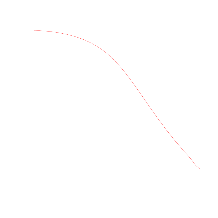
Figure 3: The ratio of the correction factors, $\chi_{ecc}/\chi_{st}$, for the eccentric and straight orbits of the satellite. The lines correspond to the orbits with eccentricities running from $e=0$ to 1 with a step of 0.1, in the Hernquist model for the galaxy. Here $\alpha\equiv a/R_{p}$, where $a$ is the scale length of the model and $R_{p}$ is the perigalacticon of the orbit. In the calculation of each curve, we assumed the same angular momentum of the straight orbit as for the corresponding eccentric orbit. Accordingly, the value of $\chi_{st}$ may vary for each line. Adiabatic corrections are not included. Had they been, the correction factors for $e\rightarrow 0$ would have been reduced dramatically.

Figure 3 shows the ratio $\chi_{ecc}/\chi_{st}$ for the orbits with various eccentricities. For highly eccentric orbits, $e\lesssim 1$, the ratio varies slightly with $\alpha$, from $\chi_{ecc}/\chi_{st}\approx 1.8$ for $\alpha\ll 1$ to $\chi_{ecc}/\chi_{st}=1$ for $\alpha\gg 1$. The latter limit corresponds to the most eccentric Keplerian orbit where both approaches must agree. However, as the eccentricity decreases, the ratio $\chi_{ecc}/\chi_{st}$ varies with $\alpha$ much more strongly. While at $\alpha\ll 1$, the ratio is highest for $e=0$, the opposite is true for $\alpha\gg 1$.

3.2 The power-law models

The power-law models are scale-free and allow further simplification of equations (30). We have $B_{i}(\alpha,e)\equiv\alpha^{n-2}\,C_{i}(e)$, $j^{2}(\alpha,e)\equiv\alpha^{n-4}\,f(e)$, and therefore

$$\langle\Delta E\rangle = {G\,M_{0}\over R_{max}^{3}}\,r^{2}\,\alpha^{n}\,\chi_{ecc}(e)\,A_{1}(x_{t}),$$ (34)

$$\chi_{ecc} \equiv {(C_{1}-C_{3})^{2}+(C_{2}-C_{3})^{2}+C_{3}^{2}\over 6f(e)}.$$ (35)

The remaining integrals depend only on the eccentricity $e$. After some algebra, we obtain

$$C_{1} = n\,\int_{-\theta_{m}}^{\theta_{m}}\,\left({R\over R_{p}}\right)^{2-n}\,\cos^{2}{\theta}\,d\theta,$$ (36a)

$$C_{2} = n\,\int_{-\theta_{m}}^{\theta_{m}}\,\left({R\over R_{p}}\right)^{2-n}\,\sin^{2}{\theta}\,d\theta,$$ (36b)

$$C_{3} = \int_{-\theta_{m}}^{\theta_{m}}\,\left({R\over R_{p}}\right)^{2-n}\,d\theta.$$ (36c)

Note that in the harmonic oscillator potential ($n=0$), the first two integrals are identically zero: $C_{1}=C_{2}=0$. The third one can be done using simple analytic orbits allowed in this potential (eq. [B2]):

$$C_{3}=\pi\,{1+e\over 1-e},\;\;\;\;\;\;\chi_{ecc}={\pi^{2}\over 2}\;\;\;\;(\mbox{for }n=0).$$ (37)

Surprisingly enough, the change of the stellar energy depends neither on the location in the galaxy, $\alpha$, nor on the orbital eccentricity, $e$. The satellite is equally compressed in all directions:

$$\Delta\mbox{\bf v} = \left({GM_{0}\over R_{max}^{3}}\right)^{1/2}\,\pi\,\{-x,-y,-z\},$$ (38)

$$\langle\Delta E\rangle = {GM_{0}\over R_{max}^{3}}\,{\pi^{2}\over 2}\,r^{2}\,A_{1}(x_{t})\;\;\;\;(\mbox{for }n=0).$$ (39)

In the isothermal sphere potential ($n=2$), the integrals are also done straightforwardly:

$$C_{1} = 2\theta_{m}+\sin{2\theta_{m}},$$ (40a)

$$C_{2} = 2\theta_{m}-\sin{2\theta_{m}},$$ (40b)

$$C_{3} = 2\theta_{m},\;\;\;\;\;\;(\mbox{for }n=2).$$ (40c)

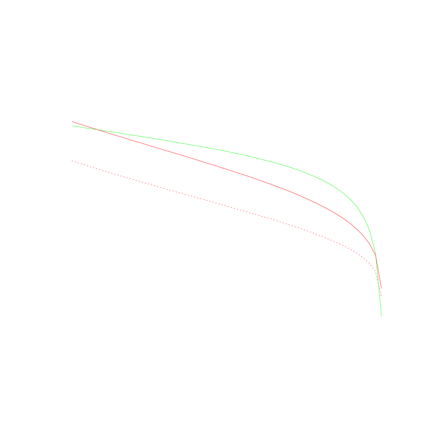
Figure 4: The correction factor $\chi_{ecc}$ for the power-law models (eq. [35]) versus the eccentricity of the orbit (solid lines). For the isothermal sphere ($n=2$), we also show the straight-path approximation, $\chi_{st}$ (dots).

For the $n=1$ model, the integrals $C_{i}(e)$ are done numerically. Figure 4 shows the factors $\chi_{ecc}$ for all three models. For comparison, we also plot $\chi_{st}$ for the isothermal sphere model. Heating on eccentric orbits is larger than that on the straight path, except for $e=1$, where the two are equal. However, the plot does not include adiabatic corrections, which would have effectively reduced heating on low-eccentricity orbits.

4 A Case Study: NGC 6712

We now illustrate the theory developed in §3 by considering the evolution of a globular star cluster, NGC 6712. This cluster is presently at the distance of 3.8 kpc from the Galactic center, close enough to experience tidal shocking by the Galactic bulge. We use the observed parameters to construct cluster’s orbit in the bulge potential and to integrate the expected energy change. Then, we perform N-body simulations to verify the result. Finally, we consider various orbital eccentricities allowed by the cluster orbital energy and illustrate the eccentricity effect on the resulting heating.

4.1 Constructing the orbit

Full three-dimensional kinematic data for NGC 6712 are not yet available. Instead, we use the results of Monte-Carlo simulations by Gnedin & Ostriker (1997) for the Ostriker-Caldwell (1983) model of the Galaxy with the isotropic velocity distribution of the globular cluster system. We draw the two unknown components of the orbital velocity consistent with the chosen kinematic model and integrate the orbits for $10^{10}$ yr. For NGC 6712, the median perigalactic distance is $R_{p}=0.73$ kpc and the velocity at perigalacticon is $V_{p}=396$ km s^-1. The eccentricity of this orbit is $e=0.69$.

We approximate the Galactic bulge by a Hernquist model with the scale-length $a=0.6$ kpc. The total mass of the model required to reproduce the observed velocity $V_{p}$ is $M_{0}=3.3\times 10^{10}\,M_{\sun}$, close to the observed mass of the bulge.

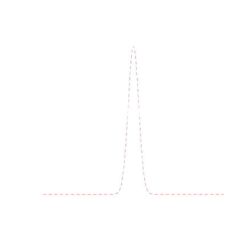
Figure 5: Time variation of the vertical component of the tidal force exerted on globular cluster NGC 6712 by the Galactic bulge. Solid line is the actual force, whereas dashes show the Gaussian fit with the effective width $\tau=5.3\,t_{dyn}$. The force is in units of the N-body code.

Figure 5 shows the vertical component of the tidal force exerted on the cluster along a single orbit in the Galaxy. The force peaks at the perigalacticon. The dashed line shows that the Gaussian fit to the actual force, $F_{fit}\propto e^{-t^{2}/\tau^{2}}$, is accurate for the most important part of the orbit. (A similar parameterization was employed by Johnston, Hernquist & Weinberg (1998) in their numerical study of tidal heating.) The width of the Gaussian, or the effective duration of the shock, is $\tau\approx 5.3\,t_{dyn}$, where $t_{dyn}$ is the half-mass dynamical time of the cluster. This timescale is long enough that most stars in the cluster are protected by adiabatic invariants, even for $R_{p}<1$ kpc. Using the calculated value of $\tau$, we estimate adiabatic corrections to the energy change (cf. eq. [33]) and verify them with N-body simulations described next.

4.2 Self-Consistent N-body simulations

We can now simulate the cluster as a system of $N$ point-mass particles and run it along the chosen orbit. At the end, we calculate the changes of the stellar energies and compare them with our analytic theory.

We use a Self-Consistent Field code (Hernquist & Ostriker (1992), Gnedin & Ostriker 1998) with $N=10^{6}$ particles. The code approximates the true gravitational potential and density of the cluster with a finite series of basis functions. In this work, we take $n=10$ radial functions and $l=6$ spherical harmonics.

The initial cluster realization is a King model with the concentration parameter $c=0.84$. It is sufficiently close to the observed concentration of NGC 6712, $c\approx 0.9$. The code employs units in which $G=1$, $M_{cl}=1$, and $R_{c}=1$, where $M_{cl}$ and $R_{c}$ are the mass and the initial core radius of the cluster. The physical units are fixed by the observed values, $M_{cl}=2.5\times 10^{5}\,M_{\sun}$ and $R_{c}=1.9$ pc.

In this simulation, the gravitational potential of the cluster is kept fixed. The self-consistent response of the system to tidal perturbations is studied elsewhere (Gnedin & Ostriker 1998) and is not important for our discussion. We run the cluster along the orbit, starting from the apogalacticon, where the tidal force is minimal (cf. Figure 5), going to the perigalacticon, and then moving to the next apogalacticon. The whole simulation lasts for about 200 dynamical times, $t_{dyn}$, of the cluster, with a short enough time step to ensure accurate integration of stellar orbits; $\Delta t=0.01\,t_{dyn}$. We have run the simulation on the SGI Origin 2000 supercomputer at the Princeton University Observatory.

Figure 6 shows the first and second order energy changes at the end of the simulation. The particles are grouped in equal size bins, ranked by their initial energy, and the mean values, $\langle\Delta E\rangle$ and $\langle\Delta E^{2}\rangle$, and their standard errors are calculated for each bin. The data are compared with our analytic result (eqs. [31,32]), wherein adiabatic corrections (eq. [33] with $\gamma_{1}=1.4$, $\gamma_{2}=1.5$) are appropriate for the long duration of the shock, $\tau$, estimated in §4.1. Had we used the simplest theory, presented in §2, for straight line orbits without adabatic corrections, we would have overestimated the total energy change significantly. By calculating the correct orbits and employing adiabatic corrections, we find a very good agreement with the simulations. This excellent agreement encourages one to use the semi-analytical theory (eqs. [31-33]) to study the effects of tidal shocks on the evolution of star clusters and satellite galaxies.

4.3 Effects of orbital eccentricity

Finally, we demonstrate how the eccentricity of the orbit affects the resulting heating. We keep the orbital energy of NGC 6712 fixed and consider all allowed eccentricities. Since these two parameters ($E_{orb}$ and $e$) specify the orbit, the perigalactic distance $R_{p}$ varies accordingly with $e$. Increasing eccentricity decreases $R_{p}$ and vice versa. Also, low eccentricity orbits have longer shock durations, $\tau$, which leads to significant adiabatic corrections.

Figure 7 shows the energy change at the half-mass radius of the cluster, calculated from equations (31,33). The value of $\langle\Delta E\rangle_{h}$ falls dramatically with decreasing eccentricity, in part because $R_{p}$ increases as $e$ decreases and largely because of the adiabatic corrections. As expected, there is essentially no heating on nearly circular orbits. Also, we calculate the median energy change, $\langle\Delta E\rangle_{h}$, for two more cases, when the orbital energy is a half and twice the observed value. The more bound orbits tend to have a shorter timescale $\tau$ and correspondingly larger energy input than the less bound orbits.

5 Discussion

Our analysis applies to weak gravitational perturbations, tidal shocks. A significant evolution of a satellite or a star cluster occurs over a number of successive shocks. In this respect, the current work differs from that of Aguilar & White (1985,1986) who studied the effects of strong interactions between two similar mass galaxies. Their work showed that the impulsive approximation is adequate for the most regions where a significant mass loss and energy changes occur.

Aguilar & White emphasized that particles escaping the satellite after the perturbation should be excluded from the analysis of the remaining structure. In the case of tidal shocks, few stars leave the satellite immediately. Instead, they slowly drift in the energy space (see Figure 6) and eventually escape through the tidal boundary.

The results of our calculations are useful for semi-analytical studies of tidal interactions between large galaxies and their dwarf companions or star clusters. For example, Gnedin & Ostriker (1997) estimated the amount of heating of globular clusters due to the Galactic bulge by inserting equations (11, 13, 14) into their Fokker-Planck code. Assuming the spherical symmetry of the cluster, the code solves the Fokker-Planck equation for the distribution function of stars in energy space. Since the amplitude of perturbations is small, the first two terms of the expansion of the Master equation (for example, van Kampen (1981); Gardiner (1985)) are both linear in the perturbation energy and lead to the Fokker-Planck formulation. The higher order terms are negligible and can be ignored. This approach is much faster than a full N-body simulation and allows a direct comparison with analytical models of star clusters. A new detailed study of the globular cluster evolution including tidal shocks is presented in Gnedin, Lee, & Ostriker (1998).

6 Summary

We have calculated the tidal field of a spherical mass distribution. Using the impulse approximation, coupled with adiabatic corrections, we estimated the amount of heating of stars in the satellite during a tidal shock. We considered several mass distributions for the host galaxy, a Hernquist model and three power-law profiles, and explored various satellite orbits. Although we restricted ourselves to spherically-symmetric galaxies to simplify the analysis, our results should also hold for non-spherical systems with a modest amount of flattening.

For the Hernquist model, we found that heating is enhanced by a factor of few on eccentric orbits compared to the conventional straight path approximation. However, adiabatic corrections prevent any heating on low-eccentricity orbits. In the harmonic oscillator potential, the satellite is equally compressed in all directions. In the isothermal sphere potential, heating on eccentric orbits is also larger than that in the straight path approximation.

To illustrate the analytic results (eqs. [31-33]), we considered the example of globular cluster NGC 6712. For a fixed orbital energy of the cluster, the heating is much larger on highly eccentric orbits than on low-eccentricity orbits because of the adiabatic corrections. N-body simulations confirm the validity of our method, which becomes a powerful tool in calculating the tidal heating of satellites of larger galaxies. This semi-analytic method can also be used for studying the evolution of giant star clusters in galactic nuclei or the disruption of dwarf satellites in groups of galaxies.

Appendix A Calculation of the tidal integrals for the Hernquist model

We evaluate here the tidal integrals (eq. [11]) for the Hernquist model. The normalized mass profile is given by equation (19). Denoting $\alpha\equiv a/R_{p}$, the first integral is

$$I_{0}(\alpha)=\int_{1}^{\infty}{\zeta^{2}\over(\zeta+\alpha)^{2}}\,{d\zeta\over\zeta^{2}(\zeta^{2}-1)^{1/2}}.$$ (A1)

Substituting $x=(\zeta+\alpha)^{-1}$, we have

$$I_{0}(\alpha)=\int_{0}^{(1+\alpha)^{-1}}{x\,dx\over[1-2\alpha x+(\alpha^{2}-1)x^{2}]^{1/2}}.$$ (A2)

Now for $\alpha>1$, we take $y=\alpha-(\alpha^{2}-1)x$, and

$$I_{0}(\alpha)=(\alpha^{2}-1)^{-3/2}\int_{1}^{\alpha}{(\alpha-y)dy\over(y^{2}-1)^{1/2}}=-\frac{1}{\alpha^{2}-1}+{\alpha\over(\alpha^{2}-1)^{3/2}}\ln{(\alpha+(\alpha^{2}-1)^{1/2})}.$$ (A3)

For $\alpha<1$, we have $y=\alpha+(1-\alpha^{2})x$:

$$I_{0}(\alpha)=(1-\alpha^{2})^{-3/2}\int_{\alpha}^{1}{(y-\alpha)dy\over(1-y^{2})^{1/2}}=\frac{1}{1-\alpha^{2}}-{\alpha\over(1-\alpha^{2})^{3/2}}\arccos{\alpha}.$$ (A4)

It is straightforward to verify that both expressions match smoothly at $\alpha=1$; $I_{0}(1)=\text@frac{1}{3}$. The next integral, $J_{0}(\alpha)$, can be reduced to the already calculated $I_{0}$. Taking $x=\zeta^{-1}$, we get

$$J_{0}(\alpha) = \int_{0}^{1}{x^{3}dx\over(1+\alpha x)^{2}(1-x^{2})^{1/2}}=\frac{1}{\alpha^{2}}\int_{0}^{1}{(\alpha^{2}x^{2}+2\alpha x+1-1-2\alpha x)xdx\over(1+\alpha x)^{2}(1-x^{2})^{1/2}}$$ (A5)

$$= {1-I_{0}\over\alpha^{2}}-{2\over\alpha}\int_{0}^{1}{x^{2}dx\over(1+\alpha x)^{2}(1-x^{2})^{1/2}}$$

$$= {1+3I_{0}\over\alpha^{2}}-{\pi\over\alpha^{3}}-{2I_{0}\over\alpha^{4}}+{2\over\alpha^{4}}\int_{0}^{1}{(\alpha+x)dx\over(1+\alpha x)^{2}(1-x^{2})^{1/2}}.$$

Now it is useful to note that

$$\int_{0}^{1}{(\alpha+x)dx\over(1+\alpha x)^{2}(1-x^{2})^{1/2}}\equiv 1$$ (A6)

for all values of $\alpha$. Thus, we arrive at

$$J_{0}(\alpha)={\alpha^{2}-\pi\alpha+2+(3\alpha^{2}-2)I_{0}(\alpha)\over\alpha^{4}}.$$ (A7)

The remaining two integrals are easily calculated using the identity (12), or

$$I_{1}(\alpha)=-\alpha{dI_{0}(\alpha)\over d\alpha},\hskip 28.45274ptJ_{1}(\alpha)=-\alpha{dJ_{0}(\alpha)\over d\alpha}.$$ (A8)

For convenience, all four integrals are combined below.

$$I_{0}=\left\{\begin{array}[]{lr}\frac{1}{1-\alpha^{2}}-\frac{\alpha}{(1-\alpha^{2})^{3/2}}\,\arccos{\alpha},&[\alpha<1]\\ \\ \frac{1}{3}\approx 0.33333,&[\alpha=1]\\ \\ \frac{1}{1-\alpha^{2}}+\frac{\alpha}{(\alpha^{2}-1)^{3/2}}\,\ln(\alpha+(\alpha^{2}-1)^{1/2}),&[\alpha>1]\end{array}\right.$$ (A9a)

$$I_{1}=\left\{\begin{array}[]{lr}-{3\alpha^{2}\over\left(1-\alpha^{2}\right)^{2}}+\frac{\alpha(1+2\alpha^{2})}{(1-\alpha^{2})^{5/2}}\,\arccos{\alpha},&[\alpha<1]\\ \\ \frac{4}{15}\approx 0.26667,&[\alpha=1]\\ \\ -\frac{3\alpha^{2}}{(\alpha^{2}-1)^{2}}+\frac{\alpha(1+2\alpha^{2})}{(\alpha^{2}-1)^{5/2}}\,\ln(\alpha+(\alpha^{2}-1)^{1/2}),&[\alpha>1]\end{array}\right.$$ (A9b)

$$J_{0}=\left\{\begin{array}[]{lr}{-\alpha^{3}+\pi\alpha^{2}+2\alpha-\pi\over\alpha^{3}\left(1-\alpha^{2}\right)}-{3\alpha^{2}-2\over\alpha^{3}\left(1-\alpha^{2}\right)^{3/2}}\,\arccos{\alpha},&[\alpha<1]\\ \\ {10\over 3}-\pi\approx 0.19174,&[\alpha=1]\\ \\ {-\alpha^{3}+\pi\alpha^{2}+2\alpha-\pi\over\alpha^{3}\left(1-\alpha^{2}\right)}+{3\alpha^{2}-2\over\alpha^{3}\left(\alpha^{2}-1\right)^{3/2}}\,\ln(\alpha+(\alpha^{2}-1)^{1/2}),&[\alpha>1]\end{array}\right.$$ (A9c)

$$J_{1}=\left\{\begin{array}[]{lr}{2\alpha^{5}-3\pi\alpha^{4}-11\alpha^{3}+6\pi\alpha^{2}+6\alpha-3\pi\over\alpha^{3}\left(1-\alpha^{2}\right)^{2}}+{12\alpha^{4}-15\alpha^{2}+6\over\alpha^{3}\left(1-\alpha^{2}\right)^{5/2}}\,\arccos{\alpha},&[\alpha<1]\\ \\ 9.6-3\pi\approx 0.17522,&[\alpha=1]\\ \\ {2\alpha^{5}-3\pi\alpha^{4}-11\alpha^{3}+6\pi\alpha^{2}+6\alpha-3\pi\over\alpha^{3}\left(\alpha^{2}-1\right)^{2}}+{12\alpha^{4}-15\alpha^{2}+6\over\alpha^{3}\left(\alpha^{2}-1\right)^{5/2}}\,\ln(\alpha+(\alpha^{2}-1)^{1/2}),&[\alpha>1]\end{array}\right.$$ (A9d)

Appendix B Orbit integration

We describe here an accurate procedure to calculate orbits in a given potential. The four dimensionless potentials used in this paper and the corresponding angular momenta are given in Table B. The angular momentum of an orbit of the given perigalactic distance and eccentricity is found by equating the orbital energy at the perigalacticon and the apogalacticon.

We integrate the orbits using the following quadratures:

$$\theta = \int_{r_{p}}^{r}\,{dr\over r^{2}\left({2\varepsilon-2\phi(r)\over j^{2}}-{1\over r^{2}}\right)^{1/2}}$$ (B1a)

$$t = \int_{r_{p}}^{r}\,{dr\over j\left({2\varepsilon-2\phi(r)\over j^{2}}-{1\over r^{2}}\right)^{1/2}},$$ (B1b)

where $r$ is the dimensionless radius, $r\equiv R/a$ or $r\equiv R/R_{max}$, and $\varepsilon$ is the dimensionless energy of the orbit. To avoid singularities at both the perigalacticon and the apogalacticon, we separate the integrals into two parts at some intermediate radius, $r_{div}\equiv(1+e)r_{p}$. Then, we change the variables of integration individually for the two parts to remove singularities. For $r_{p}\leq r\leq r_{div}$, the new variable is $u_{1}\equiv\sqrt{\alpha-{1\over r}}$; for $r_{div}\leq r\leq r_{a}$, it is $u_{2}\equiv\sqrt{{1\over r}-\alpha{1-e\over 1+e}}$. Both parts of the integrals are regular in $u_{1}$ or $u_{2}$ and can be calculated numerically with high accuracy.

Note, that in the harmonic oscillator potential the orbits allow simple analytic solution. In Cartesian coordinates,

$$x=r_{p}\,\cos{t},\;\;\;\;\;\;y=r_{a}\,\sin{t},$$ (B2)

where

$$t=\arctan{\left({1-e\over 1+e}\,\tan{\theta}\right)}.$$ (B3)

Model	Potential, $\phi(r)$	Angular momentum, $j^{2}(\alpha,e)$
Hernquist model	$-{1\over 1+r}$	${(1+e)^{2}\over\alpha(1+\alpha)(1+\alpha+(1-\alpha)e)}$
Harmonic oscillator	${r^{2}\over 2}-{3\over 2}$	$\alpha^{-4}\,{(1+e)^{2}\over(1-e)^{2}}$
Power-law, $n=1$	$r-2$	$\alpha^{-3}\,{(1+e)^{2}\over 1-e}$
Singular isothermal sphere	$\ln{r}-1$	$\alpha^{-2}\,{(1+e)^{2}\over 2e}\,\ln{1+e\over 1-e}$

Figure 1: Integrals $I_{0}$, $J_{0}$, $I_{1}$, and $J_{1}$ (eq. [A9d]) for the Hernquist model.

Figure 2: Corrections to the velocity change relative to the point-mass approximation for the Hernquist model (cf eq. [20]). The value of $\chi_{y}$ is always close to zero, as it would be in a point-mass potential. For comparison, dashes show the fraction of the galactic mass inside the perigalacticon, $\chi_{0}=\mbox{$\mu$}(R_{p})$.

Figure 6: The first and second order energy changes for globular cluster NGC 6712 (triangles). Both changes are plotted versus the initial energy of stars, $E_{i}$, and are normalized to the corresponding power of $E_{i}$. Error-bars indicate standard deviations in each energy bin. Here $E_{bind}$ is the initial binding energy of the system, and arrows are at the core and the half-mass radii. Solid lines are the analytic predictions (eq. [31]).

Figure 7: Energy change of stars at the half-mass radius of NGC 6712 relative to the initial half-mass energy as a function of eccentricity of the orbit, $e$, and the corresponding perigalactic distance, $R_{p}$. The orbital energy is fixed at the observed value for the cluster (solid line) or at one-half and twice that value (dashed lines below and above the solid line, respectively). The star marks the eccentricity of NGC 6712 in our kinematic model (see §4.1). For illustration, we also show on the right-hand-side axis the approximate destruction time of the cluster due only to tidal shocks. The destruction time is defined as $t_{destr}\equiv P_{orb}(E_{h}/\Delta E_{h})$, where $P_{orb}$ is the cluster orbital period, which varies with eccentricity. In contrast to Figure 3, which did not allow for adiabatic corrections, here tidal shocking vanishes as $e\rightarrow 0$.

References

- (1) Aguilar, L. A., & White, S. D. M. 1985, ApJ, 295, 374
- (2) Aguilar, L. A., & White, S. D. M. 1986, ApJ, 307, 97
- (3) Binney, J., & Tremaine, S. 1987, Galactic Dynamics (Princeton: Princeton Univ. Press)
- Gardiner (1985) Gardiner, C. W. 1985, Handbook of stochastic processes (Berlin: Springer-Verlag)
- Gnedin, Lee, & Ostriker (1998) Gnedin, O. Y., Lee, H. M., & Ostriker, J. P. 1998, ApJ, submitted; astro-ph/9806245
- Gnedin & Ostriker (1997) Gnedin, O. Y., & Ostriker, J. P. 1997, ApJ, 474, 223
- (7) Gnedin, O. Y., & Ostriker, J. P. 1998, ApJ, submitted
- Hernquist (1990) Hernquist, L. 1990, ApJ, 356, 359
- Hernquist & Ostriker (1992) Hernquist, L., & Ostriker, J. P. 1992, ApJ, 386, 375
- Johnston, Hernquist & Weinberg (1998) Johnston, K.V., Hernquist, L., & Weinberg, M.D. 1998, ApJ, submitted
- Johnston et al. (1995) Johnston, K.V., Spergel, D. N., & Hernquist, L. 1995, ApJ, 451, 598
- Knobloch (1976) Knobloch, E. 1976, ApJ, 209, 411
- Kroupa (1997) Kroupa, P. 1997, New Astronomy, 2, 139
- (14) Murali, C., & Weinberg, M. D. 1997a, MNRAS, 288, 749
- (15) Murali, C., & Weinberg, M. D. 1997b, MNRAS, 288, 767
- (16) Murali, C., & Weinberg, M. D. 1997c, MNRAS, 291, 717
- Oh & Lin (1992) Oh, K. S., & Lin, D. N. C. 1992, ApJ, 386, 519
- Oh, Lin & Aarseth (1992) Oh, K. S., Lin, D. N. C., & Aarseth, S. J. 1992, ApJ, 386, 506
- Oh, Lin & Aarseth (1995) Oh, K. S., Lin, D. N. C., & Aarseth, S. J. 1995, ApJ, 442, 142
- Ostriker & Caldwell (1983) Ostriker, J. P., & Caldwell, J. A. 1983, in Kinematics, Dynamics and Structure of the Milky Way, ed. W. L. H. Shuter (Dordrecht: Reidel), 249
- Richstone (1975) Richstone, D. 1975, ApJ, 200, 535
- Spitzer (1958) Spitzer, L. Jr. 1958, ApJ, 127, 17
- Spitzer (1987) Spitzer, L. Jr. 1987, Dynamical Evolution of Globular Clusters (Princeton: Princeton Univ. Press)
- van Kampen (1981) van Kampen, N. G. 1981, Stochastic processes in physics and chemistry (Amsterdam: North-Holland)
- (25) Weinberg, M. D. 1994a, AJ, 108, 1398
- (26) Weinberg, M. D. 1994b, AJ, 108, 1403
- (27) Weinberg, M. D. 1994c, AJ, 108, 1414
- Weinberg (1997) Weinberg, M. D. 1997, ApJ, 478, 435