Evolution of the Lyman$\alpha$ forest from high to low redshift

Abstract

We study the evolution with redshift, from $z\sim 5$ to $z=0$, of the Lyman$\alpha$ forest in a CDM model using numerical simulations including collisionless particles only. The baryonic component is assumed to follow the dark matter distribution.

We distinguish between two populations of particles: Population $P_{\rm s}$ traces the filamentary structures of the dark matter, evolves slowly with redshift and, for $N(\mbox{H{\sc i}})\ga 10^{14}\mbox{ cm${}^{-2}$}$, dominates the number density of lines at $z<3$; most of population $P_{\rm u}$ is located in underdense regions and for the same column densities, disappears rapidly at high redshift.

We generate synthetic spectra from the simulation and show that the redshift evolution of the Lyman$\alpha$ forest (decrement, $N(\mbox{H{\sc i}})$ distribution) is well reproduced over the whole redshift range for $\Omega_{\rm b}h^{2}\sim 0.0125$ and $J_{-21}\approx 0.1$ at $z\sim 3$ where $J_{-21}$ is the UV background flux intensity in units of $10^{-21}$ erg cm^-2 s^-1 Hz^-1 sr^-1.

The total number of lines with $N(\mbox{H{\sc i}})\ga 10^{12}\mbox{ cm${}^{-2}$}$ remains approximately constant from $z\sim 4$ to $z=1$. At $z\sim 0$, the number density of lines per unit redshift with $\log N(\mbox{H{\sc i}})>12,13,14$ is of the order of 400, 100, and 20 respectively. Therefore, at low redshift, if most of the strong ($w_{\rm r}>0.3\mbox{ \AA}$) lines are expected to be associated with galaxies, the bulk of the Lyman$\alpha$ forest however should have lower equivalent width and should not be tightly correlated with galaxies.

1 Introduction

Recent high spectral resolution and high ${\rm S}/{\rm N}$ ratio observations of the Lyman$\alpha$ forest have shed some light on previous discussions about the physical properties of the gas.

There is a cut-off in the Doppler parameter distribution with only a very small fraction of narrow lines ($b<15\mbox{ km s${}^{-1}$}$) which cannot be identified with metal-lines (Rauch et al. 1992). The large $b$ values could reflect blending of several components with similar properties (Hu et al. 1995), in which case the gas would have a quite homogeneous temperature ($T\approx 24\,000\mbox{ K}$), and turbulent motions inside one cloud would be small. The Hi column density distribution is well fitted by a power-law ${\rm d}n/{\rm d}N\propto N^{-\beta}$ with $\beta\approx 1.5$ in the range $13.5<\log N(\mbox{H{\sc i}})<15.5$ (Hu et al. 1995, Lu et al. 1996). For $\log N(\mbox{H{\sc i}})\ga 15$, there is a deficit of lines (Petitjean et al. 1993), compared to the power-law function. The amplitude of the deficit seems to evolve with redshift, being larger at $z\sim 2.5$ than at $z\sim 3.5$ (Kim et al. 1997).

For $\log N(\mbox{H{\sc i}})<13.5$, blending effects depress the observed distribution. Synthetic spectra generated from a random realisation out of an artificial population of clouds show that the underlying column density distribution has no turn over at low column density. The correction however can be very large. At $\log N(\mbox{H{\sc i}})\approx 12.4$, 6% of the lines are recovered at $z\sim 3.7$ (Lu et al. 1996, Kim et al. 1997). The way the correction is done may not be the unique solution. In particular, if the Lyman$\alpha$ complexes have large dimensions, the redshift range corresponding to the Hubble flow and velocity structure of the cloud along the radial dimension must be avoided. The large dimensions ($100-300\mbox{ kpc}$, Dinshaw et al. 1995, Smette et al. 1995, Crotts & Fang 1997) recently derived from observations of lines of sight towards quasars projected on the sky at small separations may support this remark. The existence of a turn-over in the column density is thus still a matter of debate; the question being related to the effective size of the complexes. More data are needed to investigate this question.

One of the most important issue to clarify towards understanding nature of the Lyman$\alpha$ forest is the relation between the Lyman$\alpha$ forest and galaxies. Although conclusions are uncertain, it seems that at least the strongest lines in the Lyman$\alpha$ forest at low redshift are anyhow associated with galaxies (Lanzetta et al. 1995, Le Brun et al. 1996). This is not really surprizing since if there is gas in the intergalactic medium (and it seems there is), we can expect the density of this gas to be higher in the vicinity of the galactic potential wells. The case for the weak lines to be associated with galaxies is less clear. Indeed observations of the line of sight to 3C273 that are the most sensitive to the presence of weak lines (Morris et al. 1991, Bahcall et al. 1991) indicate the presence of a large number of these lines and no clear association with galaxies is seen (Morris et al. 1993, see also Bowen et al. 1997). In addition, using a high ${\rm S}/{\rm N}$ ratio spectrum of H1821+643 ($z_{\rm em}=0.297$), Tripp et al. (1997) have found that, the number per unit redshift of lines with $w_{\rm r}>50\mbox{ m\AA}$ is $112\pm 21$. Moreover, Stocke et al. (1995) have detected weak absorption lines located in regions devoided of galaxies.

Recent observations have shown that at redshift $z\sim 3$, Civ is found in 90% of the clouds with $N(\mbox{H{\sc i}})>10^{15}\mbox{ cm${}^{-2}$}$ and in about 50% of the clouds with $3\times 10^{14}\mbox{ cm${}^{-2}$}<N(\mbox{H{\sc i}})<10^{15}\mbox{ cm${}^{-2}$}$ (Songaila & Cowie 1996, Cowie et al. 1995). Several components are seen in most of these weak systems; thus the two-point correlation function shows a signal on scale smaller than $200\mbox{ km s${}^{-1}$}$. On this basis, Fernández-Soto et al. (1996) show that the observed clustering is broadly compatible with that expected for galaxies. It can be argued however that the signal detected in the correlation function is not related to clustering of galaxies but instead reflects the velocity structure of the Lyman$\alpha$ gas inside large complexes. Although such clustering is observed as well for metal line systems (Petitjean & Bergeron 1994, see Cristiani et al. 1996), this does not mean that both Lyman$\alpha$ complexes and metal line systems are identical in nature since Lyman$\alpha$ complexes have lower abundances (Hellsten et al. 1997) and larger dimensions.

Indeed a more attractive picture arises from simulations showing that the Lyman$\alpha$ absorption line properties can be understood if the gas traces the gravitational potential of the dark matter (Cen et al. 1994, Petitjean et al. 1995, Mücket et al. 1996, Hernquist et al. 1996, Miralda-Escudé et al. 1996, Zhang et al. 1996, Bi & Davidsen 1996). In this picture, part of the gas is located inside filaments where star formation can occur very early in small halos that subsequently merge to build-up a galaxy (Haehnelt et al. 1996). It is thus not surprizing to observe metal lines from this gas. The remaining part of the gas either is loosely associated with the filaments and has $N(\mbox{H{\sc i}})\ga 10^{14}\mbox{ cm${}^{-2}$}$ or is located in the underdense regions and has $N(\mbox{H{\sc i}})\la 10^{14}\mbox{ cm${}^{-2}$}$. Most of the Lyman$\alpha$ forest arises in this gas and it is still to be demonstrated that it contains metals.

To clarify these issues, it is important to follow the evolution of the Lyman$\alpha$ gas over a wide redshift interval up to the current epoch ($z=0$) distinguishing between gas closely associated with the filamentary structures of the dark matter and the dilute gas mainly located in the underdense regions. The problem which the true hydrodynamic simulations are still confronted with is the huge amount of computer time needed to model a whole line of sight. The goal of our paper is then twofold: to investigate the time-dependence of the Lyman$\alpha$ forest along the whole line of sight, and to investigate the relative contributions of the two different gas distributions to the forest characteristics. In Section 2. we discuss the main assumptions of the model and the limits of applicability. Results and predictions of the model are presented in Section 3. and conclusions are drawn in Section 4.

2 Model and simulations

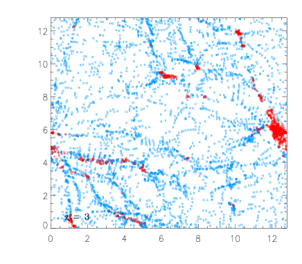
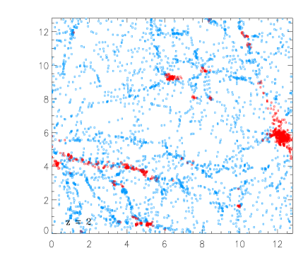
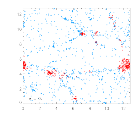
Figure 1: “Unshocked” (open squares) and “shocked” (filled squares) clouds in a slice of 50 kpc thickness of a simulation (12.8 Mpc)³ box at different redshifts: $z=3$ (top), $z=2$ (middle), $z=0$ (bottom); the size of the symbols is comparable to the resolution.

We have used the particle-mesh code described in detail by Kates et al. (1991), modified as described in our previous paper (Mücket et al. 1996). A particle simulation is used in order to investigate the evolution of the Lyman$\alpha$ forest over a wide redshift range using two main assumptions:

First, the Lyman$\alpha$ gas traces the shallower potential wells of the dark matter distribution. In previous papers (Petitjean et al. 1995, Mücket et al. 1996) we have already discussed in detail the applicability of this approximation as well as its consequences: the gas with column density smaller than $10^{17}\mbox{ cm${}^{-2}$}$ closely follows the dark matter distribution. This assumption has been shown to be valid for the low-density regime characteristic of the Lyman$\alpha$ forest by detailed hydro-simulations (see Miralda-Escudé et al. 1996, Hernquist et al. 1996, Yepes et al. 1997, and also Gnedin et al. 1997, Hui et al. 1997).

Secondly, a procedure to determine the gas temperature has to be introduced. We follow Kates et al. (1991) where it is assumed that energy is acquired by the gas, in addition to photo-ionization, when shell crossing takes place in the dark matter dynamics. Particles that have acquired this way enough energy to increase the temperature above $T>T_{\rm th}=20\,000\mbox{ K}$ are called ’shocked’ (Population $P_{\rm s}$). This temperature corresponds to the lower limit of the range of equilibrium temperatures found for different densities and UV flux intensities in highly ionized metal-poor gas. Other particles are called ’unshocked’ (Population $P_{\rm u}$). The thermal history is followed as described in Mücket et al. (1996) taking into account adiabatic effects, radiative cooling processes, Compton cooling and heating. As discussed in the previous paper, this is a reasonable treatment as far as the Lyman$\alpha$ forest is concerned. Clearly our approximation fails for column densities $N(\mbox{H{\sc i}})>10^{17}\mbox{ cm${}^{-2}$}$. Therefore a description of the distribution and state of the gas in dense collapsing regions would lead to uncertain results.

To first order, the distinction between ’shocked’ and ’unshocked’ gas in the code is independent of resolution since shocks should be supressed by thermal pressure in population $P_{\rm u}$. The approximation is valid if the grid size is smaller than the Jeans length. According to Mücket et al. (1996), this requires $2l_{\rm c}\leq 1.2\cdot(T_{4}/(1+z_{i}))^{1/2}\mbox{ Mpc}$ where $l_{\rm c}$ denotes the comoving length of a cell. At $z=5$ we obtain $l_{\rm c}\approx 240\mbox{ Mpc}$ which is fairly well realized in our simulations. The gas constituent of each particle can thus be considered as a non-collapsing diffuse gas element.

The gas is considered in thermal equilibrium. The assumption is no longer valid at very low densities. Our simulation is limited to the cosmic background density however and thus to $N(\mbox{H{\sc i}})>10^{12}\mbox{ cm${}^{-2}$}$ where deviation from equilibrium is minimized.

The simulations use $128^{3}$ particles on a $256^{3}$ grid and were carried out using a box size of 12.8 Mpc, which corresponds to a co-moving cell size of 50 kpc. The baryonic mass is assumed to be proportional to the dark matter mass inside a cell. We adopt a value for the Hubble parameter $H_{0}=50\mbox{ km Mpc${}^{-1}$ s${}^{-1}$}$ and $\Omega_{\rm b}=0.05$ throughout.

The intensity of the photo-ionizing UV background flux, assumed to be homogeneous and isotropic inside the simulation box, is computed in the course of the simulation. The ionizing spectrum is modeled as $J_{\nu}\propto J_{0}\,\nu^{-1}$ where $J_{0}=f(z)=J_{-21}\cdot 10^{-21}\mbox{ erg cm${}^{-2}$ s${}^{-1}$ Hz${}^{-1}$ sr${}^{-1}$}$ is the ionizing flux at 13.6 eV. The variation of the flux intensity with redshift $z$ is related both to the rate $\Delta m(T_{4}<0.5;z)$ at which the baryonic material cools below $T_{4}=0.5$ (with $T=T_{4}\cdot 10^{4}\mbox{ K}$) in the simulation and to the expansion of the Universe:

$$f(z) = C_{\rm cool}\,\Delta m(T_{4}<0.5;z)$$ (1)

$${}+f(z+\Delta z)\left(\frac{1+z}{1+z+\Delta z}\right)^{4},$$

where $C_{\rm cool}$ is a factor of proportionality. To avoid overcooling (e.g. Blanchard et al. 1992), we assume that the cool gas is transformed into stars with an efficiency $\varepsilon$ of about 8%. The remainder of the gas is reheated to temperatures above 50 000 K. The characteristic time scale for such processes is of order $t_{\ast}\approx 10^{8}\mbox{ years}$. This procedure provides therefore results that are independent of the time step. Whereas the time dependence of the UV flux is almost not affected by the value of $t_{\ast}$ within a reasonable range, the value of the efficiency parameter $\varepsilon$ has considerable influence on the flux intensity at small redshifts (see also Miralda-Escudé et al. 1996): in this scenario it determines the amount of gas still available at any time for star formation.

The dynamics of structure formation is highly sensitive to the initial fluctuation spectrum. Since we are working here on scales mainly determined by the $k^{-3}$ tail of the CDM spectrum, only the effective amplitude of the spectrum within the $k$-range of interest is of importance. In particular it affects the redshift evolution of the computed UV flux intensity. We have used this dependence to constrain the power of the initial density fluctuations in the simulation in order to be able to reproduce the observed evolution (see Section 3.2). The resulting effective power is 10% larger than what is expected from a COBE spectrum normalized at large scales.

During the simulation we distinguish between the two different populations of clouds defined above namely: population $P_{\rm s}$ corresponds to particles for which shock-heating has been important at some time of the thermal history of the particle and population $P_{\rm u}$ to particles for which photo-ionization is the dominant heating process all the time. Population $P_{\rm s}$ particles are mostly found in big halos and elongated filamentary structures (regions of enhanced density). The remainder of the gas (population $P_{\rm u}$) is present in the surroundings of the structures formed by shocked particles but mostly in the voids delineated by these structures.

The spatial distribution of both populations of particles at different redshifts ($z=3,2\mbox{, and }0$) in a slice of dimensions $12.8\times 12.8\times 0.05\mbox{ Mpc${}^{3}$}$ (comoving) is illustrated in Fig. 1. In this figure all particles in the slice are shown regardless of their neutral hydrogen content. The fraction of particles belonging to population $P_{\rm u}$ is changing with time: 77% at $z=3$, 67% at $z=2$, 40% at $z=0.5$ and 25% at $z=0$.

3 Results

3.1 Synthetic spectra

The modeling of the cloud distribution along a full line of sight up to a fictitious QSO at redshift $z=5$ is described in detail in Mücket et al. (1996). We use the simulation to synthesize spectra along a line of sight. Two examples of such spectra are given in Fig. 4. The upper and lower panels show the Lyman$\alpha$ forest at $z\sim 3$ and 0.3 respectively with resolution and ${\rm S}/{\rm N}$ ratio similar to Keck/HIRES and future HST/STIS observations respectively (see Section 3.3). The wavelength ranges are chosen to correspond to the same comoving distance.

To analyse the data, we have developped an automatic line fitting procedure within the ESO data reduction package MIDAS taking advantage of the context FITLYMAN. The procedure selects regions of the spectrum between two wavelengths at which the normalized continuum is unity. Within such a region, it determines the position of the minima and starts by placing one component at each minimum, considering the central wavelengths as fixed parameters. Column densities and Doppler parameters are determined minimizing the reduced $\chi^{2}$. Components are then introduced where the difference between the model and the data is at maximum. A new fit is performed relaxing the positions. A detailed investigation of the ability of automatic line profile fitting to derive reliable information on the underlying population will be presented elsewhere.

3.2 The average Lyman$\alpha$ decrement

Figure 2: Evolution of the UV-background intensity from the simulation

Figure 3: Lyman$\alpha$ decrement versus redshift. Observed data are from: diamonds, Lu et al. (1996); triangles, a compilation by Jenkins & Ostriker (1991) at low redshifts; squares: Rauch et al. (1997)

Figure 4: Portion of a synthetic spectrum derived from the simulation at high redshift $z\sim 3$ (top) and low redshift $z\sim 0.3$ (bottom).

Due to blending effects, comparison between simulations and observations is not simple. A first test of the model is that the evolution of the average Lyman$\alpha$ decrement should be reproduced. As emphasized by Miralda-Escudé et al. (1996), the decrement depends on the mean Hi density which is directly related to $J_{0}^{-1}(\Omega_{\rm b}h^{2})^{2}$ where $\Omega_{\rm b}$ is the baryon density and $J_{0}=J_{-21}\cdot 10^{-21}\mbox{ erg cm${}^{-2}$ s${}^{-1}$ Hz${}^{-1}$ sr${}^{-1}$}$ is the ionizing flux at 13.6 eV. In our simulations, the baryon density is given a value 0.05 ($\Omega_{\rm b}h^{2}=0.0125$) and the evolution with redshift of the ionizing flux is computed assuming that its variation is related to the amount of gas that collapses in the simulation at any time (see Section 2). The only free parameter is thus the normalization of $J_{-21}(z)$. A value of $J_{-21}(z_{0})=0.1$ at $z_{0}\sim 3$ (see Fig. 2) fits the decrement evolution quite well (see Fig. 3).

Our result for the intensity of the UV-background at $z\sim 3$ is consistent with the findings by Hernquist et al. (1996) and Miralda-Escudé et al. (1996) using hydro simulations over a much smaller redshift range. A lower limit $J_{-21}(z_{0})=0.16$ is obtained however by Rauch et al. (1997) from the observed number of sources and absorbers of ionizing photons. A reason for this discrepancy could be that we have adopted a constant spectral shape for the UV spectrum $\propto\nu^{-1}$. Since the ionization equilibrium is determined by the ionization parameter that is the ratio of the density of ionizing photons to the hydrogen density, a steeper spectrum or a break at 54.4 eV (e.g Haardt & Madau, 1996) would have given a larger normalization by a factor of about 2.

Determinations of the UV background intensity from observations of the proximity-effect however give much larger values, $J_{-21}(z)\approx 0.5$ in the redshift range $1.7<z<3.8$ (Bechtold 1994; Bajtlik et al. 1988; Lu et al. 1991, Giallongo et al. 1996, Cooke et al. 1996) and $J_{-21}(z)\approx 0.2$ at $z\sim 4.2$ (Williger et al. 1994). This is up to five times larger than what we obtain for the corresponding redshifts. One reason for this discrepancy could be that the basic assumption made when applying the proximity-effect technique (Bajtlik et al. 1988) is not valid. Indeed it is assumed that in the absence of the QSO ionizing flux, the number density of the lines in the vicinity of the quasar would evolve according to an extrapolation of the power law ${\rm d}n/{\rm d}z\propto(1+z)^{\gamma}$ found far away from the quasar. It seems probable however that QSOs are located in regions of enhanced density. In that case a strong increase of the number of lines in the vicinity of quasars should be expected. If true, the technique would systematically overestimate the UV background intensity. This has been mentioned previously by Bechtold (1994) and Williger et al. (1994).

At low redshift, Kulkarni & Fall (1993) derive $J_{-21}(z=0)\approx 0.002-0.04$ from a study of the proximity effect using HST data. Donahue et al. (1995) give $J_{-21}(z=0)<0.03$ as an upper limit on the local ionizing background based on a search for extended Lyman$\alpha$ emission in nearby extragalactic Hi clouds.

Figure 5: Number density ${\rm d}n/{\rm d}z$ of clouds with column density $\log N(\mbox{H{\sc i}})>14$ versus redshift $z$

Figure 6: As Fig. 5. The number density of lines drawn from populations $P_{\rm s}$ and $P_{\rm u}$ are plotted as full and dash-dotted lines respectively

3.3 Evolution of the line number density

Fitting the Lyman$\alpha$ forest is ususally done using Voigt profile deblending procedures. Even though blending is a severe limitation for this analysis at $z>2.5$, it is interesting to compare the observed number of lines with the simulated number of clouds which is perfectly defined. For $N(\mbox{H{\sc i}})>10^{14}\mbox{ cm${}^{-2}$}$, the lines are not numerous enough for blending to be a problem and their number is known from observations in the complete range $0<z<4$. It can be seen from Fig. 5 that the evolution of the total number of strong lines is well reproduced. Data are taken from Lu et al. (1991), Petitjean et al. (1993) and Bahcall et al. (1993).

If the number of lines per unit redshift is approximated by a power-law, ${\rm d}n/{\rm d}z\propto(1+z)^{\gamma}$, we find $\gamma\approx 2.6$ for $1.5<z<3$ and $\gamma\approx 0.6$ for $0<z<1.5$(after smoothing). However the slope of ${\rm d}n/{\rm d}z$ steepens at $z>3$. Fitting the number density evolution for $1.5<z<5$ by a single power law we get $\gamma\approx 2.9$. The simulated number is also consistent with observation at $z>4$ (Williger et al. 1994).

Fig. 6 shows the contributions of the two populations of clouds with $N(\mbox{H{\sc i}})>10^{14}\mbox{ cm${}^{-2}$}$, $P_{\rm s}$ (solid line) and $P_{\rm u}$ (dash-dotted line). It is apparent that the dominant population is different before and after $z\sim 3$. At high redshift, most of the lines arise in $P_{\rm u}$ particles whereas at low redshift, most of the gas is condensed in filamentary structures (see Petitjean et al. 1995).

Let us assume that most of the $P_{\rm u}$ clouds are co-expanding and optically thin. If we also assume the flux to be nearly constant over the redshift range considered, then the evolution of the column density for each cloud is $\propto J_{0}^{-1}n_{\rm H}^{2}l_{\rm c}\propto(1+z)^{5}$, i.e. the column density of such clouds is a rapidly decreasing function of time. Therefore, at high redshift, the number density of clouds situated in the underdense regions is, at a given column density, strongly decreasing with time. That might explain the very steep slope found for the number density evolution of the $P_{\rm u}$ clouds as shown in Fig. 6.

The number density of lines with $N(\mbox{H{\sc i}})>10^{12}\mbox{ cm${}^{-2}$}$ is about constant over the redshift range $1<z<5$ (see Fig. 7) and decreases slowly at lower redshift. Note, however that due to the limited resolution the number density at $z>3$ for column densities $N(\mbox{H{\sc i}})<10^{12.5}\mbox{ cm${}^{-2}$}$ is probably underestimated. Low density gas is found in regions delineated by filamentary structures at high redshift. This gas slowly disappears (see Fig. 1). The total number density of lines stays nearly constant because the high column density gas has column density decreasing with time. This difference in the evolution of the number density of weak and strong lines has been noticed in intermediate resolution data (Bechtold 1994) and confirmed by Kim et al. (1997). The latter authors find $\gamma=2.41\pm 0.18$ and $1.29\pm 0.45$ for $\log N(\mbox{H{\sc i}})>10^{14}\mbox{ and }10^{13}\mbox{ cm${}^{-2}$}$ respectively.

Our model predicts that the number of weak lines should be large at low redshift and gives therefore an interesting test of the overall picture. Indeed in the line of sight to 3C273, Morris et al. (1991) detect at the 3$\sigma$ level 14 lines with $w>27\mbox{ m\AA}$, only two of them have $w>250\mbox{ m\AA}$ and five $w>100\mbox{ m\AA}$. They deconvolved their spectrum and it can be seen on their Fig. 1b that a number of very weak lines are present. Although these lines are below the 3$\sigma$ level, this is an indication that such weak lines are present. Moreover, Tripp et al. (1997) have found that the number per unit redshift of lines with $w_{\rm r}>50\mbox{ m\AA}$ is $112\pm 21$ at $z\sim 0.1$. Fig. 4 shows a simulated low-redshift spectrum at the resolution of the STIS G140M grating on HST with ${\rm S}/{\rm N}=100$. It must be noticed that no quick conclusion should be drawn from this plot. The wavelength range has been chosen to illustrate the feasibility of the observations. It can be seen however that the model predicts a number of very weak features corresponding to those seen in the deconvolved spectrum of Morris et al. The weakest lines have typically $w\sim 20\mbox{ m\AA}$, corresponding to $N(\mbox{H{\sc i}})\sim 10^{12.3}\mbox{ cm${}^{-2}$}$.

Figure 7: Number density of lines versus redshift for different column densities thresholds $\log N(\mbox{H{\sc i}})>12,13,14$

Figure 8: Hi column density distribution at $z=3$ computed directly from the simulation (dashed line ), after reanalysing a sample of computed spectra using the automatic fitting procedure (dotted line), and for population $P_{\rm s}$ only (solid line). Observational data points: Hu et al. (1996) (square symbols), Petitjean et al. (1993) (filled circles).

Figure 9: Hi column density distribution from the simulation at redshifts $z=0$, $z=2$, $z=3$ (left to right)

3.4 The column density distribution

The number density of lines was computed as in Mücket et al. (1996) taking into account that neighboring cells allong the line of sight contribute to the same ’cloud’. The resulting Hi column density distribution at $z=3$ is given in Fig. 8 (dashed line) together with the observed points taken from Hu et al. (1996) (square symbols) and from Petitjean et al. (1993) (diamonds). In the simulation, the number of lines with $13<\log N(\mbox{H{\sc i}})<14$ at $z=3$ is larger than what is observed by about a factor of two (see also Zhang et al. 1996, Davé et al. 1997). It is interesting to note that this happens whereas the mean optical depth of the Lyman$\alpha$ forest is well reproduced (see Fig. 3). Since most of the Lyman forest opacity occurs in clouds with $13<\log N(\mbox{H{\sc i}})<15$ and the differential contribution to the opacity is at its maximum at $\log N(\mbox{H{\sc i}})=14$ (Kirkman & Tytler 1997), a larger number of lines can be found with about the same mean opacity only if the lines are strongly blended. This means that, in the simulations, the lines are certainly more clustered than in reality. Clustering is a long standing problem and although very controversal (see Kirkman & Tytler 1997), studies using the largest samples available indicate that the 1-D correlation signal on scales smaller than 200 km s^-1 increases with column density from 0.1 at $\log N(\mbox{H{\sc i}})=13$ to 1 at $\log N(\mbox{H{\sc i}})=15$ (Cristiani et al. 1996, Kim et al. 1997).

The flattening and turn-over at low column densities is related to the resolution of the simulations and depends on redshift in agreement with the predictions by Mücket et al. 1996 ( Eq. 7): the turn-over happens at larger $N(\mbox{H{\sc i}})$ for higher redshifts (see Fig. 9).

The dotted line in Fig. 8 shows the distribution derived from an averaged sample of synthesized spectra obtained from the simulation data and fitted using the automatic procedure. The effect of line blending at low column density is apparent. The curve is in good agreement with the original uncorrected observational data for $N(\mbox{H{\sc i}})>10^{12.8}\mbox{ cm${}^{-2}$}$ (Hu et al. 1996).

Finally the solid line in Fig. 8 shows the contribution of the particles belonging to the $P_{\rm s}$ population alone. It is apparent that this population dominates for $N(\mbox{H{\sc i}})>10^{14}\mbox{ cm${}^{-2}$}$. It is interesting to note that the column density distribution for this population becomes steeper at $\log N(\mbox{H{\sc i}})\sim 15$ and reproduces quite well the departure of the observed function from a single power-law (Petitjean et al. 1993). The break seems to be shifted to lower column densities at lower redshift (see Fig. 9) which is at odd with what is observed (Kim et al. 1997). However it is difficult with our simulations to be very specific on this interesting problem since the statistics in that part of the distribution is poor. The value at $\log N(\mbox{H{\sc i}})\sim 16$ should be more precisely defined both in the observations (but this needs a substantial number of lines of sight) and in the simulations (but our assumptions may not be valid for these column densities).

3.5 The Doppler parameter distribution

Fig. 10 shows the distribution of Doppler parameters obtained from line profile fitting of synthetic spectra together with the observed distribution from Hu et al. (1996). The large values of $b$ result both from turbulent motions within the Lyman$\alpha$ complexes (in population $P_{\rm s}$) and from blending effects. Temperature in population $P_{\rm u}$ is restricted to a narrow range around 20 000 K. Since most of the weak lines arise from this population, an excess of $b$ values should be expected at approximately 20 km s^-1. However this excess is not recovered from the synthetic spectra because, as can be seen in Fig 8, most of the weak lines are lost due to strong blends. A weak dependence of the Doppler parameter distribution with redshift is seen in the simulations: The maximum of the distribution is marginally shifted to higher Doppler parameters with decreasing redshift consistent with what is observed (Kim et al. 1997).

There is a hint for the existence of a lower limit, $b_{\rm c}$, of $b$ that increases with $N(\mbox{H{\sc i}})$ (see Fig. 11). This has been observed (Kim et al. 1997, Kirkman & Tytler 1997) and seen in the simulations previously (Zhang et al. 1996). We see this correlation in the outputs of the line profile fitting of synthetic spectra whereas there is no correlation in the simulation, especially the real $b$ distribution is strongly peaked at 20 km s^-1. Although this should be investigated in more detail, it seems that at least part of the correlation results from blending effects.

Figure 10: Doppler parameter distribution from line profile fitting of synthetic spectra (solid line). Keck HIRES results (Hu et al. 1996) are overplotted as a dashed line

Figure 11: Doppler parameter versus column density from line profile fitting of synthetic spectra

4 Summary and conclusion

A detailed description of the Lyman$\alpha$ forest has been given by recent hydro-simulations. The amount of computing time is such however that most of the descriptions are limited to $z>2$. Using assumptions that have been shown to be valid in the low density regime (e.g. Bi & Davidsen 1997) we study the evolution of the Lyman$\alpha$ forest over the whole redshift range $5>z>0$.

We consider that the gas is photo-ionized and heated by the UV-background. The evolution of the latter is computed consistently in the simulation assuming that stars form when the gas cools to temperature smaller than 5 000 K. The normalisation ($J_{-21}(z)=0.1$ at $z\sim 3$ for $\Omega_{\rm b}h^{2}$ $\sim 0.0125$) is obtained by fitting the Lyman$\alpha$ decrement. This result is consistent with conclusions by others (Miralda-Escudé et al. 1996, Weinberg et al. 1997, Rauch et al. 1997). At high redshift the Lyman$\alpha$ forest contains most of the baryons, conclusion achieved previously using independent arguments (Petitjean et al. 1993, Press & Rybicky 1993, Rauch & Haehnelt 1995). Shock-heating is added when the particles are involved in shell-crossing. We follow the evolution of two populations of gaseous particles. Those for which shock heating is large enough to increase the gas temperature above the temperature resulting from photo-ionization (population $P_{\rm s}$) and the remainder of the particles (population $P_{\rm u}$). Population $P_{\rm s}$ particles are predominantly found within dense structures such as filaments and population $P_{\rm u}$ particles populate underdense regions. Since stars form predominantly in filaments, the gas associated with $P_{\rm s}$ particles is expected to contain metals.

At redshifts $z<2.5$ the number density of lines arising from $P_{\rm u}$ particles decreases very rapidly for Hi column densities larger than $10^{14}\mbox{ cm${}^{-2}$}$. Therefore at low redshifts, the main contribution to strong Lyman$\alpha$ lines comes from population $P_{\rm s}$ particles. It is thus not surprizing to observe that strong Lyman$\alpha$ lines ($w_{\rm r}>0.3\mbox{ \AA}$) are correlated with galaxies at low redshift (Lanzetta et al. 1995, Le Brun et al. 1996) since galaxies and the Lyman$\alpha$ gas are mostly located in filaments.

The number density of lines with $\log N(\mbox{H{\sc i}})>13$ at $z=0$ is predicted to be $\sim 100$ consistent with recent observations by Tripp et al. (1997). The number density of lines with $\log N(\mbox{H{\sc i}})>12$ remains about constant over the redshift range $3>z>1$ and decreases slowly at lower redshift. This is the result of both decreasing ionizing flux and decreasing mean hydrogen density. The number density of such weak lines is predicted to be of the order of 400 per unit redshift at $z\sim 0$. This prediction can be tested along the line of sight to 3C273 with the new instrumentation on the Hubble Space Telescope.

- [1] Bahcall J.N., Bergeron J., Boksenberg A., et al., 1993, ApJS 87, 1
- [2] Bahcall J.N., Januzzi B.T., Schneider D.P., et al., 1991, ApJL 377, 5
- [3] Bajtlik S., Duncan R.C., Ostriker J.P., 1988, ApJ 327, 570
- [4] Bechtold J., 1994, ApJS 91, 1
- [5] Bi HongGuang, Davidsen A.F., 1996, astro-ph/9611062
- [6] Blanchard A., Valls-Gabaud D., Mamon G.A., 1992, A&A 264, 365
- [7] Bowen D.V., Blades J.C., Pettini M., ApJ 464, 141
- [8] Cen R., Miralda-Escudé J., Ostriker J.P., Rauch M., 1994, ApJL 437, L9
- [9] Cooke A.J., Espey B., Carswell R.F., 1997, MNRAS (in press)
- [10] Cowie L.L., Songaila A., Kim T.S., Hu E.M., 1995, AJ 109, 1522
- [11] Cristiani C., D’Odorico S., D’Odorico V., et al., 1996, astro-ph/9610006
- [12] Crotts A.P.S., Fang Y., 1997, astro-ph/9702185
- [13] Davé R., Hernquist L., Weinberg D.H., Katz N., 1996, astro-ph/9609115
- [14] Dinshaw N., Foltz C.B., Impey C.D., et al., 1995, Nature 373, 223
- [15] Donahue M., Aldering G., Stocke J.T., 1995, ApJL 450, L45
- [16] Fernández-Soto A., Lanzetta K.M., Barcons X., et al., 1996, ApJL 460, L85
- [17] Giallongo E., Cristiani S., D’Odorico S., Fontana A., Savaglio S., 1996, astro-ph/9602026
- [18] Gnedin Y.N., Hui L., 1997, astro-ph/9706219
- [19] Haardt F., Madau P., 1996, ApJ 461, 20
- [20] Haehnelt M.G., Rauch M., Steinmetz M., 1996, MNRAS 283, 1055
- [21] Hellsten U., Davé R., Hernquist L., et al., 1997, astro-ph/9701043
- [22] Hernquist L., Katz N., Weinberg D.H., Miralda-Escudé J., 1996, ApJ 457, L51
- [23] Hu E.M., Kim Tae-Sun, Cowie L.L., Songaila A., Rauch M., 1995, AJ 110, 1526
- [24] Hui L., Gnedin N.Y., Zhang Y., 1997, astro-ph/9702167
- [25] Jenkins E.B., Ostriker J.P., 1991, ApJ 376, 33
- [26] Kates R.E., Kotok E.V., Klypin A.A., 1991, A&A 243, 295
- [27] Kim T.S., Hu E.M., Cowie L.L., Songaila A., 1997, astro-ph/9704184
- [28] Kirkman D., Tytler D., 1997, astro-ph/9701209
- [29] Kulkarni V.P., Fall S.M., 1993, ApJL 413, L63
- [30] Lanzetta K.M., Bowen D.V., Tytler D., Webb J.K., 1995, ApJ 442, 538
- [31] Le Brun V., Bergeron J., Boissé P., 1996, A&A 306, 691
- [32] Lu L., Wolfe A.M., Turnshek D.A., 1991, ApJ 367, 19
- [33] Lu L., Sargent W.L.W., Womble D.S., Takada-Hidai M., 1996, ApJ 472, 509
- [34] Miralda-Escudeé J., Cen R., Ostriker J.P., Rauch M., 1996, ApJ 471, 582
- [35] Morris S.L., Weymann R.J., Dressler A., et al., 1993, ApJ 419, 524
- [36] Morris S.L., Weymann R.J., Savage B.D., Gilliland R.L., 1991, ApJL 377, 21
- [37] Mücket J.P., Petitjean P., Kates R., Riediger R., 1996, A&A 308, 17
- [38] Petitjean P., Bergeron J., 1994, A&A 283, 759
- [39] Petitjean P., Bergeron J., Puget J.L., 1992, A&A 265, 375
- [40] Petitjean P., Mücket J., Kates R.E., 1995, A&A 295, L9
- [41] Petitjean P., Webb J.K., Rauch M., et al., 1993, MNRAS 262, 499
- [42] Press W.H., Rybicki G.B., 1993, ApJ 418, 585
- [43] Rauch M., Carswell R.F., Chaffee F.H., et al., 1992, ApJ 390, 387
- [44] Rauch M., Haehnelt M.G., 1995, MNRAS 275, L76
- [45] Rauch M., Miralda-Escudé J., Sargent W.L.W., et al., 1997, astro-ph/9612245
- [46] Smette A., Robertson J.G., Shaver P.A., et al., 1995, A&AS 113, 199
- [47] Songaila A., Cowie L.L., 1996, astro-ph/9605102
- [48] Stocke J.T., Shull J.M., Penton S., et al., 1995, ApJ 451, 24
- [49] Tripp T., et al., 1997, preprint
- [50] Weinberg D.H., Miralda-Escudé J., Hernquist L., Katz N., 1997, astro-ph/9701012
- [51] Williger G.M., Baldwin J.A., Carswell R.F., et al., 1994, ApJ 428, 574
- [52] Yepes G., Kates R., Khokhlov A., Klypin A., 1997, MNRAS 284, 235
- [53] Zhang Yu, Meiksin A., Anninos P., Norman M.L., 1996, astro-ph/9601130