Are solar acoustic modes correlated ?

Abstract

We have studied the statistical properties of the energy of individual acoustic modes, extracted from 310 days of GOLF data near the solar minimum. The exponential distribution of the energy of each mode is clearly seen. The modes are found to be uncorrelated with a $\pm 0.6\%$ accuracy, thus supporting the hypothesis of stochastic excitation by the solar convection.
Nevertheless, the same analysis performed on the same modes just before the solar maximum, using IPHIR data, rejects the hypothesis of no correlation at a $99.3\%$ confidence level.
A simple model suggests that $31.3\pm 9.4\%$ of the energy of each mode is coherent among the modes studied in IPHIR data, correponding to a mean correlation of $10.7\pm 5.9\%$.

1 Introduction

The quality of GOLF data offers a unique opportunity to investigate the excitation mechanism of low degree p modes. In the region of 4-6 minutes, several modes can be extracted and analysed one by one with a short enough time resolution ($\sim 1.4$ days) over one year, allowing an accurate statistical treatment of the data obtained.
Here we deal with the “superficial” energy per unit of mass $E(t)/M$, associated with the mode at the surface of the sun. We do not address the issue of the “global” energy of the mode, which is related to the superficial energy through the shape of the eigenfunction inside the sun.
Woodard (1984) first revealed the exponential nature of the distribution of spectral power in each frequency bin, using ACRIM data.
Goldreich & Keeley (1977) first considered the excitation of p modes by turbulent motions near the surface of the convection zone. Using the analogy of a damped oscillator excited stochastically, Kumar, Franklin & Goldreich (1988) described analytically how the theoretical distribution of energy, averaged over a given time-window, should depend on the damping time of the mode. Comparisons with real data were performed by Toutain & Fröhlich (1992) with 160 days of IPHIR data. They found in particular that the damping times deduced from the linewidths were compatible with those expected in the model of stochastic excitation.
Chang (1996) pointed out that strong localized peaks in the energy variations of a damped oscillator excited stochastically do not necessarily correspond to a strong excitation, but rather to an exceptional coherent addition of random phases.
This is true provided that the number of independent excitations per damping time of the mode is large enough, like in the case of excitation by solar granules. In this context, two different modes excited by exactly the same sources would have uncorrelated energies.
Different modes, however, would be correlated, if the timescale between two excitations from a common source were longer than their damping time.
The correlation between the modes energies is therefore directly related to the characteristics of their source of excitation.
Using 160 days of IPHIR data at the end of 1988 (just before the solar maximum, $\sim 1990$), Baudin et al. (1996) concluded that the p modes were likely to be correlated. An anticorrelation between the mean solar magnetic field and the p-mode power was found by Gavryusev & Gavryuseva (1997) in IPHIR data, while no clear correlation has been detected yet in GOLF data (Baudin et al. 1997).
After checking in Sect. 2 the exponential nature of the distribution of energy of p modes in GOLF data, we address the issue of their relative independence in Sect. 3, using statistical tests based on Montecarlo simulations.
These same tests are used to re-analyse IPHIR data in Sect. 4.

2 Time evolution of the energy of a single mode

2.1 Method of extraction of the energy

The energy integrated over a time interval, i.e. the power of the mode, was computed by Chaplin et al. (1995) using a Fourier transform over short subseries. More sophisticated methods based on the wavelet analysis were developped by Baudin, Gabriel & Gibert (1994) in order to analyse the variations of power both with time and frequency.
Frequency resolution is not required for our study. Since the distribution of energy is likely to be mathematically simpler than the distribution of power (Kumar, Franklin & Goldreich 1988), we have prefered to extract the energy directly.
Let $v(t)$ be the oscillatory velocity (e.g. integrated over the surface of the sun), filtered in the Fourier domain through two windows of width $\Delta\omega$ centred on the eigenfrequencies $\pm\omega_{0}$. Its Fourier transform ${\hat{v}}(\omega)$ is therefore equal to zero out of these windows. The time evolution of the energy of this isolated mode can be obtained by a bivariate spectral analysis, as in Toutain & Fröhlich (1992). Here we favour a simpler method based on the inverse Fourier transform $f_{v}(t)$ of the line, translated around $\omega=0$. It is shown in Appendix A that the energy of this mode can be written as follows:

$$f_{v}(t) \equiv \int_{-{\Delta\omega\over 2}}^{+{\Delta\omega\over 2}}{\hat{v}}(\omega_{0}+\omega){\rm e}^{i\omega t}{\rm d}\omega,$$ (1)

$${E\over M}(t) = 2|f_{v}(t)|^{2}\left\{1+{\cal O}\left({\Delta\omega\over\omega_{0}}\right)\right\}.$$ (2)

This approach is equivalent to the one used by Chang & Gough (1995), by means of the Hilbert transform $H(v)$ of the velocity, since $4|f_{v}(t)|^{2}\equiv v^{2}(t)+H(v)^{2}(t)$.
If the distribution of velocities is gaussian, then the real and imaginary parts of the function $f_{v}(t)$ are two independent gaussian distributions with identical amplitudes and variances. Thus Eq. (2) directly implies that the distribution of the energy is exponential, as expected.
Eq. (1) shows clearly that the time resolution $\delta t$ of the energy, reconstructed by Eq. (2), is related to the size $\Delta\nu\equiv\Delta\omega/2\pi$ of the filtering window:

$$\delta t={1\over\Delta\nu}.$$ (3)

Denoting by $T$ the total length of the observation, the frequency resolution of the Fourier transform is $1/T$, and the filtering window $\Delta\nu$ contains $p\equiv T\Delta\nu$ points. The inverse FFT algorithm is used to compute Eq. (1) and define the energy at $p$ successive instants. Eq. (3) then guarantees that the resulting energy is not oversampled.

2.2 Application to the GOLF data

Figure 1: Time evolution of the energy of the modes $17\leq n\leq 25$, $l=0$ (above) and $l=1$ (below). The energy of each mode is normalized to its mean value.

We have considered the set of p modes corresponding to $17\leq n\leq 25$, $l=0$ and $1$, between 11th April 1996 and 14th February 1997 (a publication concerning the calibration procedure is in preparation). The Fourier transform of the resulting velocity over these 310 days allows a filtering window size of $\Delta\nu=8\mu Hz$ ($\delta t\sim 1.45$ days) for this set of modes. The window is symmetric with respect to the centroid of the line, $\omega_{0}$, which is determined according to Lazrek et al. (1997). The two $m$-components of the mode $l=1$, however, are not separated. In contrast with IPHIR, the width of the window is determined by the proximity of another mode ($l=2,3$), rather than by the level of noise which is here very low.
Fig. 1 shows the time evolution of the energy of the 18 selected modes $l=0$ and $l=1$, normalized to their mean energy. The GOLF instrument was stopped for one day on 8th September 1996. Four days of signal were removed from our statistical study (around the 156th day on Fig. 1) in order to account for the stabilisation of the instrument. The resulting sample is made up of 210 points.

2.3 Statistical tests

Following the picture of a thermodynamic equilibrium between the random motions of the convective cells and the oscillating cavity (Goldreich & Keeley 1977), we wish to compare the observed sample of energies $\xi_{i},\;1\leq i\leq p$, with an exponential distribution. Any exponential distribution is defined by a single parameter, its mean value $m$. Fig. 2 shows a typical histogram and cumulative distribution for the modes extracted from the GOLF data (the cumulative distribution is defined as the primitive of the density of probability, it increases monotonously from 0 to 1). They are compared to an exponential distribution whose mean value $m_{p}$ is estimated from the sample of $p$ points. Using the Maximum Likelihood approach, the best unbiased estimator of $m$ for an exponential distribution is the following:

$$m_{p}\equiv{1\over p}\sum_{i}\xi_{i}.$$ (4)

Figure 2: Histogram (20 bins) of the energy of the mode $l=0$, $n=21$, and its cumulative distribution, compared to a theoretical exponential distribution. The variance test $P_{|V|}$ compares the observed variance to the theoretical one, while the Kolmogorov-Smirnov test $P_{KS}$ depends on the maximum distance between the theoretical and the observed cumulative distributions.

(i) The variance test
A simple test consists in checking that the first moments of the distribution (mean value and variance) are compatible with those of a theoretical exponential distribution.
The variance $\sigma^{2}$ of an exponential distribution coincides with the square of its mean value. We check this property by computing, for each mode of the GOLF data, the ratio $V_{p}$ of the estimated variance (denoted by $\sigma_{p}^{2}$) to the estimated mean value squared $m_{p}^{2}$:

$$V_{p}\equiv{{1\over p-1}\sum_{j}\left(\xi_{j}-{1\over p}\sum_{i}\xi_{i}\right)^{2}\over\left({1\over p}\sum_{i}\xi_{i}\right)^{2}}.$$ (5)

Each value is interpreted owing to the cumulative distribution $P^{p}_{V}$ of $V_{p}$, obtained if $V_{p}$ were built from a true exponential distribution. $P^{p}_{V}$ is computed numerically using a Montecarlo method, with $10^{5}$ exponential samples of $p$ points. For each of the modes selected, $P^{p}_{V}$ is the fraction of these $10^{5}$ trials leading to a value of $V_{p}$ larger than the one observed. Since we are interested only in knowing whether the observed $V_{p}$ is typical of an exponential distribution or not, we shall give equal importance to the lowest and highest values of the variance by measuring the quantity $P_{|V|}\equiv 2\;{\rm min}(P_{V},100-P_{V})$.

(ii) The Kolmogorov-Smirnov test
While the variance test depends only on one particular moment of the observed distribution $\xi_{i}$, a more global comparison is achieved with the Kolmogorov-Smirnov (KS) test on the cumulative distribution $S_{p}(\xi)$. This test measures the maximum distance $d(S_{p},P_{m})$ between $S_{p}(\xi)$ and a theoretical exponential cumulative distribution $P_{m}(x)\equiv 1-{\rm e}^{-x/m}$. If the mode energies were exponentially distributed, the statistics of $d(S_{p},P_{m})$ would be described by a cumulative distribution denoted by $P^{p}_{KS}$. Since the mean value $m$ of the reference ditribution is estimated from the data, we cannot use the standard formulae (Numerical Recipies 1992, Chapt. 14.3) to fit $P^{p}_{KS}$.
Instead of doing this, we have used a Montecarlo method of $10^{5}$ samples in order to define the cumulative distribution $P^{p}_{KS}$ of the distance $d(S_{p},P_{m_{p}})$. $P^{p}_{KS}$ therefore indicates the fraction of these $10^{5}$ trials leading to a distance $d(S_{p},P_{m_{p}})$ larger than the value observed.
For each of the modes selected, a value of $P^{p}_{KS}$ close to $0\%$ would indicate that the observed distribution is too far from the theoretical one. A value of $P^{p}_{KS}$ close to $100\%$ is just as improbable, but would indicate an exceptionnal agreement between the theoretical distribution and the observed one.

Figure 3: Result of the Kolmogorov-Smirnov test (square) and variance test (plus) of the modes $l=0$ and $l=1$, $17\leq n\leq 25$. As a reference, the horizontal dashed lines delimit the upper regions which should contain $68.3\%$, $95.4\%$, $99.7\%$ of the events, respectively.

(iii) Autocorrelation of the artificial exponential distributions used in the Montecarlo method.
All of the p modes selected are autocorrelated over a timescale comparable to their damping time (2 to 4 days), usually deduced from the Full Width at Half Maximum (FWHM) of their lorentzian fit in the Fourier space. For the sake of accuracy, we have therefore used exponential distributions with comparable autocorrelation in order to compute the theoretical cumulative distributions $P^{p}_{V}$ and $P^{p}_{KS}$ in our Montecarlo simulations. Each one is obtained by first creating a time series of a damped oscillator excited by a Gaussian noise, and then extracting the energy with the method described in Sect. 2.1. The damping time of the oscillator is chosen such that it corresponds to a FWHM of $1\mu Hz$ in the Fourier space.
The output of the tests, however, is only slightly modified if distributions made of independent points are used.
For both tests, Fig. 3 shows a very good agreement for the set of modes selected. As an exception, the energy of the mode $n=23$, $l=1$ is not exponentially distributed ($P_{|V|}=2.5\%$, $P_{KS}=1.20\%$).
Although the global shape of this distribution can be made compatible with an exponential distribution by adopting a mean value $10\%$ smaller than the estimated value ($P_{KS}=30\%$ for $m=0.9m_{p}$), its variance is too large to be reconciled with the variance of an exponential distribution.
We have also analysed the distribution build with the 18 modes altogether (each mode is normalized by its mean energy). Even with this improved statistics of $18$ points, the variance and KS tests have not detected any significant deviation from an exponential distribution ($P_{|V|}=60.7\%$, $P_{KS}=72.8\%$).

3 Correlation of the individual modes

3.1 Correlations two by two

Figure 4: Correlation coefficients of the modes $17\leq n\leq 25$ observed by GOLF, two by two. For each value of $n$, the long and short ticks correspond to $l=0$ and $l=1$, respectively. The symbol $+$ (resp. $-$) is used for a positive (resp. negative) correlation. The smallest symbols correspond to correlations smaller than the statistical error, intermediate and big symbols correspond to correlations smaller than 2 and 3 statistical errors respectively.

No striking general correlation appears when looking at the set of 18 modes displayed on Fig. 1. Nor does it stand out from the computation of the correlations of these modes, two by two. Although some large correlations are measured ($+17\%$ between the modes $n=20$, $l=1$ and $n=23$, $l=0$), even larger anticorrelations are also found ($-20\%$ between the modes $n=21$, $l=1$ and $n=24$, $l=1$). No general trend is visible, the mean value being $+0.17\%$ (Fig. 4).
The statistical error of the estimator of the correlation coefficient between exponential distributions, from a sample of $p$ points, scales like $p^{-1/2}$. For our sample of $210$ points, no effect smaller than $7\%$ can therefore be detected. Altogether, $5.5\%$ of the couples (17 out of 306 couples) present correlations contained, in absolute value, between 2 and 3 standard deviations, which is not very significant ($4.3\%$ would be expected for a normal distribution of the statistical error).
Nevertheless, a more sensitive indicator can be constructed, in order to determine the mean correlation coefficient more accurately.

3.2 Test of the null hypothesis. Comparison with a Gamma distribution

If $k$ distributions are independent (null hypothesis), the variance of their sum should be equal to the sum of their variances. This test was performed by Baudin et al. (1996) with IPHIR data, who normalized the distribution by their level of noise, and found some discrepancy.
A fundamental feature of our method is the use of the exponential nature of each individual energy distribution, in order to compute the standard deviation of our estimate of the correlation, and therefore the confidence level of our conclusions.
We denote by $\Upsilon_{k,p}$ the sum of $k$ distributions of energy, made of $p$ events, where each of the distributions is normalized by its estimated mean energy. Since each distribution appears to be exponential within the statistical error (Section 2), $\Upsilon_{k,p}$ ought to resemble a Gamma-distribution of order $k$ (denoted by $\Gamma_{k}$) if they are independent, or an exponential distribution of mean value $k$ if they are all identical. The null hypothesis can therefore be tested by comparing the observed distribution $\Upsilon_{k,p}$ with the theoretical $\Gamma_{k}$-distribution, using the variance and KS tests.
Denoting by ${\cal C}_{i,j}$ the correlation coefficient between the modes $i$ and $j$, and ${\cal C}$ their mean value, the variance of $\Upsilon_{k}\equiv\lim_{p\to\infty}\Upsilon_{k,p}$ is directly related to these correlations:

$${\rm var}(\Upsilon_{k}) = k+2\sum_{1\leq i<j\leq k}{\cal C}_{i,j}.$$ (6)

$$= k+k(k-1){\cal C}.$$ (7)

If the modes are independent, the standard deviation $\sigma_{\rm var}^{0}$ of the variance estimator of $\Upsilon_{k}=\Gamma_{k}$ is

$$\sigma_{\rm var}^{0}\sim\left(2+{6\over k}\right)^{1\over 2}{k\over p^{1\over 2}}.$$ (8)

Consequently, another way of testing the null hypothesis is the comparison of the variance of $\Upsilon_{k,p}$ with var$(\Gamma_{k})=k$, in units of the statistical error $\sigma_{\rm var}^{0}$.
Even if the $k$ distributions defining $\Upsilon_{k,p}$ are independent and exponential, an additional error of the order of $p^{-1/2}$ is introduced in the estimation of the mean value of each exponential distribution. We use a Montecarlo method of $10^{5}$ trials made from independent exponential distributions, in order to define the cumulative distributions $P^{k,p}_{V}$ for the outcome of the variance test, and $P^{k,p}_{KS}$ for the outcome $d(\Gamma_{k},\Upsilon_{k,p})$ of the KS test. Here again, we have used autocorrelated exponential distributions in the Montecarlo simulations.
Eq. (7) indicates that the variance of the distribution gives a direct measure of the mean correlation among the modes:

$${\cal C}={{\rm var}(\Upsilon_{k,p})-k\over k(k-1)}+{\cal O}\left(\sigma_{\rm var}\over k(k-1)\right).$$ (9)

This formulae, however, is not directly useful without an expression of the statistical error $\sigma_{\rm var}$ associated with the estimator of the variance. If the modes are correlated, computing it requires some additionnal assumptions about the properties of the correlation (Sect. 3.4). Nevertheless, $\sigma_{\rm var}$ coincides with Eq. (8) to first order. Together with Eq. (9), the smallest correlation detectable with this method scales as follows:

$${\cal C}_{\rm min}\equiv{\sigma_{\rm var}^{0}\over k(k-1)}\sim{1\over k}\left({2\over p}\right)^{1\over 2},$$ (10)

which is a factor $\surd 2/k$ smaller than the sensitivity of the correlation coefficient two by two. A better sensitivity is therefore obtained by summing a large number of modes. However, the hypothesis of a constant correlation between the modes might be questionable if the range of frequencies is large, especially since the mean energy and the lifetime of the modes vary significantly with frequency.

3.3 GOLF results

Both tests are of course very sensitive to the presence of a gap in the data. If $x\;\%$ of the data were filled with zeros due to an interruption of the instrument, the variance of $\Upsilon_{k,p}$ would be increased by a factor $\sim(1+k)x\;\%$. Consequently, we have carefully removed from our samples the points corresponding to these gaps.

Figure 5: Time evolution of $\Upsilon_{9,210}$, the sum of the normalized energies of the $9$ modes $l=0$, $17\leq n\leq 25$, observed by GOLF.

Figure 6: Histogram (20 bins) of the energy and cumulative distribution of the sum of the $9$ modes $l=0$, $17\leq n\leq 25$ observed by GOLF, compared to a $\Gamma_{9}$ distribution.

The sum of the energies of the 9 modes $l=0$, $17\leq n\leq 25$, normalized to their mean energy, is shown in Fig. 5. We note in passing that the clear gap in the data appearing around the 156th day confirms the validity of our procedure for the extraction of the energy. As before, four days of signal have been removed from our statistical study to account for the stabilisation of the instrument, resulting in a sample made up of 210 points. Their distribution is successfully compared to a $\Gamma_{9}$-distribution in Fig. 6 ($P_{|V|}=49.9\%$ and $P_{KS}=76.2\%$). The same test performed on the 9 modes $l=1$, $17\leq n\leq 25$, obtains $P_{|V|}=31.6\%$ and $P_{KS}=34.2\%$. Applied to these 18 modes altogether, the tests confirm again the null hypothesis ($P_{|V|}=95.8\%$ and $P_{KS}=66.5\%$).
The correlation being low, we may use Eq. (9) with the statistical error given by Eq. (8), and obtain a confirmation of the absence of correlation, with an error bar: ${\cal C}=0.7\pm 1.4\%$ for 9 modes $l=0$, and ${\cal C}=-0.1\pm 0.6\%$ for 18 modes $l=0,1$.

3.4 Test of the “$\lambda$-hypothesis”. Correlation due to an additive common signal

A refined estimate of the correlation can be obtained by making some assumptions about its origin. We build in Appendix B a simple model where the excitation is a mixture of two types of sources, which, taken separately, would result in uncorrelated/highly correlated modes energies respectively.
The first type represents the granules, which produce so many excitations per damping time that the correlation among the modes energies is close to zero.
The second type is hypothetical. It could be produced by some isolated events, possibly of magnetic origin, separated by a time comparable to or larger than the damping time of the modes considered.
We assume that the mode response to an excitation is linear, and therefore the response to a mixture of sources is a superposition of the answers to the two types separately. Our model depends on a single parameter $\lambda$, namely the fraction of the energy of each mode due to the second type of sources.
We define in Appendix B the theoretical distribution function $\Gamma_{k}^{\lambda}$ corresponding to such correlated modes energies. If the model is applicable, the distribution $\Upsilon_{k,p}$ ought to converge, for $p\to\infty$, towards a well defined distribution denoted by $\Gamma_{k}^{\lambda}$, such that:

$$\Gamma_{k}^{\lambda=0}(x) = \Gamma_{k}(x),$$ (11)

$$\Gamma_{k}^{\lambda=1}(x) = {1\over k}{\rm e}^{-{x\over k}}.$$ (12)

The variance and KS test can therefore be used, for various values of $\lambda$, in order to test this “$\lambda$-hypothesis”.
With the definition of Appendix B, the correlation coefficient ${\cal C}$ is related to the coefficient $\lambda$ as follows:

$${\cal C}=\lambda^{2}.$$ (13)

Figure 7: Comparison of GOLF data ($p=210$ points) with a theoretical distribution made of $k$ modes with a uniform correlation ${\cal C}$, using the variance and KS tests. The vertical dotted line delimits the sensitivity limit (${\cal C}_{min}=0.6\%$) defined by Eq. (10) for $k=18$ modes. It coincides with the value below which the corresponding variance and KS tests remain inside the upper $68.3\%$ region.

The statistical error $\sigma_{\rm var}$ associated with the estimator of the variance also depends on $\lambda$ according to Eq. (30). Eq. (9) can then be used to determine the mean correlation ${\cal C}$, with a consistent statistical error.
We do not expect higher order moments of the distribution $S_{k}$ to be more sensitive to a correlation between the modes, since we prove in Appendix B that they also vary like $\lambda^{2}$ at first order.
We also demonstrate that the shape of the cumulative distribution varies like $\lambda^{2}$. The sensitivity limit of the KS test is therefore expected to be comparable to the sensitivity limit of the variance test.
Here again, normalizing the distributions by their estimated mean value introduces a bias, which we take into account using a Montecarlo method. For each value of $k,\lambda$ considered, we compute from $10^{6}$ trials the theoretical distribution $\Gamma_{k}^{\lambda}$, and use $10^{5}$ other trials to define the cumulative distributions $P^{\lambda,k,p}_{V}$ and $P^{\lambda,k,p}_{KS}$ which are used for our variance and KS tests. For the sake of simplicity, the effect of the autocorrelation of each mode is neglected here. Indeed, we know from Sect. 2.3 and 3.2 that it introduces very small corrections on the cumulative distributions $P^{k,p}_{V}$ and $P^{k,p}_{KS}$.
We define the error bar of the correlation coefficient as the range of values of ${\cal C}=\lambda^{2}$ within which the test ($P_{|V|}$ or $P_{KS}$) remains inside the upper $68.3\%$ region, by analogy with the statistics of normal distributions.
Fig. 7 shows that the variance and KS tests, applied to 18 modes for various values of $\lambda$, stays within the upper $68.3\%$ region for ${\cal C}\leq 0.6\%$, which coincides with the statistical limitation expressed by Eq. (10).
Nevertheless, while the measurements made by GOLF are compatible with a total lack of correlation of the modes, our tests cannot exclude that up to $\lambda_{\rm max}\sim 8\%$ of the energy is common to the modes.

4 Comparison with IPHIR data

4.1 Extraction of 11 modes

Figure 8: Variance test (plus) and KS test (square) for the 11 modes $l=0$, $19\leq n\leq 23$, and $l=1$, $18\leq n\leq 23$ observed by IPHIR with a filtering window of 6 $\mu$Hz.

Since the conclusions of Baudin et al. (1996) about 160 days of IPHIR data were obtained from time variations of the power instead of the energy, using a different normalization and a different time resolution, we have first re-analysed these data with the method described above, using the same 11 modes ($l=0$, $19\leq n\leq 23$, and $l=1$, $18\leq n\leq 23$). The central frequency $\omega_{0}$ is taken from Toutain & Fröhlich (1992). The higher level of noise limits the size of the filtering window to $6\mu$Hz, leading to a time resolution of $1.9$ days, and a statistical study on $82$ points. We have removed the data surrounding two gaps in the series, around the 5th and the 61st day. The resulting sample is shortened to $78$ points only.
According to Fig. 8, the distribution of energy of each of the 11 modes of IPHIR is compatible with an exponential distribution (apart from the mode $l=1$, $n=22$).

Figure 9: Correlation coefficients of the 11 modes observed by IPHIR, two by two. For each value of $n$, the long and short ticks correspond to $l=0$ and $l=1$, respectively. The symbol $+$ (resp. $-$) is used for a positive (resp. negative) correlation. The smallest symbols correspond to correlations smaller than the statistical error, intermediate and big symbols correspond to correlations smaller than 2 and 3 statistical errors respectively.

The correlation coefficient of the modes energy, two by two, is shown in Fig. 9. The mean value is $3.9\%$, the statistical error being $11.3\%$. Altogether, $4.4\%$ of the couples (2 out of 45 couples) present correlations contained, in absolute value, between 2 and 3 standard deviations, which is comparable to the $4.3\%$ expected for a normal distribution of the statistical error.

4.2 Test of the null hypothesis

We have also extracted the same modes, with the same filtering window, from the first 153 days of GOLF data to obtain a comparable sample of 78 points.

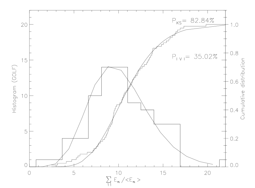
Figure 10: Histogram (15 bins) of $\Upsilon_{11,78}$ and cumulative distribution, compared to a $\Gamma_{11}$ distribution for GOLF (above) and IPHIR (below). In the IPHIR case, the dashed lines correpond to the theoretical distribution $\Gamma_{11}^{\lambda=.25}$.

The difference between the two series appears on the distribution $\Upsilon_{11,78}$ shown in Fig. 10, where both the variance and the KS tests indicate that the modes are likely to be less independent in IPHIR data than in GOLF data.
The tests applied to GOLF data are compatible with the null hypothesis ($P_{|V|}=35.0\%$, $P_{KS}=82.8\%$), which is consistent with the results of Sect. 3.
By contrast, the same tests applied to IPHIR data reject the null hypothesis with a $99.32\%$ confidence level with the variance test, and a $95.72\%$ confidence level for the KS test ($P_{|V|}=0.68\%$, $P_{KS}=4.28\%$).

4.3 Test of the “$\lambda$-hypothesis”

While the cumulative distribution $\Upsilon_{11,78}$ of GOLF does not show any systematical trend when compared to $\Gamma_{11}$, the cumulative distribution $\Upsilon_{11,78}$ of IPHIR shows a clear trend. This trend is successfully suppressed when compared to the distribution $\Gamma_{11}^{0.25}$ (Fig.  10). Fig. 11 shows that within our simple model, the signal of IPHIR would be absolutely normal as regards our tests ($P_{|V|}=85.0\%$, $P_{KS}=42.6\%$) if a fraction $\lambda=25\%$ of each mode energy were common to all the modes, correponding to a mean correlation ${\cal C}=6\%$.
Error bars are obtained by varying the parameter $\lambda$: the variance test leads to ${\cal C}=6.1\pm 3.3\%$, while the KS test obtains ${\cal C}=10.7\pm 5.9\%$.
Moreover, the correlation computed from Eq. (9) with the statistical error given by Eq. (30) is ${\cal C}=5.0\pm 3.6\%$. Although this analytical estimate is less reliable than the tests based on Montecarlo simulations (Eq. (30) neglects the error in estimating the mean energy of each mode), it is useful as a quick check of the results.
It is therefore comforting to notice, as can be seen in Fig. 11, that the range of correlations defined by these three methods overlap in the range $4.8\%<{\cal C}<8.6\%$, correponding to $21.9\%<\lambda<29.3\%$. Of course, this overlapping region cannot be directly interpreted in terms of a standard deviation. We shall adopt the conservative range obtained with the KS test, which takes the full distribution into account: ${\cal C}=10.7\pm 5.9\%$, corresponding to a fraction $\lambda=31.3\pm 9.4\%$.

Figure 11: Comparison of IPHIR data ($p=78$ points) with a theoretical distribution made of $k=11$ modes containing a fraction $\lambda={\cal C}^{1/2}$ of energy in common. The vertical dotted lines delimit the range of the correlation coefficient determined by Eq. (9). The KS test remain inside the upper $68.3\%$ region for ${\cal C}=10.7\pm 5.9\%$, corresponding to a fraction $\lambda=31.3\pm 9.4\%$.

4.4 Additionnal checks

In order to check the possibility that the correlation might come from a multiplicative noise (such as due to a pointing noise), we have computed the correlation between $11$ windows of noise centered $20\mu Hz$ (resp. $27\mu Hz$) to the right of each mode. This test indicates that the noise itself is not correlated, with $P_{|V|}=77.2\%$ and $P_{KS}=25.5\%$ (resp. $P_{|V|}=68.4\%$ and $P_{KS}=34.3\%$).
We have checked the effect of changing the size of the filtering window to 4 $\mu$Hz (no noise, but low statistics of 52 points) and 8 $\mu$Hz (good statistics of 106 points, but IPHIR is influenced by the noise). While a smaller filtering window still favours $\lambda\sim 25\%$, a larger window takes into account a significant fraction of uncorrelated noise, as expected, resulting in a slightly lower value of $\lambda$.
One might also suspect that the discrepency between the IPHIR distribution $\Upsilon_{11,78}$ and a $\Gamma_{11}$ distribution is due to the mode $l=1$, $n=22$ which is not well fitted by an exponential distribution (see Fig. 8). Nevertheless, performing the same analysis without this particular mode leads to the same conclusion: $P_{|V|}=0.28\%$ and $P_{KS}=6.9\%$ if $\lambda=0$, while $P_{|V|}=78.2\%$ and $P_{KS}=38.5\%$ if $\lambda=25\%$.

5 Conclusion

The exponential nature of the energy distribution of each mode has been used to compute their mean correlation coefficient with a consistent error bar.
Two tests based on Montecarlo simulations, and one analytical formulae, applied to 310 days of GOLF data, support the null hypothesis of no mean correlation among the modes $17\leq n\leq 25$, $l=0,1$, with an accuracy of ${\cal C}=0\pm 0.6\%$.
Our analysis of the modes correlation in IPHIR data, using these statistical tools, gives an accurate statistical support to the tentative conclusions of Baudin et al. (1996). The variance test rejects the null hypothesis with a $99.3\%$ confidence level.
The presence of a clear correlation among p-mode energies in IPHIR data strongly constrains the standard picture of stochastic excitation. If really of solar origin, it suggests the existence of an additional source of excitation, other than the granules. We have built a one parameter model of random excitations separated by a time comparable to the damping time of the modes, added to the usual granule excitations. IPHIR data are fully compatible with this “$\lambda$-hypothesis”, if a fraction $\lambda=31.3\pm 9.4\%$ of each mode energy is due to this additionnal source of excitation, resulting in a mean correlation ${\cal C}=10.7\pm 5.9\%$ among the modes.
On the other hand, the absence of correlation in GOLF data support the standard picture of stochastic excitation by the granules only.
This difference between IPHIR and GOLF data can be interpreted as a change from $\lambda=31.3\pm 9.4\%$ in IPHIR data to less than $8\%$ in GOLF data.
This evolution could be related to the change in magnetic activity, since the GOLF data correspond to a period close to the solar minimum while the IPHIR data correspond to a period closer to the solar maximum. If this is true, a confirmation will be obtained by performing this same analysis on GOLF data when we approach the solar maximum, in a couple of years. VIRGO data will also be useful in order to identify the possible role of the measurement techniques (velocity/intensity) in the determination of the correlation.
However, the mechanism by which the magnetic field influences the excitation of the modes, i.e. the nature of these hypothetical exciting events remains to be explored in more detail.

Appendix A Extraction of the time evolution of the energy

Let us consider the real displacement $y(t)$ filtered through a double window with a width $\Delta\omega$, centred on the frequencies $\pm\omega_{0}$:

$$y(t)\equiv\int_{\omega_{0}-{\Delta\omega\over 2}}^{\omega_{0}+{\Delta\omega\over 2}}{\hat{y}}(\omega){\rm e}^{i\omega t}{\rm d}\omega+\rm c.c.,$$ (14)

where $\rm c.c.$ is the complex conjugate of the first term. By analogy with an oscillator of eigenfrequency $\omega_{0}$, the energy is defined as the sum of a kinetic and a potential part:

$${E\over M}(t)\equiv{1\over 2}(v^{2}+\omega_{0}^{2}y^{2}).$$ (15)

From Eq. (1) and (14), the filtered displacement and velocity can be written as follows:

$$y(t) = {\cal R}{\rm eal}\left\{2\;{\rm e}^{i\omega_{0}t}f_{y}(t)\right\},$$ (16)

$$v(t) = {\cal R}{\rm eal}\left\{2\;{\rm e}^{i\omega_{0}t}f_{v}(t)\right\},$$ (17)

$${E\over M}(t) = |f_{v}|^{2}+\omega_{0}^{2}|f_{y}|^{2}$$ (18)

$$+{\cal R}{\rm eal}\left\{{\rm e}^{2i\omega_{0}t}(f_{v}^{2}(t)+\omega_{0}^{2}f_{y}^{2}(t))\right\}.$$

We first deduce from the relation $v\equiv{\rm d}y/{\rm d}t$ that $f_{v}$ and $f_{y}$ are related as follows:

$$f_{v}(t) = i\omega_{0}\int_{-{\Delta\omega\over 2}}^{+{\Delta\omega\over 2}}{\hat{y}}(\omega_{0}+\omega){\rm e}^{i\omega t}\left(1+{\omega\over\omega_{0}}\right){\rm d}\omega,$$ (19)

$$= i\omega_{0}f_{y}(t)\left\{1+{\cal O}\left({\Delta\omega\over\omega_{0}}\right)\right\}.$$ (20)

From Eq. (1), the non-zero Fourier components of $f_{y}$ (and $f_{v}$) correspond to frequencies between $-\Delta\omega/2$ and $+\Delta\omega/2$. If, as is usually the case, $\Delta\omega\ll\omega_{0}$, the high frequency oscillations of $\exp\pm 2i\omega_{0}t$ are well separated from the slower variations of $f_{y}(t)$ and $f_{v}(t)$, and Eq. (18) is approximated by Eq. (2).

Appendix B One parameter model of correlated modes

The amount of energy which is coherent among the modes can be estimated by constructing a simple one-parameter model as follows. Indexing the modes by $j\in\{1,k\}$, we assume that the velocity residual of each mode $V_{j}(t)=v_{j}(t)+\alpha_{j}v_{0}(t)$ is made of a superposition of two independent signals, where $v_{0}(t)$ is common to all the modes, and all the $v_{j}(t)$, $j\in\{0,k\}$, are independent.
Using the filtering method described in Section 1, we introduce the parameter $\theta_{j}$ as:

$$f_{V_{j}}(t) = f_{v_{j}}(t)+\alpha_{j}f_{v_{0}}(t)$$ (21)

$$\equiv {\sigma(f_{V_{j}})\over 2}\left(\cos\theta_{j}\left|\begin{array}[]{l}r_{j}\\ i_{j}\end{array}\right.+\sin\theta_{j}\left|\begin{array}[]{l}r_{0}\\ i_{0}\end{array}\right.\right),$$ (26)

where $(r_{j},i_{j})$, $j\in\{0,k\}$, are independent normalized normal distributions. The quantity $\lambda_{j}\equiv\sin^{2}\theta_{j}$ can be interpreted as the ratio of the energy in the common signal to the total energy of the mode. We denote by $e_{j}$ the energy of the signal filtered in the Fourier space, normalized to its mean value:

$$e_{j}\equiv{1\over 2}\left\{(r_{j}\cos\theta_{j}+r_{0}\sin\theta_{j})^{2}+(i_{j}\cos\theta_{j}+i_{0}\sin\theta_{j})^{2}\right\}.$$ (27)

The correlation between two modes ${\cal C}_{i,j}$ is then:

$${\cal C}_{i,j}=\lambda_{i}\lambda_{j}.$$ (28)

For the sake of simplicity, $\lambda_{j}\equiv\lambda$ is assumed to be independent of the mode $j$. This is equivalent to assuming that the correlation is uniform among the modes.
The sum $\Upsilon_{k}$ of the normalized energies is defined as:

$$\Upsilon_{k}\equiv\sum_{j=1}^{k}e_{j}.$$ (29)

The variance of the estimator of the variance depends on the fourth moment of the distribution, and is equal to:

$$\sigma_{\rm var}^{2}={2k(k+3)\over p}+$$

$${2k(k-1)\lambda^{2}\over p}[2(k+9)+12(k-2)\lambda+(4k^{2}-10k+9)\lambda^{2}].$$ (30)

Let us show that the higher order moments $\mu_{l}$ of the distribution $\Upsilon_{k}$ vary like $\lambda^{2}$, to first order.

$$\mu_{l}\equiv\left\langle(\Upsilon_{k}-k)^{l}\right\rangle,$$ (31)

where $\langle\;\rangle$ denotes the expectation value of the distribution. As the transformation $\theta\to-\theta$ does not change the distribution defined by Eq. (27), only the even powers of $\sin\theta$ can contribute to $\mu_{l}$. It can therefore be expanded into powers of $\lambda=\sin^{2}\theta$. Let us develop the product in Eq. (31) and prove that the term of order $\lambda$ is zero. We use below the special relation between the centred moments $\tilde{\mu}_{l},\tilde{\mu}_{l-1},\tilde{\mu}_{l-2}$ of a $\Gamma_{k}$-distribution of order $k$:

$$\mu_{l} = \tilde{\mu}_{l}+A\lambda+{\cal O}(\lambda^{2}),$$ (32)

$$A = \left\langle{l(l-1)\over 2^{l-1}}\left(\sum_{j=1}^{k}r_{0}r_{k}+i_{0}i_{k}\right)^{2}\left(\sum_{j=1}^{k}r_{k}^{2}+i_{k}^{2}-2\right)^{l-2}\right\rangle$$ (33)

$$-l\tilde{\mu}_{l}$$

$$= l(l-1)\left(\tilde{\mu}_{l-1}+k\tilde{\mu}_{l-2}\right)-l\tilde{\mu}_{l}$$ (34)

$$= 0.$$ (35)

Let us now show that the probability density $\Gamma_{k}^{\lambda}(x)$ of $\Upsilon_{k}$ also varies like $\lambda^{2}$, to first order.
Given the Eqs. (27)-(29) defining $\Upsilon_{k}$, we can expand $\Gamma_{k}^{\lambda}(x)$ in powers of $\lambda$.

$$\Gamma_{k}^{\lambda}(x)=\Gamma_{k}(x)+\lambda g(x)+{\cal O}_{x}(\lambda^{2}).$$ (36)

The moment of order $l$ is defined as:

$$\mu_{l} \equiv \int_{-\infty}^{+\infty}(x-k)^{l}\Gamma_{k}^{\lambda}(x){\rm d}x$$ (37)

$$= \tilde{\mu}_{l}+\lambda\int_{-\infty}^{+\infty}(x-k)^{l}g(x){\rm d}x+{\cal O}_{x}(\lambda^{2}).$$ (38)

The fact that every moment $\mu_{l}$ varies at least like $\lambda^{2}$ (Eq. 35) implies:

$$\int_{-\infty}^{+\infty}(x-k)^{l}g(x){\rm d}x=0.$$ (39)

The only function $g(x)$ satisfying Eq. (39) for any value of $l$ is $g\equiv 0$. Therefore both $\Gamma_{k}^{\lambda}(x)$ and its primitive (i.e. the cumulative distribution of $\Upsilon_{k}$ involved in the KS test) vary like $\lambda^{2}$ to first order.
We conclude that the sensitivity of the KS test is comparable to the sensitivity of the variance test.

References

- (1) Baudin F., Gabriel A., Gibert D., 1994, A&A 285, L29
- (2) Baudin F., Gabriel A., Gibert D., Pallé P.L., Regulo C., 1996, A&A 311, 1024
- (3) Baudin F., Gabriel A.H., Garcià R., Foglizzo T., Gavryusev V., Gavryuseva E., Gough D., Ulrich R.K. and the GOLF Team, 1997, Proceedings of the IAU Symposium 181, F-X Schmider & J. Provost Eds, Observatoire de Nice, France, in press
- (4) Chang H.-Y. 1996, PhD Thesis, University of Cambridge
- (5) Chang H.-Y., Gough D., 1995, in GONG’94: Helio- and Astero-seismology, ASP Conference Series, Ulrich R.K., Rhodes E.J. Jr. and Däppen W. Eds, Vol 76, p. 512
- (6) Chaplin W.J., Elsworth Y., Howe R., Isaak G.R., McLeod C.P., Miller B.A., 1995, proceedings of Fourth SOHO Workshop: Helioseismology, Pacific Grove, California, 2-6 April 1995 (ESA SP-376), p. 335
- (7) Gavryusev V.G., Gavryuseva E.A., 1997, Solar Physics, in press
- (8) Goldreich P., Keeley D.A., 1977, ApJ 211, 934
- (9) Kumar P., Franklin J., Goldreich P., 1988, ApJ 328, 879
- (10) Lazrek M., Baudin F., Bertello L., Boumier P., Charra J., Fierry-Fraillon D., Fossat E., Gabriel A.H., García R.A., Gelly B., Gouiffes C., Grec G., Pallé P.L., Pérez Hernandez F., Régulo C., Renaud C., Robillot J.-M., Roca Cortés T., Turck-Chièze S., Ulrich R.K. 1997, Sol. Phys. special SOHO issue, in press
- (11) Toutain T., Fröhlich C., 1992, A&A 257, 287
- (12) Woodard M., 1984, PhD Thesis, University of California, San Diego