The distribution of nearby stars in phase space mapped by Hipparcos

Abstract

Hipparcos data provide the first, volume limited and absolute magnitude limited homogeneous tracer of stellar density and velocity distributions in the solar neighbourhood. The density of A-type stars more luminous than $M_{v}=2.5$ can be accurately mapped within a sphere of 125 pc radius, while proper motions in galactic latitude provide the vertical velocity distribution near the galactic plane. The potential well across the galactic plane is traced practically hypothesis-free and model-free. The local dynamical density comes out as $\rho_{0}=0.076\pm 0.015~{}M_{\sun}~{}{\rm pc}^{-3}$ a value well below all previous determinations leaving no room for any disk shaped component of dark matter.

1 Introduction

All the data used here were collected by the Hipparcos satellite ([ESA, 1997]). Individual stellar distances within more than 125 pc were obtained with an accuracy better than 10$\%$ for almost all stars brighter than $m_{v}=8.$, together with accurate proper motions. Based on these data, a unique opportunity is offered to revisit stellar kinematics and dynamics; any subsample of sufficiently luminous stars is completely included within well defined distance and luminosity limits, providing a tracer of the local density-motion equilibrium in the galaxy potential: a snapshot of the phase space. We have selected a series of A-F dwarf samples ranging from $M_{v}=-1.0$ down to $M_{v}=4.5$. Completeness is fixed within 50 pc over the whole magnitude range and within 125 pc at the luminous end ($M_{v}\leq 2.5$). In this series of papers we shall investigate such samples in terms of density and velocity distribution small scale inhomogeneities addressing the problem of cluster melting and phase mixing.

The expected first order departure to homogeneity is the potential well across the galactic plane. This problem is well known in galactic dynamics; it is usually referred to as “the $K_{z}$ problem”, where $K_{z}$ means the force law perpendicular to the galactic plane. The $K_{z}$ determination and subsequent derivation of the local mass density $\rho_{0}$ has a long history, nearly comprehensive reviews can be found in [Kerr & Lynden-Bell (1986)] covering the subject before 1984 and in [Kuijken (1995)] since 1984. Early ideas were given by Kapteyn (1922), while Oort (1932) produced the first tentative determination.

The essence of this determination is quite simple: the kinetic energy of stellar motions in the z direction when stars cross the plane fixes their capability to escape away from the potential well. Given a stellar population at equilibrium in this well, its density law $\nu(z)$ and velocity distribution at plane crossing $f(w_{0})$ are tied to each other via the $K_{z}$ or the potential $\phi(z)$. Under quite general conditions the relation that connects both distributions is strictly expressed by Eq. (1).

$$\nu(\phi)=2\int_{\sqrt{2\phi}}^{\infty}{f(|w_{0}|)~{}w_{0}~{}{\rm d}w_{0}\over\sqrt{w_{0}^{2}-2\phi}}$$ (1)

This integral equation and its validity conditions are established and discussed in detail by [Fuchs & Wielen (1993)] and [Flynn & Fuchs (1994)]. There is no specification as to the form of distribution functions $f$ and $\phi$ except smoothness and separability of the z component.

Given $\nu(z)$ and $f(w_{0})$, $\phi(z)$ can be derived. Then according to Poisson equation, the local dynamical density comes out as

$$\rho_{0}={1\over 4\pi G}({\rm d}^{2}\phi/{\rm d}z^{2})$$ (2)

Early determinations of $\rho_{0}$ ([Oort, 1960]) were as high as $0.18\,M_{\sun}\,{\rm pc}^{-3}$ while the total mass density of stars and interstellar matter would not exceed $0.08\,M_{\sun}\,{\rm pc}^{-3}$. The discrepancy between these two figures latter re-emphasised by J. Bahcall and collaborators (1984ab, 1992), came into the picture of the dark matter controversy to make it even darker. While the local density of standard “dark halos” required to maintain flat rotation curves of galaxies away from their center would hardly exceed 0.01, such ten times larger densities could only be accounted for in rather flat components which composition and origin could not be the same. Following Bahcall’s claim, several attempts were made to reduce the intrinsic inaccuracy of the dynamical mass determinations in particular [Bienaymé et al (1987)], used a complete modelisation of the galaxy evolution to tie the $K_{z}$ determination to star counts, [Kuijken & Gilmore (1989)] used distant tracers of K type stars to determine not the local volume density but the integrated surface density below 1 kpc, [Flynn & Fuchs (1994)] pointed at difficulties in relation with the underlying dynamical approach. Most concluded that there was no conclusive evidence for a high dynamical density if all causes of errors were taken into account.

The local mass density of observable components (the observed mass) can hardly exceed $0.08M_{\sun}{\rm pc}^{-3}$ out of which a half stands for stars which local luminosity function is reasonably well known. The mass density of interstellar gas and dust is not so easily accessed since the bulk of it, molecular hydrogen, can only be traced via CO and the ratio CO/$\rm{H_{2}}$ is not so well established. Also interstellar components are basically clumpy and distances poorly known: it is not so easy to define a proper volume within which a density makes sense. A conservative range for the observed mass density should be $[0.06,0.10]$ including 0.04 for stars.

Nevertheless, so far the discrepancy used to be charged to the dynamical density since the determination of this quantity involved many difficulties, most poorly controlled :

• Tracer homogeneity: first of all, the determination require that a suitable tracer can be duly identified. A criterion independent of velocity and distance should allow to detect and select all stars matching the tracer definition. This was hardly achieved by spectral surveys which completeness and selectivity degrade as magnitude grows.

• Stationarity: in order for the tracer to make dynamical sense, it should be in equilibrium in the potential. Youngest stars which velocities reflect the kinematics of the gas at their birth time do not fulfill this requirement.

• Undersampling: one searches for the bending of density laws caused by gravitation along the z direction. This imposes not only that tracer densities can be determined, but also that they can be determined at scales well below the typical length of the bending. This means that the tracer should be dense enough in the region studied. Most determinations so far rely upon sample surveys in the galactic polar caps, resulting in “pencil beam” samples quite inappropriate to trace the density near the plane ([Crézé et al, 1989]). When the bending is traced at large distances from the plane as in [Kuijken & Gilmore (1989)], one gets information on the surface density below a certain height. A comparison of this surface density with the local volume density involves modeling hypotheses. Another associated effect can be generated by a clumpy distribution of the tracer even stationary if the tracer includes clusters or clumps the statistics of densities and velocities may be locally biased. Other problems arise from the velocity distribution sampling.

• Systematic errors: out of necessity before Hipparcos, all previous studies used photometric distances. Uncertainties in the calibration of absolute magnitudes resulted in systematic errors in density determinations. This is particularly true for red giants which are not at all a physically homogeneous family and show all but normal absolute magnitude distributions: it is striking that calibrations based on different samples provide discrepant calibrations outside the range permitted by formal errors. This produced both biased density distributions and uncontrolled effects in selecting volume limited samples.

• Random errors: distances and velocities were also affected by random measurement errors. Even perfectly calibrated, standard errors of photometric distances based on intermediate band photometry would hardly get below 20%.

Hipparcos data solve nearly all the problems quoted above: instead of “pencil beam” tracers at high galactic latitudes which distribution is only indirectly related to the local $K_{z}$, what we get here is a dense probe inside the potential well.

The samples were preselected within magnitude limits inside the completeness limit of the Hipparcos survey program ([Turon & Crifo, 1986]). It includes all stars brighter than $m_{v}$ = 8.0 (7.9 at low latitudes) with spectral types earlier than G0, stars with no or poorly defined spectral types were included provisionally.

Within this coarse preselection, sample stars were eventually selected on the basis of their Hipparcos derived distance, magnitude and colour. So the only physical criterion is absolute magnitude while the sample is distance limited on the basis of individual parallaxes. Within 125 parsecs, Hipparcos parallaxes provide individual distances with accuracies better than 10 percent for over ninety percent of the sample. Distances are individual and free from calibration errors. Samples are dense, typical inter-star distances are less than 10 pc. This is suitable to trace density variations which typical scales are of the order of hundred parsecs. Thanks to this high tracer density, difficulties related to clumpiness can be monitored through appropriate analysis of local density residuals. Stationarity considerations can also be monitored since W velocities are available for stars everywhere in the volume studied.

The main characteristics of the tracer samples are reviewed in section 2. In order to take full benefit of this new situation, an original method has been developed to analyze the densities. The statistical aspects of this method based on single star volumes (volume of the sphere extending to the nearest neighbour) are described in section 3 yielding a model free view of the potential well. Then an estimate of the local mass density of matter is produced (section 4). Consequences in terms of galactic structure and dark matter distribution are reviewed in conclusion (section 5).

2 The Hipparcos Sample

2.1 Sampling definition

The sample was pre-selected from the Hipparcos Input Catalogue ([ESA, 1992]), among the “Survey stars”. The Hipparcos Survey delimitation is described in full detail in Turon & Crifo (1986). For spectral types earlier than G5 the limiting magnitude is $m_{v}\leq~{}7.9+1.1sin|b|$. It is complete within those limits so far as the apparent magnitudes were known. Inside the Hipparcos Survey, the phase space tracer sample has been first given a coarse limitation: spectral types later than A0 and earlier than G0, luminosity class V through IV. Stars with uncertain or undefined luminosity classes were kept in the sample at this stage. Within this pre-selection, the final choice was based on Hipparcos magnitudes ($m_{v}<8.0$), colours ($-0.1~{}\leq~{}B-V~{}\leq~{}0.6$) and parallaxes ($\pi~{}\leq~{}8~{}{\rm mas}$). Then a series of subsamples were cut in absolute magnitude and distance in such a way that each subsample is complete for the adopted colour range within a well defined sphere. The resulting sample characteristics are summarized in Tab.(1). The sample designation system is straightforward: h125 means stars within 125 pc, under the apparent magnitude condition $m_{v}<8.0$, imposes not to consider stars less luminous than $M_{v}\leq 2.5$. All stars of sample h125 closer than 100 pc are included in sample H100 and so on. Samples named k… come from the corresponding h… samples but the identified cluster stars have been removed. The typical density of each sample estimated as the inverse of the average single star volume is given in the last column of Table 1. The corresponding typical interstar distance of e.g. tracer h125 is 8.8 pc.

Table 1: Main sample characteristics. M${}_{v\ lim}$ the limiting absolute magnitude, d_lim the limiting distance, N the number of stars, $<\nu>$ the mean number density.

Sample	M${}_{v\ lim}$	dlim	N	$<\nu>$
		(pc)		(10${}^{-5}\cdot$pc-3)
h125	$\leq$ 2.5	125.9	2977	48
k125	$\leq$ 2.5	125.9	2643	42
H100	$\leq$ 3.0	100.0	2677	88
K100	$\leq$ 3.0	100.0	2385	77
H80	$\leq$ 3.5	79.4	2336	152

2.2 Completeness

With this method, the sample limits do not rely upon pre-Hipparcos data except for the faintest stars next to the edge of each sphere, some of those might have been missed due to the limited accuracy of pre-Hipparcos magnitudes. The method may look a naive one since there are now sophisticated algorithms to correct estimations for censored data, (see for instance [Ratnatunga & Casertano, 1991]) but it is the only one that does not make assumptions as to the absolute magnitude distribution of the stars. All previous investigations did assume that the absolute magnitudes of stars sharing a certain spectral or photometric characteristic are normally distributed around a common mean value.

Figure 1: $M_{v}/V-I$ diagram for the global tracer sample (see section 2.1).

Figure 2: Absolute magnitude distribution of tracer stars in a series of colour range.

Figures 1 and 2 give a quantitative illustration of the risks involved: the absolute magnitude distributions of dwarfs within four V-I ranges show an obvious asymmetry while in the reddest part, the luminosity distribution spans over more than two magnitudes. This means that however accurately the apparent magnitude can be measured, the uncensoring correction would be much more uncertain than other error factors.

With the approach adopted here, Fig. 3 shows the $M_{v}$/distance distribution of the global sample, the neat border follows simply the line $m_{v}=8$; the censoring effects are maximum along this line. Our subsamples are cut along lines parallel to the axes of this plot, so they reach the censoring line only at the bottom right corner of each zone.

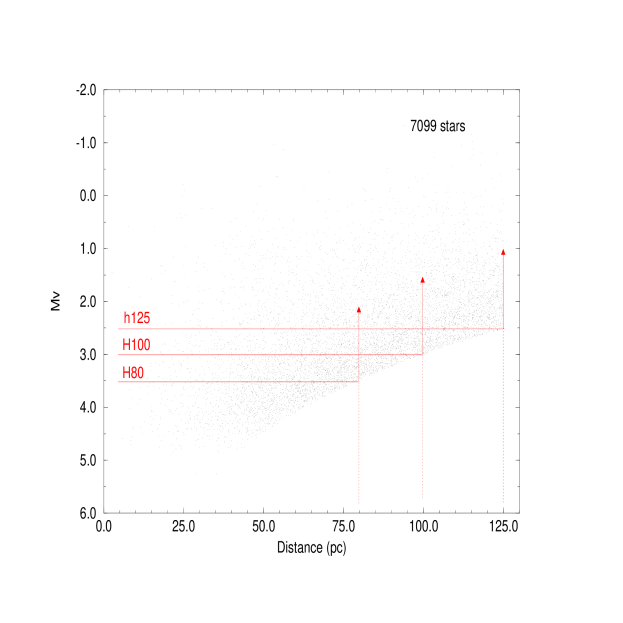
Figure 3: $M_{v}$/distance diagram for the global sample. See Table 1 for sample definitions.

Since the accuracy of Hipparcos magnitudes is far beyond the necessities of this study, the sampling biases can only result from two effects: the parallax errors which, however unprecedently small are still of the order of $10\%$ beyond 100 pc, and the stars lost at the time of the early selection due to the inaccuracy of apparent magnitudes available then. Concerning the second effect, it can only result in stars being omitted near the edge of the sample. The residual effect of apparent magnitude incompleteness can only affect the faintest magnitudes at the edge of each sample sphere, since the single star volume used in sections 3 and 4 as statistics for the density estimation are local statistics, it is easy to keep such effect under control in the study of residual, furthermore this kind of incompleteness if important would bias the estimation towards making the potential well even shallower than observed.

2.3 Distance errors

The other possible source of bias left is generated by distance errors. Figure 4 shows the distribution of parallax errors versus distance for sample h125 which, extending to 125 pc is the most severely affected by distance errors. This is still a moderate effect: one can see on the figure that only a handful of parallax errors exceed 15$\%$. Parallaxe errors are Hipparcos formal errors. All feasible external tests able to check the actual accuracy show that these formal errors are if something a little pessimistic ([Arenou et al, 1995]) with respect to previous studies of the density trends.

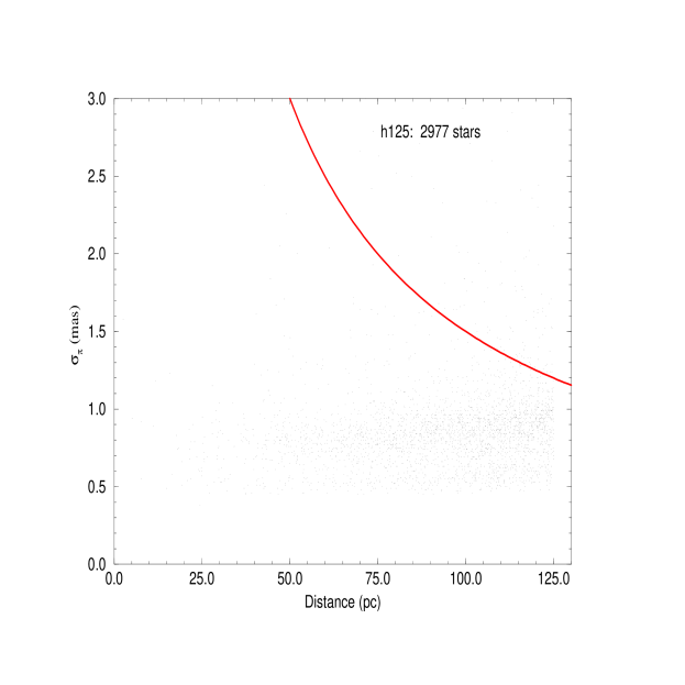
Figure 4: Formal parallax standard errors versus distance. Distance errors are larger than 15$\%$ for stars above the line.

3 Mapping the tracer density and the potential well

The essential choice of this investigation is to stick as closely as possible to observations. Whatever the velocity distribution $f(w_{0})$, once an homogeneous tracer has been defined, that is once a selection criterion has been defined uncensored with respect to velocities and positions, Eq. (1) expresses the correspondence between the tracer density law and the potential as a plain change of variables. So if there is a potential well to be found in the data, it must appear as a density peak. If we can map the density trend model free, we’ll get a picture of the potential well.

3.1 Single star volume statistics

The tracer should be dense enough for the typical distances between tracer stars to be small with respect to the typical scale of density variations. Under this assumption, at a place were the tracer density is $\nu$, the observed number of stars counted in any probe volume $V$ is a Poisson variate with expectation $V\cdot\nu$. Defining $v$ as the single star volume around one specific star (that is the sphere extending to the nearest neighbour), and introducing the quantity $x=v\cdot\nu$ we get a new variate which expectation is 1 and which probability distribution is exponential (Eq. (3)). It is the probability distribution of the distance between two events in a Poisson process under unit density.

$${\rm d}P(x)=\exp(-x)~{}{\rm d}x$$ (3)

and the probability distribution of the single star volume $v$ is

$${\rm d}P(v)=\nu\cdot\exp(-\nu\cdot v)~{}{\rm d}v$$ (4)

so the expectation of the single star volume is $1/\nu$, which makes it a suitable local statistics for the density. It is not a novel approach to use statistics based on nearest neighbour distances to investigate densities, but it is quite appropriate here since it turns out to provide a parameter free Maximum Likelihood estimator for the density by plain moving average of single star volumes. Also, single star volumes being a local measure of the inverse density at the position of each star, they offer the possibility to calculate individual density residuals. Checks can be made that deviations from average or model predicted values are randomly distributed and do not show unmodeled systematic trends.

3.2 Maximum Likelihood estimator

In a constant density sample, the plain average of single star volumes is a maximum likelihood statistics for the density: let $v_{i}$ be the single star volume around star i, according to Eq. (4) the log-likelihood of a sample of n stars $(i=1,n)$ under constant density $\nu$ is simply given by

$$\log L=\sum_{i=1,n}(\log(\nu)-\nu\cdot v_{i})$$ (5)

and the Maximum Likelihood is reached for

$${\rm d}\log L/{\rm d}\,\nu=0\\$$ (6)

which obvious solution is:

$$n/\nu=\sum_{i=1,n}v_{i}\\$$ (7)

$$\nu=1/<v_{i}>$$ (8)

this makes the moving average of $v_{i}$ along a parameter a maximum likelihood mapping of the density variations along this parameter, provided only that variations along other parameters are negligible.

3.3 Residual statistics

Furthermore, given a model or an estimate of $\nu$ near star i the quantities $x_{i}=\nu\cdot v_{i}$ are local “residuals” of the fit and their distribution under the assumed model should be exactly given, parameter-free, by Eq. (3). So the distribution of residuals provides an immediate test of the validity of the model including the fact that the density is smooth and do not include too many clusters or voids. This distribution can be tested over the whole sample or over any subset chosen to explore neglected parameters (e.g. the completeness near the edge of the sampling volume, completeness in apparent magnitude). In order to visualize the agreement (or disagreement) of the observed distributions we have used two representations: the histogram of the log residuals $y=log(x)$ which distribution according to Eq. (3) must be given by

$${\rm d}P(y)=\exp[y-\exp(y)]{\rm d}y\\$$ (9)

and the cumulative distribution of x:

$$H(X)=\int_{0}^{X}\exp(-x)\,{\rm d}x=1-\exp(-X)\\$$ (10)

Let $n_{i}$ be the rank of residual $x_{i}$ in a sample of N values, then according to Eq. (10),

$$n_{i}/N=1-\exp(-x_{i})\\$$ (11)

$$-\log(1-n_{i}/N)=x_{i}\\$$ (12)

In the following the residuals have been plotted as $-log(1-n_{i}/N)$ against $x_{i}$ producing what statisticians use to call exponential probability plots. On such plot, observed residual distributions that fail matching the expected exponential at any scale sign their existence by departures from the diagonal.

3.4 Edge effect

Around stars close to the edge of the completeness sphere, the single star volume is not anymore the full volume of the sphere to the nearest neighbour. The volume must be corrected for the part of the sphere outside the completeness volume (Fig. 5). Defining $d_{nn}$ the distance to the nearest neighbour, $d$ the Sun-star distance and $R$ the radius of the sample sphere, and defining the two spheres, one centered at sun position with radius $R$, the other at star position with radius $d_{nn}$, the corrected volume is calculated as $V_{cor}$ according to the following formulae. Angles $\theta_{1}$ and $\theta_{2}$ are the half apertures of the cones intercepting the intersection of the two spheres (summit at sun position for $\theta_{2}$, at star position for $\theta_{1}$).

$$\cos\theta_{2}=(d^{2}+R^{2}-d_{nn}^{2})/(2dR)$$ (13)

$$\sin\theta_{1}=(R/d_{nn})\sin\theta_{2}$$ (14)

$$V_{1}=(\pi/3)d_{nn}^{3}(2-3\cos\theta_{1}+\cos^{3}\theta_{1})$$ (15)

$$V_{2}=(\pi/3)R^{3}(2-3\cos\theta_{2}+\cos^{3}\theta_{2})$$ (16)

$$V_{cor}=(4/3)\pi d_{nn}^{3}-(V_{1}-V_{2})$$ (17)

Figure 5: Edge effect: geometry of the volume correction (shaded area) due to the part of the nearest neighbour volume outside the completeness volume.

3.5 Mapping the density

Single star volumes which are unbiased local estimates of the inverse tracer density have been computed for all the tracer samples described in Table 1. Defining x,y,z as a set of cartesian coordinates centered at the sun position, with z positive pointing towards $b=+90^{\circ}$, x positive towards the galactic center ($l=0^{\circ}$) and y towards $l=90^{\circ}$, each series of values was sorted along x, y and z successively and each resulting set smoothed by moving average along the sort parameter. Single star volumes are averaged over 101 neighbouring stars, producing parameter free maximum likelihood inverse density profiles. Figures 6 through 8 show the resulting profiles along x, y and z for our three most accurate and extended samples (namely samples h125, H100 and H80, according to definitions of section 2.1). In these figures the x and y plots are given only as references: since the sampling definition has spherical symmetry, any systematic effect along the z axis which would trace a sampling artifact rather than a real trend of the density would appear as well along the x and y axis.

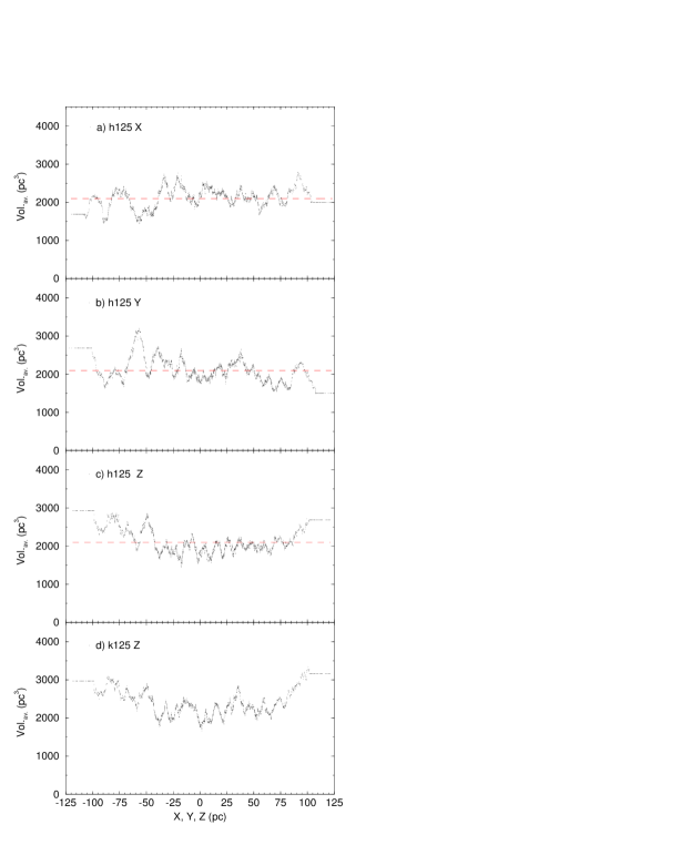
Figure 6: Single star volumes for A stars with $Mv\leq 2.5$ within 125 pc (sample h125) volumes in cubic parsecs are moving averaged along a) the x ( l = 0, b = 0), b) y (l = 90 , b = 0) and c) z (b = 90 ) directions. Moving averages are performed over 101 stars, so that random fluctuations are roughly one order of magnitude below that of raw data. d) shows in comparison the same kind of plot for sample k125 axis z, where cluster stars have been removed from sample h125. The bending due to the potential well in the galactic plane is clearly visible on plots c and d.

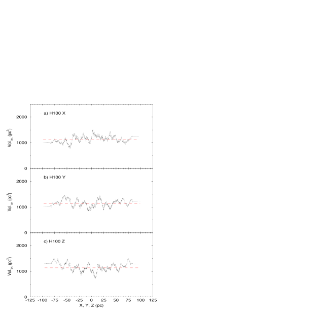
Figure 7: same as Fig. 6 sample H100.

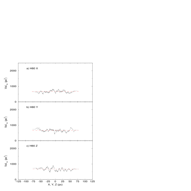
Figure 8: same as Fig. 6 sample H80.

At first glance only do the h125 and H100 profiles along the z axis show significant bending. Expectedly the youngest subsamples with the smallest velocity dispersions are also the most sensitive tracers. This is a direct mapping of the potential well. The next section will be dedicated to deriving quantitative consequences of this observation. Beforehand the result should be scrutinized in the light of two possible criticisms: biases in the inverse volume estimates at the edges of the sample and clumpiness effects among poorly mixed A stars.

Edge effects potentially related to completeness and/or to distance errors can be easily controlled: would they be responsible for the main part of the observed bending they would appear as well on the x and y plots. There is no such thing visible even at marginal level. In addition, any significant incompleteness at the edges would result in a density decrease driving the single star volume statistics up at the edges. As a result, the dynamical density derived below, once corrected for this effect, would be even smaller.

A more serious problem comes from the clumpiness of the distribution: young stars that dominate the most luminous samples are likely to be partly concentrated in clusters or clumps on scales of a few parsecs to a few ten parsecs. Such clumps must be suspected to distort the density profile. The fluctuations observed at small scales on figure 6 through 8 are not significant in this respect, they are the result of random fluctuations of single star volumes smoothed by the moving average process. The moving average introduces a strong self correlation in the series. As a result random fluctuations fake systematic ones on scales which are connected with the z ranges spanned by 101 neighbouring stars, but do not reflect these ranges in any simple way (it has something to do with the probability of getting one, two, three … extreme peaks within adjacent strips). Similar pictures are obtained on strictly uniform random simulations.

The only place where to check this effect is the statistics of residuals. Real clumps which are not plain random fluctuations in a uniform density are expected to sign their presence not by their local density which may not be very high locally on the average, but by the frequency of corresponding single star volume residuals (see section 3.3 for the definition of these residuals. Such an overfrequency is clearly visible on the bottom left wing of the histogram on figure 9a. In terms of cumulative distribution it is even more clear on figure 9b. A separate analysis of clustering has been performed by means of wavelet analysis (Chereul et al. to appear as paper II of this series) showing that no more than 8$\%$ out of stars in the h125 sample are involved in clumps. Removing only cluster members identified through proper motions we get sample k125. The z inverse density profile of this new sample is plotted on figure 6d, the profile is not strongly modified by removing cluster stars. On the residual plot (figure 9c) the residual anomaly at small scales vanishes definitely. So the inverse density profiles turn out quite robust to clumpiness effects. Furthermore we shall see in the following (section 4.2 and figure 13) that local mass density estimates based on the two samples (with or without cluster stars) are fully compatible. Also, once a suitable density model is found, the residual statistics of sample k125 (Figure 13b) do not show any significant feature that might signal undetected clumpiness left.

Figure 9: Inverse density residual distribution for the sample h125. Residuals are defined as y = ((single star volume) / average (101 stars)) a) histogram of $log~{}y$. The smooth line is the theoretical distribution. b) cumulative distribution of residuals (relative rank / expected rank of observed value). Departures from being parallel to the diagonal would sign under or over frequency of residuals at relevant scales. The presence of star clusters is visible at bottom left. c) same as b), cluster stars were excluded from the analysis (sample k125).

This gives confidence that the bending is real and that figures 6cd, 7c are the first ”image” of the galactic potential well. The remarkable feature here is that this well is extremely shallow. We shall see in the following that any substantial layer of dark matter contributing significantly in the local mass density would unmistakably sign its presence by deepening this well far beyond observed shapes. This is true also for samples H80 and H100 which, being dominated by elder stars are less affected by the clumpiness effect.

4 Estimating $\rho_{0}$

Solving Eqs. (1) and (2) for $\phi(z)$ can follow two different ways: a parametric approach and a non parametric one. Either were used on the above defined samples producing quite similar results.

• In the parametric approach, realistic mathematical forms are adopted for both $\phi(z)$ and $f(w_{0})$. Free parameters for $f(w_{0})$ can be determined by fitting the observed vertical velocity distribution then adopting $f(w_{0})$ free parameters for the potential, $\phi(z)$ can be derived from the observed density. The advantage of this approach is simplicity in so far as manageable formulae can be found to represent $f(w_{0})$. The cost is that results may be biased by the choice of the model. An advantage may be that systematic effects can be traced and individual residuals can be computed at the position and velocity of each star. This approach is developed in section 4.1.

• At the other end one can try to produce a purely numerical fit. Since this kind of fit is unstable to noise in the data, some regularization should be applied. This non parametric approach is developed in section 4.3.

4.1 Parametric approach: velocity analysis

The observed W vertical velocity distributions in the galactic plane were derived from Hipparcos proper motions in galactic latitude and parallaxes. For this analysis, samples were restricted to stars below $b=\pm 10\degr$ so that $\mu_{b}/\pi$ simply reflects the W tangential velocity.

W histograms of the four samples under consideration are shown on Fig. 10.

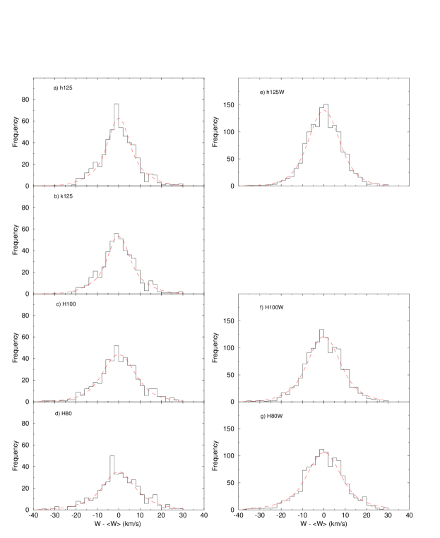
Figure 10: W velocity histograms from $\mu_{b}$ of low latitude stars (left hand column) and from space velocities of all stars with known radial velocities (right hand column); samples : h125 a),e) ; k125 b) ; H100 c), f) ; H80 d),g).

All four distributions show reasonable symmetry and smoothness with the following exceptions: h125 (Fig. 10a) shows pronounced spikes corresponding to clusters (spikes vanish in the histogram of k125) and a dissymmetry of large velocities (involving only 5 stars out of 456). The plain average $W_{0}$ has been estimated for all samples and appears quite stable suggesting that unsteady streaming motions characteristics of very young stars do not dominate. Under such conditions, the capability of the subsample of 536 low latitude stars to be representative of the whole population within 125 pc is questionable. Radial velocities have been compiled from the SIMBAD database in order to calculate space velocities for as many stars as possible. This resulted in a new velocity sample named h125W including 1366 stars spread in the whole sphere. The distribution of W velocity components has been studied in the following along the same lines as the other velocity sample.

A double gaussian centered model was fitted to each centered histogram using a simple maximum likelihood scheme:

the model fitted is

$${\rm d}P(w)=\{{\beta\over\sqrt{2\pi}~{}\sigma_{w1}}\exp[-{1\over 2}(w-<w>)^{2}/\sigma_{w1}^{2}]$$

$$+{1-\beta\over\sqrt{2\pi}~{}\sigma_{w2}}\exp[-{1\over 2}(w-<w>)^{2}/\sigma_{w2}^{2}]~{}\}~{}~{}{\rm d}w$$ (18)

and the maximum likelihood is searched for on $\beta$, $\sigma_{w1}$ and $\sigma_{w2}$.

There is no claim here that the kinematical mixture is isothermal. The idea is simply that, if this mixture can be accurately represented by a sum of gaussians, then there is a simple solution to the self consistent dynamical equilibrium, the force law and the local volume density can be solved for explicitly. The justification lays in the quality of the representation. This is also justified a posteriori by the fact that non parametric solutions do provide the same results.

Table 2 gives the maximum likelihood solutions for the four main samples investigated here. Two tests of the quality of the fit are given, one is the Kolmogorov-Smirnoff test: Pk is the observed Kolmogorov maximum distance, Pk(0.8) and Pk(0.95) are the 20$\%$ and 5 $\%$ rejection thresholds for this parameter. Obviously no rejection of the double gaussian representation can be supported at any meaningful level.

Table 2: Maximum Likelihood solutions for 2-gaussian fit of W velocity distribution.

Sample	N	W0	$\beta$	$\sigma_{w1}$	$\sigma_{w2}$	Pk	Pk(0.8)	Pk(0.95)
		km$\cdot s^{-1}$		km$\cdot s^{-1}$	km$\cdot s^{-1}$
h125	536	-6.53	0.60	10.40	4.46	.037	.046	.059
		(0.37)	(0.12)	(0.43)	(0.48)
h125W	1366	-6.94	0.50	10.67	6.08	.015	.029	.037
		(0.23)	(0.06)	(0.31)	(0.27)
k125	462	-6.83	0.60	10.4	4.20	.019	.050	.063
		(0.36)	(0.12)	(1.2)	(1.5)
H100	469	-6.39	0.70	11.46	4.79	.016	.049	.062
		(0.46)	(0.15)	(0.46)	(0.63)
H100W	1293	-6.93	0.50	12.49	6.39	.018	.029	.038
		(0.27)	(0.05)	(0.38)	(0.28)
H80	407	-5.84	0.60	13.17	5.81	.023	.053	.067
		(0.49)	(0.15)	(0.63)	(0.68)
H80W	1214	-6.88	0.50	14.46	6.60	.024	.031	.039
		(0.32)	(0.05)	(0.45)	(0.31)

The second test is given by probability plots (Fig. 11), velocity ranks in each sample are plotted against the theoretical cumulative probabilities of associated velocities: velocities distributed according to the estimated distributions would produce a strictly linear plot. So any deviation from linearity signs a failure of the double gaussian to represent observations.

Figure 11: W velocity probability plots (rank versus estimated cumulative probability) for samples of figure 10. Samples displaid just as on figure 10.

The likelihood surface is regular around each maximum, the dependence in $\sigma_{w1}$ and $\sigma_{w2}$ follows a nice parabola in log-likelihood indicating that the estimator behaves quite alike a gaussian variate in this region. Standard errors follow. The proportion $\beta$ is poorly determined although different values of $\beta$ may produce quite different M.L. estimates for $\sigma_{w1}$ and $\sigma_{w2}$. But the Likelihood levels reached do not deviate significantly from oneanother. A series of tests, not reported here, show that adopting any of those solutions, nearly equivalent in likelihood, do produce extremely close estimations of the dynamical density. Expectedly, what matters here, is the quality of the distribution representation, not the choice of specific functions. Eventually this conclusion is comforted by the excellent agreement between the results of the parametric and non parametric approach.

4.2 Parametric approach: density and potential analysis

Once we get models fitting W velocity distributions, which can be represented by double gaussians, the self consistent solution of Eqs. (1) and (2) can be expressed explicitly as

$$\ \nu(z)=\nu_{0}~{}[\,\beta~{}e^{-\phi(z)/\sigma_{w1}^{2}}+(1-\beta)~{}e^{-\phi(z)/\sigma_{w2}^{2}}\,]$$ (19)

Over the very small z range spanned by our 125 pc sphere, the potential well can be approximated at any required accuracy by a plain quadratic form

$$\phi(z)=\alpha\cdot(z-z_{0})^{2}$$ (20)

So, the density trend of a tracer $\nu(z)$ can be used to estimate $\alpha$, $\nu_{0}$ and $z_{0}$, once $\beta$, $\sigma_{w1}$ and $\sigma_{w2}$ have been derived from the velocities. The likelihood of a set of single star volumes under the assumption that the density trend is represented by Eqs. (19), (20), can be expressed by Eq. (21) similar to Eq. (5).

$$\log L=\sum_{i=1,n}~{}(~{}\log\nu(z_{i})-\nu(z_{i})\cdot v_{i}~{})$$ (21)

A maximum likelihood can be searched for $\alpha$, $\nu_{0}$ and $z_{0}$. According to the Poisson equation, the local dynamical density follows from $\alpha$ as:

$$\rho_{0}={1\over 2\pi G}~{}~{}~{}\alpha$$ (22)

Where $1\,/(2\pi G)=37.004$ if $\alpha$ is in $({\rm km\,s}^{-1}\,{\rm pc}^{-1})^{2}$ and $\rho_{0}$ in $M_{\sun}\,{\rm pc}^{-3}$.

Table 3 summarizes the results of solutions based on the three main samples (the separate solutions derived from samples without identified cluster stars do not produce different results). Three solutions are given for each sample: one is the 3-parameter M.L. solution, the other two are M.L. solutions for $\alpha$, $\nu_{0}$, while specific values have been forced for $z_{0}$.

Table 3: Maximum likelihood solutions for the local dynamical density from the three Hipparcos samples.

Sample	N	z0	$\beta$	$\sigma_{w1}$	$\sigma_{w2}$	1/$\nu_{0}$	$\rho_{0}$	Likelihood
		pc		km$\cdot s^{-1}$	km$\cdot s^{-1}$	($\star$/pc${}^{3})^{-1}$	M⊙/pc3
h125	2977	12.0	0.50	10.67	6.08	1887.67	0.075	-25666.64
		(6.0)				(35.63)	(0.009)
		0.0	0.50	10.67	6.08	1894.20	0.075	-25670.00
		(forced)				(35.70)	(0.010)
		-11.0	0.50	10.67	6.08	1926.14	0.059	-25676.31
		(forced)				(35.65)	(0.009)
H100	2677	4.0	0.50	12.49	6.39	1061.13	0.089	-21511.41
		(9.0)				(20.65)	(0.017)
		0.0	0.50	12.49	6.39	1061.52	0.089	-21511.71
		(forced)				(20.65)	(0.017)
		-10.0	0.50	12.49	6.39	1079.97	0.064	-21513.69
		(forced)				(20.87)	(0.016)
H80	2336	13.0	0.50	14.46	6.60	631.57	0.076	-17485.54
						(13.20)	(0.028)
		0.0	0.50	14.46	6.60	642.95	0.046	-17487.20
		(forced)				(13.38)	(0.031)
		-10.0	0.50	14.46	6.60	654.98	0.040	-17487.65
		(forced)				(13.55)	(0.028)

All three parameter solutions produce unexpected positive values for the z coordinate of the galactic plane. That is, the Sun would be very slightly south of the plane, in contradiction with most accepted values. We do not consider this result worth much consideration: for one thing the estimated local density does not change appreciably if $z_{0}$ is forced to 0 and even if it is pushed to a more classical $z_{0}=-10$, the estimated density decreases. For the other thing, there is certainly some clumpiness among the youngest stars in this sample which may blur the shape of the potential well the more so as this well turns out shallower than expected. Since it is not possible to evaluate accurately this effect we shall consider it as an intrinsic limitation of this determination. Accordingly the adopted solution is the weighted mean of M.L. solutions (weights proportional to inverse square standard errors), but error bars are extended in order to include all main solutions of Table 3.

$$\rho_{0}~{}=~{}0.076~{}\pm~{}0.015~{}M_{\sun}~{}{\rm pc}^{-3}$$ (23)

Based on this value and on the velocity distributions obtained in section 4.1, predicted density models defined by Eq. (19) have been overplotted on the z moving average profiles of all three tracer samples (Fig. 12 a,b,c). For comparison, profiles corresponding to arbitrary densities $\rho_{0}~{}=~{}0.10~{}M_{\sun}~{}{\rm pc}^{-3}$ and $\rho_{0}~{}=~{}0.15~{}M_{\sun}~{}{\rm pc}^{-3}$ are added. Obviously, even under quite conservative hypotheses, none of the samples can be reconciled with such local densities. The existence of any substantial disk shaped dark matter would definitely push all three curves outside the acceptable range.

Figure 12: Calculated inverse density profiles under three different assumed values of the local mass density $0.076~{}M_{\sun}~{}{\rm pc}^{-3}$ (best estimate), $0.10~{}M_{\sun}~{}{\rm pc}^{-3}$ and $0.15~{}M_{\sun}~{}{\rm pc}^{-3}$ (from bottom to top on each plot). Based on Eq. (20) and the velocity distributions of sample h125 a), H100 b) and H80 c). For comparison, the corresponding moving average profiles are repeated from figures 6c, 7c, 8c.

The distributions of single star volume residuals under the three density models have been scrutinized against possible unmodeled systematic effects. Probability plots as defined in section 3.3 (Eq. (11)) are given in Fig. 13.

The first two plots on top show the probability plot of residuals for samples h125 and k125 . Clearly enough models based on local mass densities higher than 0.08 generate a systematic distortion of the cumulative distribution of residuals with respect to the expected one. There is a small excess of low residuals even with our best fit model, but this effect vanishes when cluster stars are removed (sample k125) This correction does not change the conclusions on the local mass.

At this stage , the validity of the simplified assumption made on the potential can also be tested. A square function in z has been adopted for the potential, meaning a linear $K_{z}$. This means some homogeneity of the mass distribution over a 100 parsecs scale. If a substantial fraction of the mass happened to be concentrated in a very thin layer, this approximation would not hold. The Hipparcos samples are the first able to test this hypothesis over such small scales. The test is provided by the statistics of single star residuals. Would the $K_{z}$ slope change significantly within the limits of the sample, then this statistics of subsamples at low z would not match the expectation for the same assumed $\rho_{0}$. This test is presented in the bottom parts of Fig. 13. Samples h125 and H100 were split in different subsamples selected by $z$ after restriction to a cylinder of radius $r$. Expectedly, the failure of models based on $\rho_{0}=0.10$ and beyond is enhanced at high z ($|z|>69~{}{\rm pc}$). But, even over the restricted range $|z|<69~{}{\rm pc}$ there is signal left in the residuals to reject high density solutions. The low z part of sample H100 ($|z|<55~{}{\rm pc}$) is unable to produce any discriminant signal.

These residual plots fully confirm the result that local total volume densities beyond $0.10~{}M_{\sun}~{}{\rm pc}^{-3}$ cannot be reconciled with the observed velocity-density distributions. Similar plots restricted to subsamples selected by distance or magnitude or colour do not show significant deviations that might sign the presence of major selection effects in the sampling.

In terms of mass model the assumed linear $K_{z}$ implies that the total mass density is constant close to the plane. Assuming that it is true only for half of the mass, for instance the stellar distribution and that the gas distribution follows a sharper gaussian distribution with a scale height of 75 pc we may determine the extra forth order term in the potential. Determining the amplitude of the potential on counts at 75 pc leads to a very small difference of 1/24 between the two models. The resulting error on the derived $\rho_{0}$ is negligible with respect to other uncertainties.

Figure 13: Cumulative distribution of residuals (relative rank versus expected relative rank at residual) for $\rho_{0}=0.076$, $\rho_{0}=0.10$ and $\rho_{0}=0.15$. Departures to the diagonal sign anomalies in residual frequency. Full samples h125 a) and k125 b). Sub-samples h125 c) $|z|\leq 69~{}{\rm pc}$ and $r<104~{}{\rm pc}$ ; d) $|z|>69~{}{\rm pc}$. Sub-samples H100 e) $|z|\leq 55~{}{\rm pc}$ and $r<83.5~{}{\rm pc}$; f) $|z|>55~{}{\rm pc}$.

4.3 Non parametric approach

The non parametric approach does not rely upon any particular mathematical model for the velocity distribution function nor the height density profile ([Pichon & Thiébaut, 1997]). That is: ideally we should try and solve self consistently Eqs. (1) and (2) for $\rho_{0}$, with functions $f(|w_{0}|)$ and $\nu(\phi)$ defined on a purely numerical basis (in the range investigated here, approximating $\phi(z)$ by a simple square function is well justified). However a pure numerical solution is unstable: a small departure in the measured data (e.g. due to noise) may produce drastically different solutions since these solutions are dominated by artifacts due to the amplification of noise. Some kind of trade off must therefore be found between the level of smoothness imposed on the solution in order to deal with these artifacts on the one hand, and the level of fluctuations consistent with the amount of information in the signal on the other hand. Finding such a balance is called the “regularization” ([Wahba & Wendelberger, 1979]) of the self consistency problem. Regularization allows to avoid over-interpretation of the data. Here we chose to regularize the non-parametric self consistency problem by requiring a smooth solution. This criterion is tunable so that its importance may be adjusted according to the noise level (i.e.  the worse the data quality is, or the sparser the sample is, the lower the informative contents of the solution will be and the smoother the restored distribution will be).

Under the assumption that the potential is separable, the proposed method yields a unique mean density compatible with the measurement of the velocity distribution perpendicular to the Galactic plane and the corresponding measured density profile.

The discretized integral equation

From the knowledge of the level of errors in the measurements and given the finite number of data points, it is possible to obtain $f(w)$ by fitting the data with some model. A general approach assumes that the solution can be described by its projection onto a complete basis of functions with finite support (here cubic splines) $\{e_{k}(w);k=1,\ldots,N\}$:

$$f(w)=\sum_{k=1}^{N}f_{k}\;e_{k}(w)\equiv{\mathbf{f}}\cdot{\mathbf{e}}\;.$$ (24)

where the $N$ parameters to fit are the weights $f_{k}$. Real data correspond to discrete measurements $z_{i}$ and ${w}_{j}$ of $z$ and $w$ respectively. Following the non-parametric expansion in Eq. (24), Eq. (1) becomes:

$$\rho_{i}\equiv\rho(z_{i})=\sum_{k=1}^{N}A_{i,k}(\alpha,z_{0})\;f_{k}\,,$$ (25)

with

$$A_{i,k}(\alpha,z_{0})=\int_{\sqrt{2\alpha z^{2}_{i}}}^{\infty}\frac{e_{k}(w)w}{\sqrt{w^{2}-2\alpha z^{2}_{i}}}\,{{\mathrm{d}}{w}}\,.$$ (26)

Since the relation between ${\mathbf{\tilde{\rho}}}\equiv\{\rho_{i}\}$ and ${\mathbf{f}}\equiv\{f_{k}\}$ is linear, Eq. (25) — the discretized form of the integral equation (1) — can be written in a matrix form:

$${\mathbf{\tilde{\rho}}}={\mathbf{A}}(\alpha,z_{0})\!\cdot\!{\mathbf{f}}$$ (27)

Here $z_{0}$ accounts for the relative offset in the position of the sun with respect to the galactic plane as defined by the Hipparcos sample to the measured density.

The Hipparcos sample gives access within a given sphere to a number of stars for which the velocity, $w$, and/or the altitude, $z$, is known. In other words the measurement yields a realization of the cumulative height density distribution and the cumulative velocity distribution. Indeed for each star at height $z$, within ${{\mathrm{d}}{z}}$ of the next star (once they have been sorted in height), we can associate a volume given by

$$\pi\,{{\mathrm{d}}{z}}\,R^{2}(1-z^{2}/R^{2})$$ (28)

where $R$ is the radius of the Hipparcos sphere; an alternative estimated local density for this star is given by the inverse of this volume. This density estimator yields a local density consistent with that derived in section 3. An estimate of its cumulative distribution is directly available from the measurements without resorting to averaging nor binning. In order to project the modeled distribution, $f$, into data space it is therefore best to model both the cumulative density distribution, $R(z)$ and the cumulative velocity distribution, $F(w)$, which satisfy respectively

$$R(z)=\int_{-\infty}^{z}\rho(z)\,{{\mathrm{d}}{z}}\,,\quad{\rm and}\quad F(w)=\int_{-\infty}^{w}f(w)\,{{\mathrm{d}}{w}}\,.$$ (29)

Now if $f(w)$ obeys Eq. (24), its cumulative distribution will satisfy

$$F(w)=\sum_{k=1}^{N}f_{k}\;E_{k}(w)\equiv{\mathbf{f}}\cdot{\mathbf{E}}\;,$$ (30)

where the basis of functions $\{E_{k}(w);k=1,\ldots,N\}$ is simply the anti-derivative of $\{e_{k}(w)\}$ with respect to $w$.

Similarly the cumulative density distribution satisfies

$$R_{i}\equiv R(z_{i})=\sum_{k=1}^{N}\frac{1}{\sqrt{2\alpha}}C_{k}\left[\sqrt{2\alpha}(z_{i}-z_{0})\right]\;f_{k}\,,$$

$$\quad{\rm with}\quad C_{k}(Z)=\int_{0}^{Z}\int_{z}^{\infty}\frac{e_{k}(w)w}{\sqrt{w^{2}-z^{2}}}\,{{\mathrm{d}}{w}}\,{{\mathrm{d}}{z}}\,.$$ (31)

Note that for a cubic spline basis, the function $C_{k}$ is algebraic (though somewhat clumsy). Eq. (30) and Eq. (31) provide two non parametric means of relating the measurements, $R_{i}$ and $F_{i}$ to the underlying distribution, $f(w)$, with two extra parametres, $z_{0}$ and $\alpha$, which one should adjust so that the distributions match.

Practical implementation

First we compute the best regularized fit of the cumulative velocity distribution (we use $\chi^{2}$ fitting even though the noise is Poissonian because it yields a simpler quadratic problem). We therefore minimize the quadratic form:

$$Q_{\mathrm{\mu}}({\mathbf{f}})={{(\tilde{{\mathbf{F}}}-{\mathbf{B}}\!\cdot\!{\mathbf{f}})}^{\bot}}\!\cdot\!{\mathbf{W}}\!\cdot\!(\tilde{{\mathbf{F}}}-{\mathbf{B}}\!\cdot\!{\mathbf{f}})+\mu\,{{{\mathbf{f}}}^{\bot}}\!\cdot\!{\mathbf{K}}\!\cdot\!{\mathbf{f}}\,,$$ (32)

where $\tilde{{\mathbf{F}}}$ is the measured cumulative velocity distribution, ${\mathbf{K}}$ the discrete 2nd order differentiation operator, and ${\mathbf{B}}=\{E_{k}(w_{i})\}$ ; the weight matrix ${\mathbf{W}}$ is the inverse of the covariance matrix of the error in the data and $\mu$ is the Lagrange parameter tuning the level of regularization. Error estimation is achieved via Monte Carlo simulation: the regularization parameter is initialized at some fixed value (here $\mu=10$); from this value a first cumulative distribution is fitted. A draught corresponding to the same number of measured velocity is generated and the procedure iterated. An estimate of the error bars per point follows. The best fit ${\mathbf{f}}_{\mathrm{\mu}}$ which minimizes $Q_{\mathrm{\mu}}$ in Eq. 32 is:

$${\mathbf{f}}_{\mathrm{\mu}}=({{{\mathbf{B}}}^{\bot}}\!\cdot\!{\mathbf{W}}\!\cdot\!{\mathbf{B}}+\mu\,{\mathbf{K}})^{-1}\!\cdot\!{{{\mathbf{B}}}^{\bot}}\!\cdot\!{\mathbf{W}}\!\cdot\!\tilde{{\mathbf{F}}}\,.$$ (33)

Next we apply Eq. (31) to project the distribution function into cumulative density space. Calling ${\mathbf{C}}$ the matrix given by its components $C_{i,k}=C_{k}\left[\sqrt{2\alpha}(z_{i}-z_{0})\right]/\sqrt{2\alpha}$, we then adjust the potential curvature $\alpha$ (together with the possible offset $z_{0}$) while minimizing

$$|{\mathbf{\tilde{R}}}-{\mathbf{C}}(\alpha,z_{0})\cdot{\mathbf{f}}_{\mu}|^{2}=\hskip 113.81102pt$$

$$|{\mathbf{\tilde{R}}}-{\mathbf{C}}(\alpha,z_{0})\cdot({{{\mathbf{B}}}^{\bot}}\!\cdot\!{\mathbf{W}}\!\cdot\!{\mathbf{B}}+\mu\,{\mathbf{K}})^{-1}\!\cdot\!{{{\mathbf{B}}}^{\bot}}\!\cdot\!{\mathbf{W}}\!\cdot\!\tilde{{\mathbf{F}}}\,|^{2}\,,$$ (34)

with respect to $\alpha$ and $z_{0}$. This yields the local density of the disk. Note that the last two steps could be carried simultaneously, i.e. we could seek the triplet, $(\mu,\alpha,z_{0})$ which minimizes Eq. (34), or even better, the unknown, $\mu,\alpha,z_{0}$ and $\{f_{k}\},\;k=1\cdots N$, which minimize the quantity:

$${{(\tilde{{\mathbf{F}}}-{\mathbf{B}}\!\cdot\!{\mathbf{f}})}^{\bot}}\!\cdot\!{\mathbf{W}}_{1}\!\cdot\!(\tilde{{\mathbf{F}}}-{\mathbf{B}}\!\cdot\!{\mathbf{f}})+\hskip 56.9055pt$$

$${{(\tilde{{\mathbf{R}}}-{\mathbf{C}}\!\cdot\!{\mathbf{f}})}^{\bot}}\!\cdot\!{\mathbf{W}}_{2}\!\cdot\!(\tilde{{\mathbf{R}}}-{\mathbf{C}}\!\cdot\!{\mathbf{f}})+\mu\,{{{\mathbf{f}}}^{\bot}}\!\cdot\!{\mathbf{K}}\!\cdot\!{\mathbf{f}}\,,$$ (35)

though in practice the level of regularization, $\mu$, – within some range, only affects the wings of the reconstructed density profile and this has no consequence on the central density value, $\rho_{0}$ (a supplementary difficulty involved in minimizing Eq. (35) would be to assess the relative weights between errors in position and velocity).

Since our purpose was primarily to validate the parametric approach described in sections 4.1 and 4.2, we also minimized

$$|{\mathbf{\tilde{\rho}}}-{\mathbf{A}}(\alpha,z_{0})\cdot{\mathbf{f}}_{\mu}|^{2}$$ (36)

instead of Eq. (34) using the nearest neighbour density estimator described in section 3. This lead to non parametric estimator for sample h125 given by $\rho_{0}=0.07-0.08~{}M_{\sun}~{}{\rm pc}^{-3}$ with $z_{0}=13\,\,{\rm pc}$. The analysis of sample H100 gives  $\rho_{0}=0.08-0.10~{}M_{\sun}~{}{\rm pc}^{-3}$. In practice, the parametric and non parametric analysis therefore lead to statistically consistent answer.

4.4 Radial force correction

The $K_{z}$ (vertical forces) determination constrains the local mass density: precisely $\partial^{2}\Phi_{total}\over\partial z^{2}$. A complete determination of the Poisson equation should include the $K_{r}$ (radial force) component. This second contribution is small and can be estimated from the A and B Oort’s constants:

$$\Delta\Phi_{total}={\partial^{2}\Phi_{total}\over\partial z^{2}}+2(B^{2}-A^{2})=4\pi G\rho_{total}$$ (37)

From the dynamical analysis of the present Hipparcos sample, we have obtained 0.076 for the $\partial^{2}\Phi_{total}\over\partial z^{2}$ term. The term including A and B Oort’s constants ranges between $\pm 0.004$; it is probably positive corresponding to a rotation curve locally decreasing. This term is small and we assume it is zero to simplify the discussion.

5 Conclusions

The consequence of estimations given in previous sections is to fix the total mass density in the galactic disc in the neighbourhood of the Sun in the range 0.065-0.10 $M_{\odot}~{}{\rm pc}^{-3}$ with a most probable value by 0.076 $M_{\odot}~{}{\rm pc}^{-3}$. In conclusion we review below the consequences of this very low value in terms of local dynamical mass versus observed density, in terms of global galaxy modeling and in terms of dark matter distribution.

5.1 Dynamical mass versus known matter

Previous dynamical determinations of the local mass density used to be based on star counts a few hundred parsecs away from the galactic plane providing constraints for the local column density integrated over a substantial layer. Comparisons were tentatively made with the observed density of known galactic components, namely visible stellar populations, stellar remnants, ISM. So, on either side of the comparison there were assumptions on the vertical distribution of matter involved.

For the first time, the present determination is based on strictly local data inside a sphere of more than 100 parsecs radius and gives access directly to the total mass density around the Sun in the galactic plane.

On the side of the known matter, the current situation is the following: the main contributors are main sequence stars of the disc, stellar remnants and the interstellar medium .

1) Recent determinations of the stellar disc luminosity function have a maximum near $M_{v}$=12 and decreases quickly beyond. Counting nearby stars Wielen et al. (1983) estimate the total mass density of main sequence stars in the solar neighbourhood as 0.037 plus 0.008 in the form of giants and white dwarfs. Since then the luminosity function below $M_{v}$ = 13 has been revised downwards (Reid et al 1995, Gould et al 1996). Thus main sequence stars are expected to contribute by 0.027-0.033$~{}M_{\odot}~{}{\rm pc^{-3}}$. This is the most reliable part of the known matter, yet some extra uncertainty might result from the non detection of low mass binaries. Preliminary results based on Hipparcos parallaxes seem to imply that stellar distances are on the average slightly larger than expected which would mean an even smaller density (Jahreiss and Wielen, 1997).

2) Stellar remnants dominated by white dwarfs should contribute by an additional $0.015\pm 0.005~{}M_{\odot}~{}{\rm pc^{-3}}$. This figure is compatible with observational determination of the WD’s luminosity function ([Sion & Liebert 1977], [Ishida et al 1982]). It does not conflict with state of the art scenarios of star formation.

3) The local mass density of the ISM estimated from HI and $\rm{H_{2}}$ abundances. $\rm{H_{2}}$ is deduced from $\rm{CO}$/$\rm{H_{2}}$ ratio. This estimation suffers very large uncertainties. According to [Combes (1991)], a contribution about 0.04 is reasonable, but errors by a factor two or more are not excluded. This is certainly the weakest link of this analysis.

So, 0.085 $M_{\odot}~{}{\rm pc^{-3}}$ is probably an acceptable figure for the known mass. But the uncertainty is larger than 0.02. It does not make sense to overcomment about the observed mass density being larger than the dynamical estimate: for one thing the discrepancy is far below the error bars, for the other thing there has been little effort dedicated so far to estimate properly the smallest density compatible with observations, the attention being always focused on upper bounds. For the moment the only conclusion is that the density of known matter has a lower limit of say 0.065 $M_{\odot}~{}{\rm pc^{-3}}$. In term of mass discrepancy controversy, the main uncertainty is now on the observation side.

5.2 Galactic mass model

In the following we adopt a simple, two component modelisation of the galactic disc including stars and interstellar medium (double-exponential and exponential-sech-square laws). The formalism is standard, it is for instance the one adopted by Gould et al (1996) (Eq. 1.1 in their paper).

A good convergence is now obtained on the main parameters of the disc populations although there is no agreement as to the exact decomposition in populations (see for example, [Reid & Gilmore 1983], Robin et al 1986ab-1996, Haywood 1997ab, Gould et al 1996, etc..).

Based on the discussions quoted above the tentative structural parameters of our model are close to Gould’s (see also [Sackett, 1997]): stellar disc scale length 2.5 kpc, scale height 323 pc; thick disc scale length 3.5 kpc, scale height (exponential) 656 pc. 20$\%$ of the local stellar density is in the thick disc. The error on the scale length has little effect on the disc mass $M_{d}$: $M_{d}(2.5{\rm\,kpc})/M_{d}(3.5{\rm\,kpc})=1.34$ (assuming $R_{0}$=8.5 kpc) and a factor 1.26 on the amplitude of the corresponding velocity curves.

Adopting a total stellar mass density $\rho_{\star}=.043M_{\odot}\,{\rm pc}^{-3}$, the surface density at $R_{0}$ is then $\Sigma_{0}=33.4~{}M_{\odot}\,{\rm pc}^{-2}$

The contributions of the bulge and stellar halo are small beyond 3 kpc of the galactic center. They are neglected in this discussion.

The interstellar matter is accounted for by a double exponential disc 2500/80 pc its local density is set to 0.04 $M_{\odot}~{}{\rm pc}^{-3}$.

The total column density due to gas and stellar component is $\Sigma_{0}=40~{}M_{\odot}~{}{\rm pc}^{-2}$.

A dark halo is necessary to maintain a flat rotation curve beyond the solar galactic radius. It is modeled with a Miyamoto spheroid that allows flattening.

This mass model is fitted to the rotation curve setting the solar galactic radius to $R_{0}$=8.5 kpc and the velocity curve at $R_{0}$ to $220\,{\rm km\,s^{-1}}$. The velocity curve is assumed flat beyond 5 kpc of the center to 20 kpc.

The first consequence is that the stellar disc (stars+remnants+gas) does not contribute for more than half the mass implied by the rotation curve at $R_{0}$=8.5 kpc: the galactic disc is far from maximal. Even with $R_{0}$=7.5 kpc, a maximal disc would mean a rotation curve plateau as low as 164 km s^-1. This is excluded by inner HI and CO rotation curves.

Filling the galactic mass distribution with a strictly spherical dark matter halo required by the rotation curve, the dark matter local density comes out as $\rho_{dark\,halo}(R_{0},z=0)=0.007~{}M_{\odot}~{}{\rm pc}^{-3}$. Such a local density of dark matter is well compatible with the above quoted uncertainties of the dynamical and known mass. However, any attempt to flatten the mass distribution of the dark component result in an increase of the local halo density. Under the most extreme hypotheses, that is considering the interstellar matter contribution negligible and giving the stellar component a total density $0.043~{}M_{\odot}~{}{\rm pc}^{-3}$ with the same scale length and adopting our best dynamical estimate at its face value (0.076) the acceptable halo scale height cannot go below 2150 pc.

So, there is just room for a spherical halo (local density: $0.008~{}M_{\odot}~{}{\rm pc}^{-3}$). Extreme changes of the parameters are needed to permit a significantly flatter dynamical halo. There is no room for an important amount of dark matter in the disc. Dark matter models assuming that the dark matter is in form of a flat component related to a flat fractal ISM should be modified to equivalent models where dark matter is in form of fractal structures distributed in the halo (Pfenniger et al 1994ab, Gerhard & Silk 1996).

5.3 Summary of conclusions

1. The potential well across the galactic plane has been traced practically hypothesis-free and model-free, it turns out to be shallower than expected.

2. The local dynamical volume density comes out as $0.076\pm 0.015~{}M_{\odot}~{}{\rm pc}^{-3}$ a value well compatible with all existing observations of the known matter.

3. Building a disc-thick disc mass model compatible with this constraint as well as previous determinations of the local surface density, it is shown that such a disc cannot be maximal, a massive halo of dark matter is required.

4. The dark halo should be spherical or nearly spherical in order for its local density to remain within the range permitted between the known matter density and the current determination of the dynamical density.

5. There is no room left for any disk shaped component of dark matter.