Parametric Resonance in an Expanding Universe

Abstract

Parametric resonance has been discussed as a mechanism for copious particle production following inflation. Here we present a simple and intuitive calculational method for estimating the efficiency of parametric amplification as a function of parameters. This is important for determining whether resonant amplification plays an important role in the reheating process. We find that significant amplification occurs only for a limited range of couplings and interactions.

Reheating after the end of inflation is the process during which almost all elementary particles in the universe are presumed to have been created. In versions of inflationary cosmology in which inflation ends by slowly rolling towards the minimum of the inflaton potential,[1]^,[2] reheating occurs as the inflaton field $\phi$ descends to the minimum and begins to oscillate rapidly about it. The oscillating inflaton field $\phi$ decays to the various matter fields to which it is coupled.[3, 4, 5] In the typical case, the decay of the inflaton can be represented by adding to the equation-of-motion for $\phi$ a phenomenological term $\Gamma\dot{\phi}$ where $\Gamma$ is the effective decay rate of $\phi$ particles; a corresponding term is added to the equation describing radiation to account for the transfer of energy from $\phi$ to radiation.[3] This treatment assumes the $\phi$ particles composing the oscillating $\phi$-field decay incoherently.

Recently, there has been interest in a two-stage reheating scenario which begins with the coherent transfer of energy from the oscillating inflaton $\phi$ to a second field (or fields) $X$ through parametric resonance.[6, 7, 8, 9, 10, 11, 12, 13, 14, 15, 16, 17, 18, 19, 20, 21] Later, the $X$-particles decay to a rapidly thermalizing distribution of ordinary matter, completing the reheating process. During the first stage, which has been named preheating, the density of $X$ particles undergoes a period of exponential increase. The resonant transfer of energy is important to inflationary cosmology if it is “efficient”: if it results in amplified production of $X$ particles by many orders of magnitude compared to estimates based on the decay rate ($\Gamma$) of an individual inflaton particle such that a large fraction of the inflaton energy density is converted to $X$ particles. In addition to producing a higher reheating temperature, preheating enables the coherent transfer of inflaton energy to particles $X$ which are more massive than $\phi$ itself, whereas only particles less massive than $\phi$ are produced in incoherent decay and the density of very massive $X$-particles is exponentially suppressed during subsequent thermalization. This makes possible models of baryogenesis which rely on there being a high density of particles more massive than $\phi$ following inflation which subsequently undergo baryon-asymmetric decays.[10]

The goal of this paper is to present a straightforward and intuitive method for determining the efficiency of parametric resonance for a wide range of model couplings and interactions. We present results for a simple model in which the $X$-particle is massive and has quartic self-interactions. The method predicts and makes intuitively clear why resonant particle production is efficient only for a narrow range of masses and couplings. To check the prediction, we have developed precise numerical codes similar to those of Tkachev and Klebnikov[11, 12] and, as shown in the paper, we have found that the estimates of particle production compare very well. Where there is overlap, the results are also consistent with the analysis by Kofman et al..[14, 15] With this verification, this approach can now be applied to general inflaton models to determine if resonant particle production is a significant feature of the reheating process.

In our method, resonance is described by trajectories through stability/instability regions of the Mathieu equation. This notion has been alluded to in previous discussions;[6, 12, 14, 18] here we show that it can be developed into a reliable, predictive tool. Quantitative estimates are simply obtained from calculable properties of the Mathieu equation and the trajectories. The estimates are reliable except for very large couplings such that other nonlinear effects — stochastic resonance, backreaction, rescattering and chaotic instability — become important. Although this large coupling regime has been the focus of many interesting studies,[6, 12, 14, 16, 18] it lies far into the “efficient preheating” regime; as we will demonstrate, we do not need to consider these complications for our purpose of finding the boundary between inefficient and efficient preheating.

The general model which we consider is described by the Lagrangian density:

$${\cal L}=\frac{1}{2}(\partial_{\mu}\phi)^{2}+\frac{1}{2}(\partial_{\mu}X)^{2}-\frac{1}{2}g^{2}\phi^{2}X^{2}-\frac{1}{2}m_{\phi}^{2}\phi^{2}-\frac{1}{2}m_{x}^{2}X^{2}-V(X).$$ (1)

Here $V(X)$ represents self-couplings of the $X$-field of cubic order or higher. If we assume that $\phi$ is spatially uniform, we can derive a set of coupled equations for $\phi$ and the Fourier modes , $X_{k}$. The equations for $X_{k}$ decouple from one another in the Hartree (mean field) approximation. In terms of “comoving” fields, $\Phi\equiv a^{3/2}\phi$ and $\chi_{k}\equiv a^{3/2}X_{k}$, the linearized equations are:

$$\ddot{\Phi}+\left[m_{\phi}^{2}+\frac{g^{2}\langle\chi^{2}\rangle}{a^{3}}+6\pi Gp\right]\Phi=0$$ (2)

$$\ddot{\chi}_{k}+\left[\omega_{k}^{2}+\frac{g^{2}\Phi^{2}}{a^{3}}\right]\chi_{k}=0,$$ (3)

where

$$\omega_{k}^{2}\equiv\frac{k^{2}}{a^{2}}+m_{x}^{2}+f(\chi)+6\pi Gp$$ (4)

$$p=-\frac{1}{4\pi G}(\frac{\ddot{a}}{a}+\frac{1}{2}\frac{\dot{a}^{2}}{a^{2}})$$ (5)

$$f(\chi)\equiv\langle\frac{a^{3/2}V^{\prime}(\chi/a^{3/2})}{\chi}\rangle$$ (6)

where $p$ is the pressure, $a$ is the scale factor, $G$ is Newton’s constant, and $\langle\ldots\rangle$ represents the spatial average. Henceforth, we choose units of energy, mass and time where $m_{\phi}=1$.

The pressure is negligible when the universe is dominated by inflaton oscillations. Furthermore, until one reaches the condition where $g^{2}\chi^{2}/a^{3}\gtrsim m_{\phi}^{2}$, the backreaction[6, 12, 14, 16, 18] on $\Phi$ due to $X$ and rescattering are negligible, too. This condition is not satisfied as long as the energy density in $X$-particles, $\rho_{x}=\omega_{x}^{2}\langle\chi^{2}/a^{3}\rangle={\cal O}(1)(g^{2}\Phi^{2}+m_{x}^{2})\langle\chi^{2}/a^{3}\rangle$, does not exceed the inflaton energy density, $m_{\phi}^{2}\Phi^{2}$. But, this is precisely our regime of interest since we wish to determine the range of parameters for which resonant amplification is inefficient to barely efficient ($\rho_{x}\leq\rho_{\phi}$). Hence, for our purpose of finding the boundary between the inefficient and efficient regimes, backreaction and rescattering can be safely neglected. Of course, for previous studies in the highly efficient, strongly coupled regime, backreaction and rescattering cannot be ignored[6, 12, 14, 16, 18].

Hence, to good approximation, $\Phi$ behaves as a simple harmonic oscillator, $\Phi=\Phi_{0}\,{\rm cos}\,t$, where time $t$ is measured in units of $m_{\phi}=1$ beginning from initial time $t_{0}\approx m_{\phi}^{-1}$ when the inflaton begins to oscillate. Then, the equation-of-motion for $\chi$ can be written:

$$\frac{\partial^{2}\chi_{k}}{\partial t^{2}}+[A+2q\,{\rm cos}(2t)]\chi_{k}=0$$ (7)

where

$$q=\frac{g^{2}\Phi_{0}^{2}}{4a^{3}}$$ (8)

$$A=\omega_{k}^{2}+\frac{g^{2}\Phi_{0}^{2}}{2a^{3}}=\omega_{k}^{2}+2q$$ (9)

In the limit of a static universe, $a\rightarrow$ constant, Eq. (7) is precisely a Mathieu equation.[22] The $(q,\,A)$ plane is separated into stable regions where the amplitude of $\chi$ stays constant and unstable regions where the amplitude increases exponentially, $\chi\propto e^{\nu t}$, where the critical exponent $\nu$ (the imaginary part of the Mathieu characteristic exponent) depends on $q$ and $A$. See Figure 1. For fixed $A$, $\nu$ grows and the instability strips broaden as $(q,\,A)$ moves horizontally towards the right. The dotted line $A=2q$ roughly divides the strips into their narrow and broad regimes. Each mode $k$ corresponds to some fixed $(q,\,A)$; if this point lies in an unstable regime, the mode is exponentially amplified. Increasing $k$ corresponds to increasing $A$ leaving $q$ unchanged, so the modes lie along a ray pointing vertically upwards beginning with the $k=0$ mode.

Important differences arise in an expanding universe. First and foremost, $A$ and $q$ are functions of the scale factor $a$ and, therefore, vary with time. In our treatment, we propose to use the Mathieu equation as a guide but take account of the time-evolution in the $(q,\,A)$ plane. For simplicity, we first consider $f(\chi)=0$. As shown in Figure 1, $(q=q_{0}/a^{-3},\,A=2q+(k/a)^{2}+m_{x}^{2})$ is no longer a fixed point in an expanding universe, $a=a(t)$. Rather, each $k$ corresponds to a trajectory in the $(q,\,A)$ plane from upper right, $(q_{0},\,A_{0})$, to lower left, $(q,\,A)\rightarrow(0,m_{x}^{2})$. For $k>0$, the starting point is shifted vertically upwards from $(A_{0}=2q_{0}+m_{x}^{2})$ by $k^{2}$. Then, the mode is red shifted and the trajectory curves towards the $A=2q+m_{x}^{2}$ line as $q=g^{2}\Phi_{0}^{2}/4a^{3}\rightarrow 0$.

Resonant amplification occurs as the trajectories pass through parts of the instability regions with large critical exponent $\nu$. The greatest resonant amplification occurs for a small band of modes near $k=0$ (see Figure 1) since the corresponding trajectories lie furthest to the right in the $(q,\,A)$ plane passing through regions with the highest values of $\nu$. Once a trajectory passes below some critical value, $q=q_{e}$, though, the value of $\nu$ approaches zero and there is no further amplification. This means that there is only a finite time for resonant amplification in the expanding universe, whereas there is no limit in the static case; this is a key difference that qualitatively changes the nature and robustness of parametric resonance. For example, a consequence is that the coupling $g$ must exceed a certain minimal value for there to be significant amplification, as we shall show. Another prediction is that increasing $m_{x}^{2}>0$ (or $f(\chi)>0$) suppresses resonant amplification since it moves the band of trajectories further to the left towards the more stable regimes.

Our Mathieu equation picture can be made quantitative and used to estimate the energy density in $X$, $\rho_{x}(t)$, produced by resonant scattering as a function of parameters. The zero-point contribution of mode $k$ to the energy density is $\rho_{k}(t)=\frac{1}{2}\Omega_{k}(t)$, where $\Omega_{k}^{2}(t)\equiv\omega_{k}^{2}(t)+(g^{2}\Phi^{2}/a^{3})$. The coupling of $\Phi$ to $X$ appears as an additional effective mass for the $\chi$ field. The production of particles by parametric resonance adds energy density

$$\rho_{k}(t)=\frac{1}{2}\Omega_{k}(t)({\rm exp}[2\int_{t_{0}}^{t}dt^{\prime}\nu_{k}(t^{\prime})]-1),$$ (10)

beginning from time $t_{0}={\cal O}(m_{\phi}^{-1})={\cal O}(1)$ when inflation ends and inflaton oscillations begin; here, $\nu_{k}(t)$ is the critical exponent for mode $k$ at time $t$.

Only modes within a small band near $k=0$ contribute significantly to the final, integrated $\rho_{x}(t)$. See Figure 1. For non-zero comoving wavenumber $k$, the trajectory $A=2q+(k/a)^{2}+m_{x}^{2}>2q$ lies to the left of the $A=2q$ line where there are smaller values of the critical exponent $\nu_{k}(t)$ on average and, hence, there is less amplification. As the trajectory proceeds to smaller $q$, the value of $\nu_{k}$ averaged over several instability regions ($\equiv\bar{\nu}_{k}(t)$) increases as $k/a$ decreases. To gauge the increase in $\bar{\nu}_{k}(t)$, it is useful to consider the family of curves of the form $A=2q+\sqrt{bq}$, along each of which the time-averaged $\bar{\nu}=\bar{\nu}(b)$ is uniform (e.g., as can be confirmed using Mathematica 3.0_TM). The value of $\bar{\nu}(b)$ increases as $b$ decreases, reaching up to $\bar{\nu}(b)\sim 0.1$ for $b=0$. An important divider is the curve with $\bar{b}={\cal O}(1)$ for which $\bar{\nu}(\bar{b})\approx 0.05$. Modes with trajectories lying above this curve have very small critical exponents, $\bar{\nu}_{k}<\bar{\nu}(\bar{b})\ll 0.1$, and so undergo very little amplification. Hence, only the small band of modes close to $k=0$ with trajectories lying below this curve are significantly amplified. The resonant band corresponds to $0<k^{2}\leq\bar{k}^{2}$ where $\bar{k}^{2}=\sqrt{\bar{b}q_{0}}-m_{x}^{2}$, which decreases slightly as $m_{x}$ increases. (A similar relation has been introduced based on different arguments in Ref. 6.) Also, $\bar{\nu}_{k=0}$ decreases slightly as $m_{x}$ increases because the $k=0$ mode is shifted to the left in the massive case. We can approximate $\int dt^{\prime}\nu_{k}(t^{\prime})\approx\bar{\nu}_{k=0}(t-t_{0})$ and obtain a simple expression for the total amplified energy density:

$$\rho_{\chi}(t)=\int\frac{d^{3}k}{(2\pi)^{3}}\rho_{k}(t)\approx\frac{\bar{k}^{3}}{6\pi^{2}}\Omega_{k=0}(t)({\rm exp}[2\bar{\nu}_{k=0}(t-t_{0})]-1),$$ (11)

where $\bar{\nu}_{k=0}\approx 0.1$ for $m_{x}\ll 1$ and and $\bar{\nu}_{k=0}\approx 0.075$ for $m_{x}>1$.

The key parameter, $\bar{\nu}_{k=0}$, can be estimated without recourse to numerical averaging over a trajectory once one is familiar with some basic properties of the Mathieu plot. From the Mathieu plot, one can see that $\nu$ varies between $0$ (its value in the stable regimes) and $0.27$ (its maximal value in the unstable regimes). For $m_{x}=0$, the trajectory moves through stability and instability regimes such that the stability regimes are wider than the instability regimes (that is, for the range of small $q$’s responsible for amplification). Hence, one can anticipate that the average $\nu$ has a value somewhat less than half its maximum ($0.135$). Indeed, a numerical integration along the trajectory in the $(q,\,A)$ plane yields the result $\bar{\nu}=0.12$.

For the massive case ($m_{x}\geq 1$), it is evident that $\nu$ has to be smaller than the massless result, 0.12: the trajectory lies further to the left of the $A=2q$ line where the critical exponent is lower. On the other hand, as shown in Figure 1, the trajectory lies to the right of the curve $A=2q+\sqrt{bq}$. Along this curve, $\nu$ averaged over several stability/instability regimes is constant; for $b=1$, say, the average value of 0.05. Hence, one can anticipate that the average value for $m_{x}\geq 1$ lies between 0.05 and 0.12. Numerical integration shows $\bar{\nu}\sim 0.08$, in agreement with this estimate.

Resonance continues until $q(t)=q_{0}/a^{3}=q_{0}(t_{0}/t)^{2}$ falls below the critical value $q_{e}$. For the massless case, $q_{e}\approx 1/4$ below which trajectories enter a Mathieu stability region that sustains as $q\rightarrow 0$. For the massive case ($m_{x}>m_{\phi}=1$), resonance sustains until $A=2q_{e}+\sqrt{\bar{b}q_{e}}=2q_{e}+m_{x}^{2}$, or $q_{e}=\frac{1}{\bar{b}}m_{x}^{4}$. The duration of the resonance is $t-t_{0}=(\sqrt{q_{0}/q_{e}}-1)t_{0}$. To reach barely efficient amplification ($\rho_{x}\approx\rho_{\phi}$), it is necessary that $q_{0}\gg q_{e}$.

Putting these details together, we obtain our prediction for general $m_{x}$

$$\rho_{\chi}(t_{e})=\frac{[(\bar{b}q_{0})^{1/2}-m_{x}^{2}]^{3/2}}{6\pi^{2}}(m_{x}^{2}+g^{2}\Phi_{0}^{2}(t_{0}/t_{e})^{2})^{1/2}({\rm exp}[0.2\sqrt{q_{0}/q_{e}}t_{0}]-1),$$ (12)

where $q_{0}=g^{2}\Phi_{0}^{2}/4$, $q_{e}={\rm max}\,\{m_{x}^{4}/\bar{b},1\}$, $t_{e}=\sqrt{q_{0}/q_{e}}t_{0}$ and $t_{0}\approx 1$. For the case of interactions, $f(\chi)>0$, we replace $m_{x}^{2}\rightarrow m_{x}^{2}+f(\chi)$.

Figure 2 compares our prediction to the results of our exact numerical code based on Eqs. (2) and (3). The figure shows an example of efficient preheating, $\rho_{x}(t_{e})/\rho_{total}={\cal O}(1)$, and several choices of parameters which produce inefficient preheating, $\rho_{x}(t_{e})\ll\rho_{\phi}<\rho_{total}$. In both regimes, our heuristic picture predicts the general behavior and estimates $\rho_{x}(t_{e})/\rho_{total}$ reasonably well. We include an example with $V(X)=\frac{1}{4}\lambda X^{4}$, a case of self-interactions which has been discussed qualitatively[19, 21] and computed numerically.[18, 20] Here we are able to predict quantitatively its effect simply by modifying our expressions for $q_{e}$ and $\Omega_{k=0}(t)$ in Eq. (12) to take account of $f(\chi)$.

The numerical solutions show fine and intermediate scale structure which can also be understood in our Mathieu picture. Consider, for example, the $\chi$ particle number ($n_{\chi}$) as a function of time, as shown in Figure 4(a). Because $n_{\chi}\propto 1/\Omega_{\chi}\propto 1/\Phi$, there is a sharp spike each time $\Phi$ oscillates through zero, the minimum of its potential. This is an artifact of the definition; the physically important issue is how the particle number changes between spikes and from before to after each spike. At early times when $q$ is large, one observes that $n_{\chi}(t)$ is flat between spikes and undergoes a discrete jump up or down (mostly up) from one side of the spike to the other. In discussing the strong coupled regime, Kofman, et al.[14] have pointed to this behavior and argued that the up and down jumps become stochastic when $q$ passes through many stability/instability bands within one inflaton oscillation and the coupling is large. However, here we see the same jump feature in the more weakly coupled regime even though $q$ is not changing as rapidly. And, while there are occasional downward jumps, the average behavior is not stochastic; they are well fit by an exponential envelope. This is because the jumps and plateaus themselves have nothing to do with stochasticity or rapid evolution of $q$; they are already features of the static (constant $q$) Mathieu equation when $q$ is large. The discrete jumps are illustrated in Figure 4(b) for constant $q=119$. Because $q$ is constant, all the jumps are upward. In numerical experiments where $q$ varies slowly from a instability regime to a stable regime during an oscillation, we find downward jumps. Hence, all the small-scale structure in the Figure 4(a) can be understood in terms of the static or near static Mathieu equation.

Figure 4(c) shows the solution for the static Mathieu equation when $q$ is small ($q=0.6$), in which case the particle production is found to increase continuously between spikes and across spikes. This behavior compares well with the late time behavior in Figure 4(a) when $q$ is small.

This behavior can be understood semi-analytically. In either the high or low $q$ regime, the solution of the static Mathieu equation is described by a Floquet solution,

$$\chi=e^{\nu t}f(t).$$ (13)

That is, there is an exponential envelope multiplying a modulating function, $f(t)$. The difference in the low- versus high-$q$ limit is that the modulating function is continuously increasing at low $q$ whereas it has sharp jumps at high-$q$. The particle number, then, is

$$n_{\chi}=e^{2\nu t}g(t)$$ (14)

where $g(t)$ is a function of $f,f^{\prime},f^{\prime\prime}$ which has a step-like behavior for high $q$ and is continuously increasing for low $q$. All this behavior is reflected in the expanding universe solutions found numerically. While the details of the modulating function are interesting and it is gratifying that they can be understood within the Mathieu picture, what is important for our purpose of predicting the average particle production is the fact that the envelope function is exponential and that $\nu$ is predictable by taking the average over trajectories. Figure 4 illustrates that the exponential envelope as predicted by the Mathieu picture is a good fit in the static and expanding universe limits in both the high and low $q$ regime in the weak coupling limit.

In addition to small-scale structure (on the scale of a single $\phi$ oscillation) in at early times, the particle number $n_{\chi}$ in Figure 4 and the energy density $\rho_{x}$ in Figure 2 also show intermediate scale structure — a sequence of rises and broad plateaus stretching over many oscillations. These occur because $q$ decelerates as the universe expands and spends several oscillations in each of the last few stability and instability regions. The rises/plateaus correlate with individual stability/instability bands. During this period, most of the amplification takes place.

We have argued that the Mathieu picture explains qualitatively all the features seen in particle production in the inefficient to barely efficient regime. We have also seen from our Figures that the picture agrees well quantitatively with numerical results, in spite of the fact that it ignores stochasticity, backreaction and rescattering effects which are included in the code. The code itself is standard. It employs a variable time step size Runge-Kutta algorithm. We approximate the Fourier transform of a field by a discrete lattice in k-space. Each lattice point corresponds to one of the set of coupled differential equations. The rescattering is taken into account by splitting the inflaton field into a zero-mode piece and a fluctuation piece: $\phi=\phi_{0}+\delta\phi$. We treat $\phi_{0}$ as a classical background field, and decompose $\delta\phi$ into k-modes, with a treatment similar to the of the $\chi$ field. The good quantitative agreement between the Mathieu picture and numerics found support our theoretical argument that backreaction and rescattering are not important for determining the boundary between inefficient and efficient preheating. They only become non-negligible for couplings far into the efficient preheating regime.

Our analysis predicts that non-negligible resonance occurs for only a limited range of $g$. First, there is a minimum value of $q_{0}$ needed to have non-negligible resonance, which implies a lower bound on $g$. The values of $m_{\phi}$ and $\Phi_{0}$ are both fixed by the constraints of having sufficient e-folds of inflation and sufficiently small density fluctuations. The only freedom left to adjust $q_{0}=g^{2}\Phi_{0}^{2}/4$ is through the coupling $g$. In order to have $q_{0}>q_{e}$, it is necessary that $g^{2}\Phi_{0}^{2}>{\rm max}\,\{\frac{4}{\bar{b}}m_{x}^{4},\,1\}$. However, there is also an upper bound on $g$. The resonance picture assumes $g^{2}\Phi_{0}^{2}\ll M_{p}^{2}$, or else the mass of the $X$-field is $(m_{x}^{2}+g^{2}\Phi^{2})^{1/2}>M_{p}$ and quantum gravity effects become important. In our example, chaotic inflation for $V(\phi)=\frac{1}{2}m_{\phi}^{2}\phi^{2}$, $\Phi_{0}\approx M_{p}$ at the end of inflation, so we must have $g\ll 1$. Also, $g<10^{-3}$ is required in order to avoid large radiative corrections (assuming no supersymmetric cancellations).[14]

A second prediction is that resonant amplification falls sharply as $m_{x}$ increases above the inflaton mass. For example, in our model, inflation requires $m_{\phi}\approx 10^{13}$ GeV. A proposed application of parametric resonance has been to produce $X$-bosons with mass $10^{14}$ GeV or higher whose decay may produce baryon asymmetry. Our analysis suggests that parametric resonance is not efficient for $m_{x}/m_{\phi}\gg 1$ unless $g$ is much larger than in the massless case.

In general, our method can be used to determine the range of $g$ and $m_{x}$ resulting in efficient preheating, as shown in Figure 3. Inefficient preheating means that parametric resonance is inconsequential and reheating occurs predominantly through incoherent decay. This curve shows that the efficient preheating regime is small – the minimal value of $g$ needed to have efficient preheating rises sharply with $m_{x}$, ultimately exceeding $g=1$ (where all approximations become invalid) at $m_{x}\approx 100$. Hence, parametric resonance cannot be relied on to produce $X$ particles many times more massive than the inflaton field,[14] which is problematic for models of high energy baryon asymmetry generation. Adding interactions with $f(\chi)>0$ further suppresses resonance. In particular, efficient reheating requires a small quartic coupling, $\lambda\ll g^{2}$ (see Figure 2).

Although our results have used explicitly a quadratic inflaton potential, we have checked that the trajectory picture works well a quartic inflaton potential as well, in which resonant amplification can also be described in terms of stability-instability regions.[15] In either case, an issue that remains to be explored is an apparent, classic chaotic instability that occurs in our numerical codes for choices of $g$ and $m_{x}$ far into the efficient preheating regime of Figure 3 as backreaction and rescattering become significant.

In summary, we have developed a picture of parametric resonance in an expanding universe in which resonant $X$-particle production is associated with passage through a sequence of instability regions of the Mathieu equation. The picture explains qualitatively and quantitatively why resonance in an expanding universe is effective for only a constrained range of couplings, masses and interactions, especially in the limit of large $m_{x}$. In particular, we have shown that efficient preheating occurs only if the dimensionless couplings satisfy somewhat unusual conditions where the coupling $g$ is large but all other interactions of the inflaton and $X$-field are small. Unfortunately, this means that parametric resonance in inflationary cosmology is less generic or robust than was hoped for.

We would like to thank L. Kofman, A. Linde, D. Boyanovsky, I. Tkachev and R. Holman for useful discussions in the course of this work. This research was supported by the Department of Energy at Penn, DE-FG02-95ER40893.

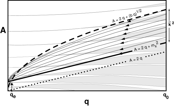
FIG. 1.: A sketch of the $(q,\,A)$ plane in which grey (white) strips represent instability (stability) regions of the Mathieu equation. The dotted line corresponds to $A=2q$. The thick solid line corresponds to $A=2q+m_{x}^{2}$, the trajectory of the $k=0$ mode (assuming $V(X)=0$). Also sketched (see thin solid lines with arrows) are trajectories with $k\leq\bar{k}$, which dominate the resonant amplification. Only trajectories lying below the dashed curve, $A=2q+\sqrt{bq}$ with $b={\cal O}(1)$, are significantly amplified; in the text, we explain how to use this curve to determine $\bar{k}$ and $q_{e}$.

FIG. 2.: Plot of $\rho_{x}/\rho_{total}$ vs. $m_{\phi}t/2\pi$ comparing numerical results (thin, ragged curves) to the heuristic Mathieu equation picture for various models (thick, smooth curves), where $2\pi/m_{\phi}$ is the inflaton oscillation period. The approximation reliably predicts the time-averaged behavior. The top pair of curves corresponds to the minimal $g$ required for the massless case to achieve efficient preheating, $\rho_{x}\approx\rho_{\phi}$. As predicted by the heuristic picture, increasing $m_{x}^{2}$ or $f(\chi)$ or decreasing $g$ greatly suppresses amplification.

FIG. 3.: A plot of $g$ vs. $m_{x}/m_{\phi}$ indicating the boundary between efficient preheating and inefficient preheating. Numerical results (circles) and the prediction based on the Mathieu equation (solid curve) are in good agreement. Note the lower bound on $g$ required to have efficient preheating, a bound which increases as $m_{x}$ increases.

FIG. 4.: For simplicity, the calculations in all three panels of the figure are done for a single $k=0$ mode of the $\chi$ field. Figure (a) shows the number of $\chi$-particles ($n_{\chi}$) produced as a function of time for a typical case of barely efficient preheating. Each time $\phi$ oscillates through its minimum, there is a sharp spike; however, particle production is measured by the time-averaged increase in $n_{x}$. Initially, when $q$ is large ($t/2\pi\leq 8$), the increases in $n_{x}$ occur in discrete jumps from one side of a spike to another. This behavior is just like the static Mathieu equation for high $q$, as shown in (b). At later times ($t/2\pi\geq 8$), the growth is continuous between spikes and across them, similar to the static Mathieu equation at small $q$, as shown in (c). For $t/2\pi\geq 12$, there are also rises and plateaus stretching many oscillations as $q$ spends many oscillations in one instability regime. In all cases, the figures show that the growth has an exponential envelope with exponent $\nu$ reliably predicted by the Mathieu picture.

REFERENCES

- [1] A. D. Linde, Phys. Lett. 108B, 389 (1982).
- [2] A. Albrecht and P. Steinhardt, Phys. Rev. Lett. 48, 1220 (1982).
- [3] A. Albrecht, P. Steinhardt, M. S. Turner, and F. Wilczek, Phys. Rev. Lett. 48, 1437 (1982).
- [4] A.D. Dolgov and A.D. Linde, Phys. Lett. 116B, 329 (1982).
- [5] L.F. Abbott, E. Farhi, and M. Wise, Phys. Lett. 117B, 29 (1982).
- [6] L. Kofman, A. Linde, and A. A. Starobinsky, Phys. Rev. Lett. 73, 3195 (1994).
- [7] D. Boyanovsky et al., Phys. Rev. D 51, 4419 (1995).
- [8] Y. Shtanov, J. Traschen, and R. Brandenberger, Phys. Rev. D 51, 5438 (1995).
- [9] L. Kofman, A. Linde, and A. A. Starobinsky, Phys. Rev. Lett. 76, 1011 (1996).
- [10] E. W. Kolb, A. Linde, and A. Riotto, Phys. Rev. Lett. 77, 4290 (1996).
- [11] S. Klebnikov and I. Tkachev, Phys. Rev. Lett. 77, 219 (1996).
- [12] S. Klebnikov and I. Tkachev, Phys. Lett. B390, 80 (1997).
- [13] H. Fujisaki, K. Kumekawa, M. Yamaguchi, and M. Yoshimura, Phys. Rev. D 54, 2494 (1996).
- [14] L. Kofman, A. Linde, and A. A. Starobinsky, hep-ph/9704452 (1997).
- [15] P. Greene, L. Kofman, A. Linde, and A. A. Starobinsky, hep-ph/9705347 (1997).
- [16] S. Klebnikov and I. Tkachev, hep-ph/9610477
- [17] S. Klebnikov and I. Tkachev, hep-ph/9701423
- [18] B. R. Greene, T. Procopec, and T. G. Roos, hep-ph/9705357 (1997).
- [19] R. Allahverdi and B. A. Campbelli, Phys. Lett. B390 , 169 (1997).
- [20] T. Procopec and T. G. Roos, Phys. Rev. D, 55, 3768 ( 1997).
- [21] A. Riotto and I. Tkachev, Phys. Lett. B385, 57 (1996).
- [22] N. W. McLachlan, Theory and Application of Mathieu Functions (Dover, New York, 1964).