Low Surface Brightness Radio Structure in the Field
of Gravitational Lens 0957+561

Abstract

We have produced deep radio maps of the double quasar 0957+561 from multiple-epoch VLA observations. To achieve high sensitivity to extended structure we have re-reduced the best available 1.6 GHz observations and have combined 5 GHz data from multiple array configurations. Regions of faint emission approximately 15″ north and south of the radio source G are probably lobes associated with the lensing galaxy. An arc 5″ to the east of G may be a stretched image of emission in the background quasar’s environment. 1.4″ southwest of G we detect a source that we interpret as an image of emission from the quasar’s western lobe, which could provide a constraint on the slope of the gravitational potential in the central region of the lens. We explore the consequences of these new constraints with simple lens models of the system.

1 Introduction

Astrophysicists have anticipated the use of gravitational lensing as an observational tool for 60 years (Zwicky (1937); Schneider, Ehlers, & Falco (1992)), and in the case of the double quasar 0957+561 (Walsh, Carswell, & Weymann (1979)), after 18 years of study the promise is closest to fulfillment. If one knew the details of the gravitational-lensing potential, and the time delay among the images of flux-variable components, one could make an estimate, albeit cosmology-dependent, of Hubble’s constant H₀ (Refsdal (1964)).

Efforts to measure the time delay in this system have converged recently (417$\pm$3, Kundić et al.  (1997); 420$\pm$13, Haarsma (1997)). However, models of the lensing potential have been less well constrained (Falco et al.  (1991); Kochanek (1991); Grogin & Narayan 1996a , 1996b) despite detailed observations of the cluster of galaxies providing the lensing mass (Young et al.  (1981); Angonin-Willaime, Soucail, & Vanderriest (1994); Fischer et al.  (1997)). In an effort to produce a definitive radio map of the object we undertook to re-reduce VLA data gathered by the M.I.T. group, discovering several new features in the field (Avruch et al.  (1993)). In this letter we present improved maps and identify features that may be useful as model constraints.

2 Observations

The data sets from which results presented in this letter were computed are listed in Table 1. We first mapped a low resolution $\lambda$6cm data set to identify any sources in the primary beam whose side lobes would contaminate the field of interest; during self-calibration of other data sets this emission was taken into account. For sensitivity to low surface brightness features we chose the best extant $\lambda$18cm observation. We have also combined five $\lambda$6cm data sets from array configurations A, B, and C to achieve more complete $(u,v)$ coverage and compensate for the reduced brightness at $\lambda$6cm compared to $\lambda$18cm. The fluxes of A and B were roughly constant at these epochs. Using the AIPS software, the data sets were independently mapped and self-calibrated following standard VLA reduction procedures (Fomalont & Perley (1989)). Each data set was phase self-calibrated several times, followed by a single amplitude self-calibration, provided that it reduced the map noise. The individual data sets were then co-added in AIPS and the combined data were mapped and self-calibrated as above. To produce source-subtracted images, we use the model for compact emission that the deconvolution algorithm creates in the form of CLEAN components, subtracting the model source from the visibility plane and remapping.

To the north and south of 0957+561 we have detected lobes of emission, separated by about 30″. The northern lobe (N) is more compact, with a $\lambda$6cm flux of about 840 $\mu$Jy and spectral index $\alpha^{\rm 18cm}_{\rm\phantom{string}6cm}\sim$ $-$1.0 ($S\propto\nu^{\alpha}$). The southern lobe (S) is extended, with a total flux of about 1000 $\mu$Jy, $\alpha^{\rm 18cm}_{\rm\phantom{string}6cm}\sim$ $-$0.7. These lobes may be associated with radio galaxy G, or with the lensed quasar in the background. To the east of the quasar images A and B we have detected an arc of emission (R1). The arc is clearly resolved tangentially, with a peak flux of 1.27 mJy beam^-1 at $\lambda$18cm and spectral index $\alpha^{\rm 18cm}_{\rm\phantom{string}6cm}\sim$ $-$0.8. In Figure 1 we present a radio map of these features; B has been subtracted from the image in the manner described above.

Galaxy G, the dominant contributor to the lensing potential, is definitely extended to the east, southwest, and northwest. To better view the structure near G, we subtracted from the multi-epoch $(u,v)$ data all emission associated with the B quasar image, the BN component (Roberts et al.  (1985)), and G. These structures were identified by directly inspecting the CLEAN components from the multi-epoch map. In Figure 2 the extension of G to the east we name GE, to the northwest GN, to the northeast GNE, and the brightest component of the arc-like structure to the southwest of G we call R2. Table 2 presents the positions and fluxes for these new components.

We are confident that these features are real. N, S, and R1 have been confirmed with detections by Harvanek et al.  (1996); R1 and perhaps GN have also been confirmed by Porcas et al.  (1996). The fainter features GE, GN, GNE, and R2 are visible in every individual, reduced data set with sufficient resolution and sensitivity, so it is unlikely that they are artifacts of calibration or deconvolution. On the other hand, detailed substructure such as the double peaks of GNE is not significant, because with extended sources CLEAN produces spurious peaks on that scale (Briggs (1995)).

3 Discussion

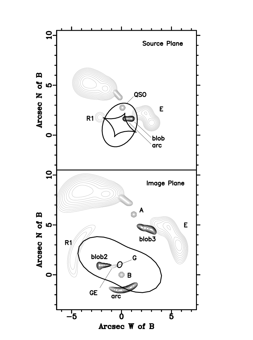
Figure 3: Lens model constrained to the HST components, showing disposition of radio components. The HST and radio components are shown as dark and light contours, respectively. The source plane shows how the source would appear without lensing; the caustics separate regions of multiple imaging. The image plane shows the model source seen through our lens model; the critical lines divide the images. The location of G is shown on the image plane, at the center of the lens model. Note that the HST arc is probably formed by the eastern end of the source that yields the HST blobs.

To illustrate our interpretation of these new VLA components, we used the LENSMOD software (Lehár et al.  (1993)) to model the lensing mass with a softened power-law potential (Blandford & Kochanek (1987)). The model parameters were: the lens position ($\Delta\alpha$, $\Delta\delta$), the critical radius ($b$), a core radius ($\theta_{c}$), the power index $P$ ($P=1$ is isothermal, while $P=2$ is a Hubble profile), the isodensity ellipticity ($e=1-\frac{\rm minor\;axis}{\rm major\;axis}$), and the major axis orientation ($\phi$). As constraints we used the new HST quasar and G1 positions (Bernstein et al.  (1997)) and required that the quasar images have a magnification ratio of 0.75$\pm$0.02 (Schild & Smith (1990)). We required that any third image of the quasar near G be at least 30 times fainter than B (as a 1$\sigma$ limit). We also added constraints from the new HST “blobs” and “arc.” We required that blob2 and blob3 be images of each other, and that the two knots in the arc share a common source. Note that the HST arc is probably caused by the eastern end of the same object that gives rise to blobs 2 and 3, and this could be used to further constrain lens models. To account for the possibility that the HST objects are at a different redshift than the quasar, we added a uniform scale factor $Q_{2}$ to the deflection angles for those components, as an extra model parameter. The lens model parameters were varied until the source plane position and magnitude differences for each pair were minimized, with a resultant reduced $\chi^{2}$ for the fit of 1.1. The best fit model parameters are given in Table 3, with uncertainties determined by varying the model parameters until the reduced $\chi^{2}$ increased by 1. Note that the $Q_{2}$ range corresponds to HST component redshifts of $z_{\rm HST}\approx 1.3\pm 0.1$ for an $\Omega=1$ cosmology, which is fully consistent with the quasar and HST objects being at the same redshift. Figure 3 shows the best fit model for $Q_{2}=1$, with components added to show the modeled radio emission. We do not attempt to account for the VLBI structures (Garrett et al.  (1994)) in this model, and thus make no claims about the time delay or Hubble’s constant based upon our model.

We interpret the component GE as the counter-image to the low surface brightness tail of the quasar’s western radio lobe E. GE’s peak surface brightness and spectral index ($\alpha^{\rm 18cm}_{\rm\phantom{string}6cm}\sim$ $-$1.0) matches that of component E’s northeastern extension, so the brighter parts of the lobe are not multiply imaged. The Bernstein et al.  (1996) HST blobs 2 and 3, almost certainly multiple images of a background object, are very close to the positions of GE and the northeast end of E; therefore we expect an image of E near where we have found GE. Because not all of E is multiply imaged, the detailed structure of GE can yield strong constraints on the central region of the lens: either the mass distribution is non-singular, in which case GE comprises two merging images of the eastern end of E, or, if the mass has a central singularity, GE will have a sharp cusp at its western end. High resolution radio observations of GE may be able to distinguish these two possibilities, or at least determine an upper limit on the size of the central mass concentration in G. This is also important because, for a given lens mass, the potential near the quasar B image is generally deeper for singular models, yielding a longer predicted time delay and thus a lower H₀ estimate.

The arc-like feature R1 may be a stretched image of background emission. As there is no clear counterpart to the west of G, it is unlikely to be multiply imaged. If the background source is circular, the axial ratio of R1 yields a lower limit of about 5 for its magnification. Jones et al. (1993), in Einstein HRI data, have detected an apparent x-ray arc about 3″ northwest of R1. The positions are formally consistent, but seem unlikely to be coincident judging from the relative positions of A and B. An association is not ruled out, however. The authors claim the extended x-ray source is an image of thermal emission from a cooling flow in the cluster hosting the lensed quasar at z = 1.41. There are examples of diffuse non-thermal radio emission associated with x-ray-emitting clusters (Deiss et al.  (1997)), and in this case the lensing magnification may have helped to make it observable. Of course this emission could be foreground; if G has radio lobes, N and S, it could as well have jets. R1 might be back flow from the lobe S, and GN might be a faint jet feeding the lobe N. GE is well explained as an image of the quasar’s E lobe, but it’s not impossible for it to be the counter-jet of GN, feeding lobe S.

The features R2, GN, and GNE are not readily explained by a lensing hypothesis. R2 is in the position of the western half of the HST arc, but all the models we have investigated would produce an eastward extension of this arc which is not detected. We could appeal, ad hoc, to source size and spectral index morphology causing the image to be unobservable. The component GN should have a brighter image 5″ south of G, which is not seen, though we could make the same appeal and note that it might be difficult to separate visually from S. GNE should also have a counter-image to the south of G, which is not seen. However, given the interpretation of R1 as lensed, and the faintness of these features, it is not ruled out that at least some of the emission is due to structure in the background quasar’s environment.

N and S are certainly not multiply imaged, but whether they are foreground or background is less clear. They could be the radio lobes of the galaxy G. At the lens redshift ($z=0.36$, and assuming $\Omega=1$, $h=0.75$) N and S would have a (projected) proper separation of 120 kpc, and luminosities at 178 MHz of about 10²⁴ WHz^-1, typical values for low power, limb darkened radio galaxies. The optical classification of G as a cD galaxy, and the fact that N and S are aligned within 30°  of its optical minor axis are also consistent (Miley (1980)). N and S might be old lobes of the background quasar, in which case the numbers are 170 kpc and 10²⁶WHz^-1, more appropriate for powerful, limb brightened sources. If N and S are associated with the quasar, the relatively small lobe separation (56 kpc) and the high core-to-lobe flux ratio ($R=0.22$) suggest that the jet axis is moderately inclined towards the line-of-sight (Muxlow & Garrington (1991)). This inclination readily explains the seemingly large rotation of the jet from the axis defined by N and S to that defined by C and E.

The performance of the VLA at $\lambda$18cm has improved markedly since 1980, and new observations should detect or exclude these features with high significance. We are aware of a very deep VLA observation (Harvanek et al.  (1996)) at $\lambda$18cm and $\lambda$3.6cm; the longer wavelength data should be able to confirm GE, GN, and GNE, and if GE is detected at $\lambda$3.6cm it may be possible to determine whether the mass model is singular, or whether GE consists of two merging images.

Figure 1: Contour plot of $\lambda$18cm A array map of 0957+561 on 1980 December 16. The cross hair marks the position at which the quasar B component has been subtracted from the map. The source just to the north of B is G, the lensing galaxy. Contour levels are $-$0.10%, 0.10%, 0.20%, 0.28%, 0.40%, 0.57%, 0.80%, 1.13%, 1.60%, 2.26%, 3.2%, 4.53%, 6.40%, 9.05%, 12.8%, 18.1%, 25.6%, 36.2%, and 51.2% of the peak intensity of 181 mJy beam^-1. The noise level is 105$\mu$Jy beam^-1. The box in the lower left shows the beam FWHM ellipse.

Figure 2: Contour plot of $\lambda$6cm map of 0957+561 from co-added observations in A, B, and C arrays (data sets #4 – #8, Table 1). The cross hairs ($+$) are the positions from which models of the components B (to the south) and G were subtracted. The crosses ($\times$) are, east to west, the positions of HST components “blob 2” and “blob 3.” The circles are positions along the HST arc, the outer two being the approximate extent and the inner two being “knot 1” and “knot 2.” Contour levels are $-$0.25%, 0.25%, 0.35%, 0.50%, 0.63%, 0.75%, 0.88%, 1.00%, 1.13%, 1.60%, 2.26%, 3.20%, 4.53%, 6.40%, 9.05%, 12.8%, and 51.2% of the peak intensity of 41.8 mJy beam^-1. The noise level is 39$\mu$Jy beam^-1. The box in the lower left shows the beam FWHM ellipse.

Table 1: Archival VLA Data Presented in this Letter.

No	Obs. Date	$\lambda$ (cm)	Duration (hrs)	VLA Config.
1	16DEC80	18	3.0	A
2	21AUG90	06	0.8	B
3	17MAR88	06	0.9	C
4	27SEP87	06	1.5	A
5	20JUL87	06	0.8	A
6	09DEC87	06	1.1	B
7	02JUN85	06	1.2	B
8	11JAN87	06	1.6	C

Table 2: Faint Emission Features Described in this Letter

Feature	($\Delta\alpha^{\arcsec}$,$\Delta\delta^{\arcsec}$)	$\lambda$6cm Peak	$\lambda$6cm Flux	$\lambda$18cm Flux
		mJy beam-1	mJy	mJy
N	($-$4.5string,string18.8string) $\pm$ (0.5string,0.5string)	0.440$\pm$0.053	0.840$\pm$0.110	10.15$\pm$0.66
S	(string1.5string,$-$11.7string) $\pm$ (0.5string,0.5string)	0.270$\pm$0.053	1.030$\pm$0.149	08.87$\pm$0.61
R1	(string5.38,string0.80) $\pm$ (0.59,1.17)	0.366$\pm$0.043	3.646$\pm$0.181	06.61$\pm$0.31
R2	($-$1.28,string$-$0.80) $\pm$ (0.26,0.21)	0.250$\pm$0.039	2.270$\pm$0.159	$\cdots$
GE	(string1.24,stringstring0.68) $\pm$ (0.04,0.04)	0.486$\pm$0.039	2.130$\pm$0.093	$\cdots$
GN	($-$0.24,string1.68) $\pm$ (0.12,0.24)	0.373$\pm$0.039	0.930$\pm$0.066	$\cdots$
GNE	(string2.24,string2.08) $\pm$ (0.34,0.22)	0.357$\pm$0.039	1.186$\pm$0.073	$\cdots$

Table 3: Best Fit Lens Model Parameters

Parameter	Best Fit Value
$\Delta\alpha$	$+$0$\farcs$181$\pm$0$\farcs$001
$\Delta\delta$	$+$1$\farcs$019$\pm$0$\farcs$001
$b$	string2$\farcs$88$\pm$0$\farcs$021
$\theta_{c}$	($<$0$\farcs$02)
$P$	0.88${}^{\rm+0.04}_{\rm-0.02}$
$e$	string0.538$\pm$0.018
$\phi$	$+$65.2$\pm$0.5string
$Q_{2}$	string1.03$\pm$0.02

References

- Angonin-Willaime, Soucail, & Vanderriest (1994) Angonin-Willaime, M.-C., Soucail, G., & Vanderriest, C. 1994, A&A, 291, 411
- Avruch et al. (1993) Avruch, I. M., Conner, S. R., Becker, D. J., & Burke, B. F. 1993, BAAS, 25, 1403
- Bernstein et al. (1997) Bernstein, G., Fischer, P., Tyson, J. A., & Rhee, G. 1997, ApJ, 483, L79
- Blandford & Kochanek (1987) Blandford, R. D., & Kochanek, C. S. 1987, ApJ, 321, 658
- Briggs (1995) Briggs, D. S. 1995, Ph.D. thesis, New Mexico Institute of Mining and Technology, Socorro
- Deiss et al. (1997) Deiss, B. M., Reich, W., Lesch, H., & Wielebinski, R. 1997, A&A, 321, 55
- Falco et al. (1991) Falco, E. E., Gorenstein, M. V., & Shapiro, I. I. 1991, ApJ, 372, 364
- Fischer et al. (1997) Fischer, P., Bernstein, G., Rhee, G., & Tyson, J. A. 1997, AJ, 113, 521
- Fomalont & Perley (1989) Fomalont, E. B., & Perley, R. A. 1989, in ASP Conference Series, Vol. 6, Synthesis Imaging in Radio Astronomy, ed. R. A. Perley, F. R. Schwab, & A. H. Bridle (San Francisco: Astronomical Society of the Pacific), 83
- Garrett et al. (1994) Garrett, M. A., Calder, R. J., Porcas, R. W., King, L. J., Walsh, D., & Wilkinson, P. N. 1994, MNRAS, 270, 457
- (11) Grogin, N. A. & Narayan, R. 1996, ApJ, 464, 92
- (12) Grogin, N. A. & Narayan, R. 1996, ApJ, 473, 570
- Haarsma (1997) Haarsma, D., B. 1997, Ph.D. thesis, M.I.T., Cambridge
- Harvanek et al. (1996) Harvanek, M., Stocke, J., Tyson, T., & Rhee, G. 1996, BAAS, 28, 843
- Jones et al. (1993) Jones, C., Stern, C., Falco, E., Forman, W., David, L., & Shapiro, I. 1993, ApJ, 410, 21
- Kochanek (1991) Kochanek, C. S. 1991, ApJ, 382, 58
- Kundić et al. (1997) Kundić, T., et al. 1997, ApJ, 482, 75
- Lehár et al. (1993) Lehár, J., Langston, G. I., Silber, A., Lawrence, C. R., & Burke, B. F. 1993, AJ, 105, 847
- Miley (1980) Miley, G. 1980, in ARA&A, Vol. 18, ed. G. Burbidge, D. Layzer, & J. G. Phillips (Palo Alto: Annual Review Inc.), 165
- Muxlow & Garrington (1991) Muxlow, T. W. B., & Garrington, S. T. 1991, in Beams and Jets in Astrophysics, ed. P. A. Hughes (New York: Cambridge University Press), 52
- Porcas et al. (1996) Porcas, R. W., Patnaik, A. R., Muxlow, T. W. B., Garrett, M. A., Walsh, D. 1996, in Astrophysical Applications of Gravitational Lensing, ed. C. S. Kochanek & J. N. Hewitt (Boston: Kluwer Academic Publishers), 349
- Refsdal (1964) Refsdal, S. 1964, MNRAS, 128, 307
- Roberts et al. (1985) Roberts, D. H., Greenfield, P. E., Hewitt, J. N., Burke, B. F., & Dupree, A. K. 1985, ApJ, 293, 356
- Schild & Smith (1990) Schild, R. E., & Smith, R. C. 1990, AJ, 101, 813
- Schneider, Ehlers, & Falco (1992) Schneider, P., Ehlers, J., & Falco, E. E., 1992 Gravitational Lenses (New York: Springer-Verlag)
- Walsh, Carswell, & Weymann (1979) Walsh, D., Carswell, R. F., & Weymann, R. J. 1979, Nature, 279, 381
- Young et al. (1981) Young, P., Gunn, J. E., Kristian, J., Oke, J.B., & Westphal, J. A. 1981, ApJ, 244, 736
- Zwicky (1937) Zwicky, F. 1937, Phys. Rev., 51, 290