An improved technique of image analysis for IACTs and IACT Systems

Abstract

In order to better utilize the information contained in the shower images generated by imaging Cherenkov telescopes (IACTs) equipped with cameras with small pixels, images are fit to a parametrization of image shapes gained from Monte Carlo simulations, treating the shower direction, impact point, and energy as free parameters. Monte Carlo studies for a system of IACTs predict an improvement of order 1.5 in the angular resolution. The fitting technique can also be applied to single-telescope images; simulations indicate that the shower direction in space can be reconstructed event-by-event with a resolution of $0.16^{\circ}$ to $0.20^{\circ}$, allowing to generate genuine source maps. Data from Crab observations with a single HEGRA telescope confirm this prediction.

1 Introduction

Over the last decade, imaging atmospheric Cherenkov telescopes have proven the prime instrument for $\gamma$-ray astronomy in the TeV domain [1]. Both the orientation and the shape of Cherenkov images are exploited to supress cosmic-ray background in the search for point sources of $\gamma$ rays: $\gamma$ shower images seen in the camera point back to the source location, and are characterized by narrow, compact images. In contrast, cosmic rays generate hadronic showers with wider and more diffuse images, and random orientation.

Recent improvements of the imaging Cherenkov technique include the use “high-resolution” cameras with pixel sizes of $0.15^{\circ}$ or less, capable of resolving fine details of the image, and the stereoscopic technique, where a shower is observed simultaneously by several telescopes, allowing to geometrically reconstruct the shower axis, and hence the direction of the primary particle. Since Cherenkov shower images in the camera point to the image of the source, the apparent source of air shower can be reconstructed by superimposing the images of several cameras and intersecting the image axes (Fig. 1) [2, 3, 4].

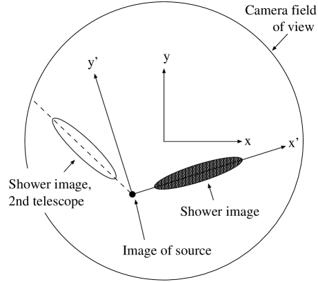
Figure 1: Image of a shower in the camera, with the coordinate system $(x,y)$ fixed to the camera, and the system $(x^{\prime},y^{\prime})$ defined by the source image and the direction to the shower impact point (after accounting for the reversal of signs occuring for the mirror image). Also illustrated is the reconstruction of the shower direction using images from multiple telescopes.

Opposite to the source image, the shower image points towards the location where the shower axis intersects the plane of the telescope dish. The impact location can be therefore be derived by extrapolating the image axes, starting from the locations of the telescopes, until the lines intersect at one point .

Cherenkov images are traditionally described by parameters related to the first and second moments of the intensity distribution in the camera [5]: the center of gravity, the length of the major and minor axis of the image “tensor of inertia”, and its orientation. While rather powerful, this method has two shortcomings: it does not make use of the full information obtained with todays cameras, where a typical shower lights up twenty and more pixels, and it requires the use of a “tail cut” to eliminate pixels which do not belong to the image, yet show some signal due to night-sky background light. Since this tail cut is usually set at a level around 5 photoelectrons, tails of the image are excluded, too.

To provide tools for an improved image analysis, we have, over the last years, developed a technique [6, 7] which makes better use of the information contained in the image, by fitting the observed intensities to a model of Cherenkov images, with the showers characteristics - direction, core location, and energy - as free parameters. In this paper, we describe first the simulation and parametrization of the images, then the fitting procedure and its predicted performance when used in a system of imaging Cherenkov telescopes. Finally, we apply the fitting technique also to single-telescope data and demonstrate its performance using images obtained with one of the HEGRA Cherenkov telescopes during observations of the Crab Nebula. Emphasis on the present work is on this interpretation of single-telescope images; multi-telescope data has become available, but the analysis is still in the early stages [3].

A similar reconstruction technique has been studied by the CAT group [8].

2 Modeling of Cherenkov images

To perform a fit of the intensity profile of Cherenkov images, an analytical parametrization of images was derived on the basis of Monte Carlo simulations. The relevant parameters of the shower are its impact distance $R$ from the telescope, the shower energy $E$, the zenith angle $\Theta$ of the shower, and, to a certain extent, the height $h_{max}$ of the shower maximum. Other shower parameters, such as the orientation of the shower axis, or the direction towards the location of the shower core, correspond simply to translations and rotations of the image; images are hence described in a coordinate system $(x^{\prime},y^{\prime})$ with its origin at the image of the source, and the $x^{\prime}$-axis pointing towards the shower impact point in the plane defined by the telescope dish (see Fig. 1) . Neglecting for the moment the $h_{max}$-dependence, the photoelectron density in the image is given by a function $\rho(x^{\prime},y^{\prime}|R,E,\Theta)$, which in the following will be factored into a longitudinal profile and a transverse profile, $\rho(x^{\prime},y^{\prime})=\rho_{L}(x^{\prime})\rho_{T}(y^{\prime}|x^{\prime})$, with $\int\rho_{T}(y^{\prime}|x^{\prime})dy^{\prime}\equiv 1$.

The parametrization refers to a camera with infinite granularity; to compare with an actual image, the parametrized images are shifted and rotated according to the presumed shower orientation, and the image intensity is integrated over the area of each of the camera pixels. Since image shapes vary slowly with shower energy, the simulation effort was simplified by generating events at one typical energy $E_{0}$, and scaling the intensities afterwards according to energy. Similarly, the dependence on the zenith angle was introduced in a simplified fashion: only vertical showers ($\Theta=\Theta_{0}=0$) were considered, and image sizes (for fixed $R$) were later scaled with $\cos\Theta$, reflecting the increasing distance of showers from the camera for larger $\Theta$. Since most analyses so far concentrated on small zenith angles (less than $30^{\circ}$), this assumption works sufficiently well.

2.1 Simulation of Cherenkov images

The simulation code [9, 10] tracks electromagnetic and hadron-induced cascades and includes the propagation of Cherenkov light in the atmosphere, and the wavelength-dependent characteristics of the telescopes, such as reflectivity of the mirrors, the efficiency of the light collectors in front of the PMTs, and the PMT quantum efficiency. Image intensities and image characteristics have been compared with other simulation codes, and good agreement has been found [11]. The simulations use the characteristics of the HEGRA telescopes [12, 13], in particular the mirror area of 8.5 m² and the location at of 2200 m a.s.l. To parametrize the images, 10000 vertical showers were generated and observed with telescopes positioned at 15 distances between 0 and 300 m from the shower axis. In case of $\gamma$ ray initiated showers, a fixed energy $E_{0}=1$ TeV was chosen. For studies concerning hadron rejection, also proton showers were generated; here, $E_{0}=3$ TeV was used, resulting in roughly the same number of photoelectrons in a typical image.

2.2 Longitudinal image profile

The longitudinal image profile $\rho_{L}(x^{\prime}|R,E_{0},\Theta_{0})=\rho_{L}(x^{\prime}|R)$ is obtained by projecting the image onto the $x^{\prime}$ axis, and averaging over many showers. We note that the coordinate $x^{\prime}$ measures essentially the height of emission $h$ of a photon, $x^{\prime}\approx R/h$, up to effects caused by the finite radial extent of the shower. Comparing the profiles of individual showers with the average profile (for a given $R$), one notices that the average profile does not describe the individual images very well; they tend to be narrower. The explanation is simply that the height of the shower maximum, and hence the location of the peak of the longitudinal profile fluctuates from shower to shower. The typical rms variation of one radiation length in the height $h_{max}$ of the shower maximum translates into a variation in $x^{\prime}$ of about 15% (for a typical height of the shower maximum of 6 km above ground). Since a parametrization is needed which applies to individual rather than average images, the height of the shower maximum of each simulated shower was determined from the evolution of the number of shower particles with depth, and all images were scaled to the same average height of the shower maximum, before averaging over the individual longitudinal profiles. In the fits of Cherenkov images for multi-telescope observations, the height $h_{max}$ was correspondingly included as a free parameter, which manifests itself as a scale factor for the image sizes. Since for stereoscopic shower observations the impact point is strongly constrained by the geometrical relations discussed earlier, both the impact point and the height of the shower maximum can be determined separately. Fig. 2 shows the resulting longitudinal profiles for different impact distances.

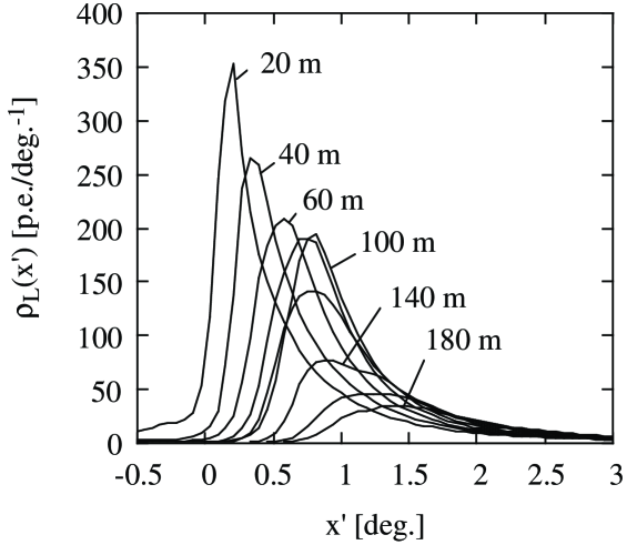
Figure 2: Longitudinal image profile for 1 TeV $\gamma$-ray showers at different distances $R$ = 20,40,60,80,100,120,140,160,180 m between shower axis and telescope, as determined from Monte-Carlo simulations.

We note that this type of parametrization has one disadvantage: in some distance ranges, a peak or shoulder in the angular distribution of photons at the typical Cherenkov angle reflects emission in the early stages of the shower, where the smearing of angular distributions due to multiple scattering of shower particles is small; due to the rescaling of angles, this structure is smeared out.

To describe the longitudinal profile as a function of $x^{\prime}$ and $R$, a two-dimensional spline function was fit [14] to the simulation data, with the number and location of node points (19x17) optimized to obtain a sufficiently good representation.

2.3 Transverse image profile

The transverse width of the Cherenkov image largely reflects the width of the shower disk, or equivalently the angular distribution of shower particles. One therefore sees a very narrow image at small values of $x^{\prime}$, corresponding to large heights, and a wide image at large values of $x^{\prime}$, corresponding to the tail of the shower. Samples of transverse profiles are shown in Fig. 3.

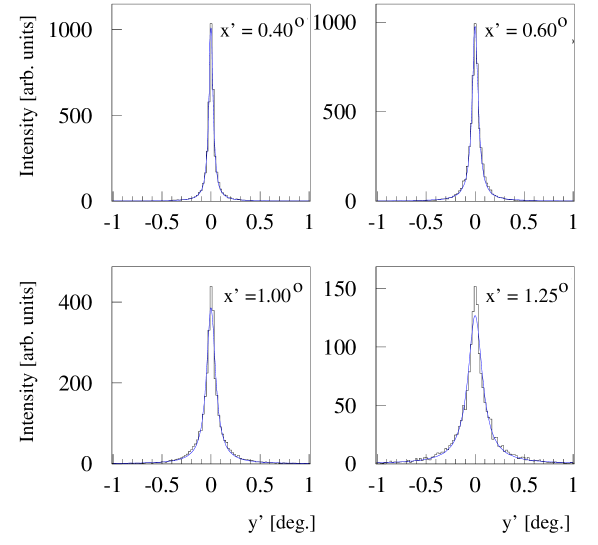
Figure 3: Transverse image profiles for $R=60$ m and different values of $x^{\prime}$, as obtained from Monte-Carlo simulations, together with the fit function.

For all distances $R$ and relevant values $x^{\prime}$, the transverse profile $\rho_{T}(y^{\prime}|x^{\prime},R)$ is well described by the one-parameter function

$$\rho_{T}(y^{\prime}|x^{\prime},R)={1\over\pi}{w(x^{\prime},R)\over y^{\prime 2}+w^{2}(x^{\prime},R)}$$

where the width of the profile is characterized by $w$. Fig. 4 illustrates how $w$ varies with $x^{\prime}$, for two different shower distances $R$. We note the pronounced asymmetry in the image with respect to its center of gravity along $x^{\prime}$, both in the longitudinal profile, and in the width of the transverse profile. This asymmetry is ignored in the conventional second-moment image parameters. An interesting observation is that the shape of the transverse image profile illustrates why tail cuts are absolutely necessary in the second moment image analysis, even in the absence of night-sky background: with a profile varying like $1/y^{\prime 2}$ for large $y^{\prime}$, the second moment does not converge without some kind of cutoff, either in amplitude or directly in $y^{\prime}$!

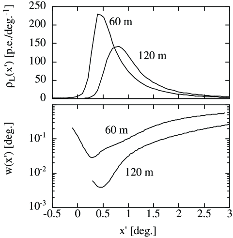
Figure 4: Width parameter $w(x^{\prime},R)$ of the transverse distribution as a function of the longitudinal coordinate $x^{\prime}$, for core distances $R$ of 60 m and 120 m. For reference, the corresponding longitudinal distributions $\rho_{L}(x^{\prime}|R)$ are also shown.

For use in the image fits, the width $w(x^{\prime},R)$ is again described by a two-dimensional spline function.

2.4 Fluctuations of image intensitities

In order to properly fit Cherenkov images and to obtain error estimates for the shower parameters, it is not sufficient to provide a parametrization of image profiles as a function of the relevant parameters, one needs also to know the fluctuations of the intensities measured in the individual pixels of the camera. With the fit based on a $\chi^{2}$ minimization, strictly speaking one needs the covariance matrix of the amplitudes in all pixels. In particular, longitudinal profiles of electromagnetic showers in matter are known to exhibit large correlated fluctuations; the energy deposition in nearby sections shows a positive correlation, whereas the energy deposition in early and late slices of showers is anticorrelated. Most of this correlation, however, can be traced simply to the fluctuation in the location of the shower maximum; once this effect is removed, correlations are modest. The dependence of longitudinal profiles on the shower maximum is however already explicitly taken into account in our model, by treating it as a free parameter in the fit. We therefore considered the pixel amplitudes as independent, and included in the errors a term describing the Poisson fluctuation in the number, a term accounting for PMT gain fluctations (using a width of the single-photoelectron peak of about 70%), and a term accounting for night-sky background and electronics noise (about one photoelectron in case of the HEGRA telescopes).

3 Fitting of Cherenkov images

The fitting technique to derive shower parameters was initially developped to be used for system of Cherenkov telescopes; more recently, it was successfully applied to images from single telescopes. In this chapter, we briefly summarize the technique and the simulation studies carried out for the HEGRA system of Cherenkov telescopes.

3.1 Fit procedure

Shower parameters are optimized to best describe the measured images by numerically minimizing the $\chi^{2}$ function

$$\chi^{2}=\sum_{j}\sum_{i}w_{i,j}{\left(a_{i,j}-(E/E_{0})\int_{\mbox{pixel}}\rho(x^{\prime},y^{\prime})dx^{\prime}dy^{\prime}\right)}^{2}~{}~{}~{}.$$

Here, $a_{i,j}$ is the amplitude measure in the $i$-th pixel of the $j$-th camera, and the weight $w_{i,j}$ is calculated based on the expected fluctuation of pixel amplitudes, $w_{i,j}=1/\sigma^{2}_{i,j}$. The predicted amplitudes are obtained by integrating the intensity profile over the pixel area. The minimization and the error estimates for the fit parameters are carried out with standard routines [14], treating the shower direction (2 parameters), the impact point (2 parameters), the energy, and the height of the shower maximum as free parameters.

In order to achieve rapid convergence of the fit, the choice of good starting values is essential. For the shower direction and impact point, the starting values were derived using a conventional geometrical reconstruction. In cases where only two telescopes contribute, direction and impact point are directly given by the intersections of the image center lines; for events with more telescopes, the shower parameters were determined separately from each pair of telescopes, and averaged, weighted with the sine of the angle between the views. Given these starting values, and the assumed linear dependence between light yield and energy, a starting value for the energy $E$ can be derived analytically. The average height of the shower maximum is used to seed the height of the shower maximum.

Since the integration over pixel area is partly numerical and time-consuming, the number of pixels included in the determination of $\chi^{2}$ was limited to those containing potentially relevant information, plus a boundary region. These boundary pixels should contain no signal, but are required to ensure the stability of the fit . Typically, all pixels were included which were within an ellipse with half-axes equal to 5 times the width and length Hillas image parameters; for events with very small width or length, a fixed region was used.

3.2 Fitting of multi-telescope images

The simulation studies were carried out for a system similar to the HEGRA CT system [12, 13] under installation on the Canary Island of La Palma, at the Observatorio del Roque de los Muchachos of the Instituto Astrofisico de Canarias. The telescopes are located at 2200 m a.s.l., have 8.5 m² mirror area and are equipped with 271-pixel cameras, with a pixel size of $0.25^{\circ}$ and a hexagonal field of view of $4.3^{\circ}$ effective diameter. Four telescopes form the corners of a square with about 100 m sides, the fifth telescope is located in the center of the square. The simulations used PMT quantum efficiencies measured for an earlier generation of PMTs; the actual PMTs used are about 30% more efficient and hence thresholds should be scaled down correspondingly. The simulation implemented a trigger condition close to one used in HEGRA: at least two pixels of a camera need to detect 10 or more photoelectrons to fire the telescope trigger, and at least two telescopes need to trigger to accept the event. Two modes of analysis were considered. In one mode, only telescopes which had triggered were included in the analysis; in the other mode, also telescopes which did not trigger, but had images with at least 20 photoelectrons were included (the HEGRA telescopes with their Flash-ADC readout system and signal storage allow to recover the signal even if a telescope did not trigger). In the following, resolutions for the shower direction and the impact position are given for both modes. The resolutions quoted correspond to the diameter of a circle containing 68% of the events.

Fig. 5 displays the angular resolution of the telescope system as a function of energy, both for fitting technique (a) and the conventional geometrical reconstruction (b). One notices a significant improvement if the image fit is used. In particular at small energies, adding non-triggered telescopes improves the fit further. A surprising feature is that the angular resolution worsens for large energies, particularly dramatic in case of the conventional reconstruction. The reason is that showers at increasingly larger distances contribute, and hence the stereo angles under which the telescopes view the shower decrease, correspondingly increasing the reconstruction errors. If only showers with impact points within 120 m from the center of the system are included, the angular resolution improves to better than $0.05^{\circ}$ at 10 TeV in case of the fit. Fig. 5(c),(d) shows the resolution in the reconstruction of the shower impact point; again, the fit provides a clear improvement over the simple geometrical reconstruction. A good localization of the impact point is important to allow reliable energy estimates. The height of the shower maximum is reconstructed with an rms error of 0.9 radiation lengths; the energy resolution is typically 20% to 25%, almost independent of the energy of the incident photon.

Figure 5: Resolution in the reconstruction of the shower direction (a),(b) and of the shower impact position (c),(d) using a five-telescope system, shown as a function of energy. The resolution is defined such that 68% of all events are contained within a circle of the given diameter. The resolutions are shown both using the fitting technique (a),(c), and the conventional image analysis (b),(d). Open symbols: only triggered telescopes included in the analysis (2 pixels above 10 photoelectrons). Full symbols: also including non-triggered telescopes with at least 20 photoelectrons in the image.

Overall, the fitting technique provides an improvement in resolution by typically a factor 1.5, and up to 2 in special regimes.

3.3 $\gamma$-hadron separation using the image fit

We had initially hoped that the fitting technique would also provide significant improvements in the $\gamma$-hadron separation based on image shapes (as opposed to image orientation). Various techniques were tried, such as cuts on the quality ($\chi^{2}$) of the fit with the $\gamma$-shower parametrization, or the fit of images with both a $\gamma$-shower model and an analoguous proton shower model, and cuts applied to the absolute $\chi^{2}$ as well as to the $\chi^{2}$ difference between the two fits. To judge the quality of a scheme, the enhancement in the signal-to-noise ratio was used, $\epsilon_{\gamma}/\sqrt{\epsilon_{CR}}$. While the various techniques did improve the signal-to-noise of $\gamma$-signals, none of the variants was clearly superior to the classical image cuts, which typically select $\gamma$-candidates as events with small width and length, a large concentration of the signal in a few pixels, and possibly a small amount of clutter outside the main image cluster. It appears that the remaining correlations between pixels and the non-gaussian signal fluctuations hurt the fit in this respect, and are more effectively captured by the classical global event variables. Since the classical variables are much faster to calculate, we have in most applications and studies pre-selected the $\gamma$-candidates based on the normal shape parameters, and then applied the fit to best reconstruct the shower parameters, i.e. the direction, impact point, and energy.

4 Shower reconstruction for single-telescope images

For Cherenkov observations with a single imaging telescope, the location of the source, i.e. the direction of the primary, is constraint to lie on the image axis (see Fig. 1). However, its position along this axis is not fixed. For this reason, Cherenkov telescopes do usually not provide images corresponding to those of optical telescopes, where a source shows up as a peak in a two-dimensional map. Rather, a location of a source is assumed, and it is checked if there is an excess of events consistent with this source location.

To remedy this situation, it is tempting to apply the image fit to single-telescope images. The shape (length) of the image does contain information about the impact distance $R$, and hence about the distance between the peak of the Cherenkov image and the image of the source (see Fig. 2). The pronounced asymmetry of the image along $x^{\prime}$ allows to distinguish on which side of the image the source is likely to be located. The image fit should be able to extract this information in an optimum fashion. In addition, it provides an improved reconstruction of the image axis and accounts for image distortions caused by the outer edge of the camera, which tend to severely distort conventional image parameters once images approach the camera border.

Applied to a single image, the fit cannot distinguish well between the influence of the impact distance $R$, and variations in the height of the shower maximum $h_{max}$, since to first order the image depends only on $h_{max}/R$. Therefore, in our single-telescope fits, the height of the shower maximum was frozen. As starting values for the shower parameters, a source location separated from the center of gravity of the image by 3 times the image length along the image axis was used. There is a two-fold ambiguity in the choice of the starting value. We usually chose the point closer to the center of the camera, but also tried a variant where the fit was performed for both starting values, and the best fit was chosen as the final result.

Monte-Carlo studies were again carried out for telescopes of the HEGRA type, this time with a trigger condition requiring two pixels above 15 photoelectrons, as required for single-telescope running in order to limit noise triggers. The simulation showed that IACT images contain indeed enough information to estimate the impact parameter of the shower and hence the distance between the center of the shower image, and the image of the source, with useful accuracy. In the $x^{\prime}$ direction - along the image axis - the fit reconstructs the shower direction with a resolution between $0.13^{\circ}$ and $0.17^{\circ}$, depending somewhat on the criteria for event selection. The resolutions quoted are obtained from a gaussian fit to the $x^{\prime}$-distribution of reconstructed shower axes. The resolution in the transverse ($y^{\prime}$) direction is significantly better, around $0.08^{\circ}$ to $0.09^{\circ}$. Alternatively, one can quote a resolution in space, defined as the radius of a circle containing 68% of the reconstructed events. The resulting values range between $0.17^{\circ}$ and $0.23^{\circ}$ and are slightly larger than expected based on the Gaussian widths in $x^{\prime}$ and $y^{\prime}$, indicating slight non-Gaussian tails in the resolution function. The fit provides an average energy resolution of 22%.

At first sight, it may seem surprising that the resolution in $x^{\prime}$ is only a factor two worse than the resolution in $y^{\prime}$ (which corresponds to the width of the distribution of the conventional miss parameter). However, it does not even require the admittedly not very transparent fitting procedure to extract the information on the distance $d$ between the center of the image, and the image of the source. Among the conventional image parameters, the ratio of width over length of the image shows an almost linear depedence on $d$ and can be used to estimate $d$ with an rms precision of about $0.25^{\circ}$ (see also, e.g., [15]). The use of the ratio of the width and length parameters has the advantage that the strong dependence of the individual parameters on the image amplitude cancels to a large extent. Third moments of the longitudinal image profile can be used to distiguish the ‘head’ and ‘tail’ of the shower with reasonable reliability, i.e. allow to resolve the two-fold ambiguity in the source location. In this sense, the fitting procedure actually provides more of a quantitative rather than a qualitative improvement of the image analysis. Nevertheless, the extraction of the shower direction from single-telescope images represents a significant step, and it was felt that such a claim should not be supported by simulation studies alone. The analysis was therefore applied to data gained in observations of the Crab Nebula with the HEGRA telescope CT3, the first of the HEGRA telescopes to be equipped with a 271-pixel camera [13].

4.1 Application to single-telescope Crab data

The Crab data set used here comprises 80 h of observations, equally distributed between on-source and off-source runs, resulting in a total of $1.2\cdot 10^{6}$ events at zenith angles below $45^{\circ}$. This data set shows a clear signal for TeV $\gamma$-ray emission ([3], Fig. 1).

Because of an initial lack of readout channels of some of the pixels near the fringe of the camera, analyses of this data set were mostly restricted to the central 169 pixels. Events were collected with a trigger condition requiring two pixels with signals above 15 photoelectrons. In a first analysis step, events were preselected on the basis of the conventional second-moment image parameters. The cuts included a distance cut at $1.1^{\circ}$ or $1.3^{\circ}$ to exclude heavily truncated images, and the requirements width $<~{}0.13^{\circ}$, $0.15^{\circ}~{}<$ length $<~{}0.35^{\circ}$, and concentration $>~{}0.4$. The selection reduced the sample by a factor 6. In the next step, the images were fit. No further cuts on the fit quality were applied, since the preselected images showed acceptable values of $\chi^{2}$ of the fit, and on the basis of Monte-Carlo studies no further improvement in $\gamma$-ray selection was expected. Fig. 6(a) shows the distribution of the reconstructed shower directions for the Crab data sample, after subtraction of the off-source data set. A clear excess at the center of the camera, at the location of the Crab Nebula, is evident, with a characteristic width of about $0.2^{\circ}$. This ‘true’ source image from one of the HEGRA Cherenkov telescopes nicely demonstrates the power of the fitting technique.

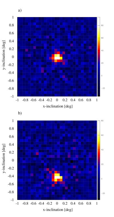
Figure 6: (a) Distribution of the direction of fitted $\gamma$-ray showers relative to the direction to the Crab Nebula (located at the center of the camera), after subtraction of the off-source sample. (b) Same sample, but reconstructed using a “shifted” camera, in which the Crab Nebula is $0.42^{\circ}$ off-center.

While it is unlikely that an artefact in the reconstruction procedure generates such a narrow spike, the center of the camera is nevertheless a preferred location and one would like to demonstrate that the technique works equally well for off-center sources. Lacking data with the Crab off-center, we made use of the fact that the camera is actually larger than the 169 pixels used in this analysis, and selected another set of pixels shifted by about $0.42^{\circ}$ with respect to the center of the camera (see Fig. 7).

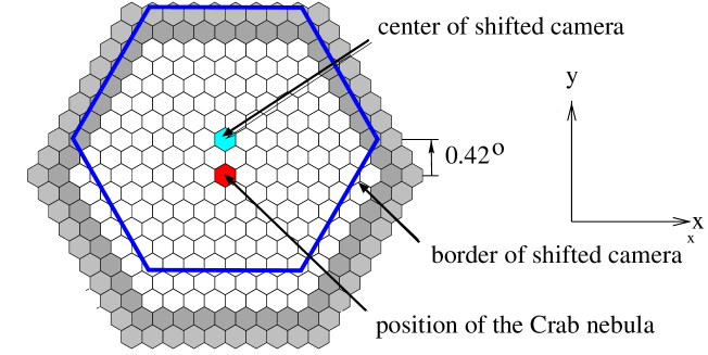
Figure 7: Camera of HEGRA telescope CT3, showing the 169 pixels used in the initial Crab analysis (the shaded two outer rings were excluded), and the second set of 169 pixels shifted with respect to the center of the camera.

The image analysis was then repeated with this “new” camera, with distance cuts etc. applied relative to the new center. The result is shown in Fig. 6(b); an excess of events is seen which is shifted by $0.42^{\circ}\pm 0.01^{\circ}$ with respect to the new camera center, as expected. The width of the peak is within errors identical with the original peak. This test demonstrates that the method is able to properly reconstruct off-center sources.

From the width of the Crab signal, the angular resolution can be determined. Projecting the excess on the $x$ or $y$ axis, one finds that the distributions are within statistics described by Gaussians with a width of $0.10^{\circ}\pm 0.01^{\circ}$ to $0.11^{\circ}\pm 0.01^{\circ}$, depending on the distance cut in the pre-selection. While the width of the excess is, within errors, identical in $x$ and $y$, the simulations predict that on an event-by-event basis the reconstruction of the shower direction works better in the $y^{\prime}$ direction, perpendicular to the image axis, than in the $x^{\prime}$ direction parallel to the image axis, where the image shape has to be used to estimate the impact distance. Fig. 8 shows the distribution of the excess along $x^{\prime}$ and $y^{\prime}$, confirming this expectation. The corresponding angular resolutions are summarized in Table 1, both for the data and the simulations, for two choices of the distance cut applied to select events. Within errors, the measured angular widths agree with the simulation results.

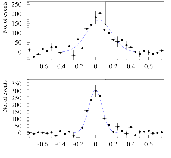
Figure 8: Distribution of the Crab signal in the directions $x^{\prime}$ (along the image axis) and $y^{\prime}$ (perpendicular to the image axis), after background subtraction on the basis of off-source runs. The curves represent gaussian fits.

	Data	Monte Carlo
Distance $<1.1^{\circ}$
Average $(x,y)$	$0.10^{\circ}\pm 0.01^{\circ}$	$0.102^{\circ}$
Longitudinal $(x^{\prime})$	$0.14^{\circ}\pm 0.02^{\circ}$	$0.133^{\circ}$
Transverse $(y^{\prime})$	$0.08^{\circ}\pm 0.01^{\circ}$	$0.086^{\circ}$
Distance $<1.3^{\circ}$
Average $(x,y)$	$0.11^{\circ}\pm 0.01^{\circ}$	$0.112^{\circ}$
Longitudinal $(x^{\prime})$	$0.15^{\circ}\pm 0.02^{\circ}$	$0.165^{\circ}$
Transverse $(y^{\prime})$	$0.08^{\circ}\pm 0.01^{\circ}$	$0.084^{\circ}$

Table 1: Angular resultions obtained from the Crab data set, compared to Monte-Carlo simulations. The resolutions quoted are derived from a Gaussian fit to the distribution of reconstructed shower axes, projected onto the $(x,y)$ or $(x^{\prime},y^{\prime})$ directions (see Fig. 1). For the Monte Carlo data sets, statistical errors are $0.002^{\circ}$ or less.

Due to the improved angular resolution of the fit, and the (at least partial) resolution of head-tail ambiguities, one should expect a corresponding increase in the significance of signals from point sources. The Monte-Carlo studies show that, compared to conventional analyses, the number of background events $N_{BG}$ after cuts is reduced by a factor 2. Since also some of the signal events are misreconstructed and lost, the significance, which is governed by $N_{S}/\sqrt{N_{BG}}$, is predicted to increase by typically 30%, rather than by a full factor $\sqrt{2}$. In the Crab data, the background reduction is indeed observed as predicted. The improvement in the significance of the excess, however, amounts only to about 15%, due to an increased loss of signal events. Given the limited statistics of the Crab data set, the origin of this difference between data and simulation could not be resolved.

5 Outlook

The analysis presented in this paper emphasizes two points

• Modern imaging cameras provide more information on image details, than are exploited by the second-moment image analysis. Detailed models of the light distribution can be used to extract additional information, and to improve the reconstruction of the image parameters, in particular concerning the direction of the primary particle. Angular resolutions can be improved by factors 1.5 to 2.

• While conceived for the analysis of stereoscopic observations of air showers with multiple telescopes, the technique can also be applied to single-telescope data, where it provides the option to generate a genuine source map, rather than testing the hypothesis of a source at one specific location. Using the relation between the shower impact parameter and the length and width of an image, this technique to construct source maps can also be employed in simplified form, based only on the second-moment image parameters, at some expense in resolution.

References

References

- [1] T.C. Weekes, Space Science Rev. 75 (1996) 1; M. F. Cawley and T.C.Weekes, Experimental Astronomy 6 (1996) 7.
- [2] A. Kohnle et al., Astroparticle Physics 5 (1996) 119.
- [3] A. Daum et al., Preprint astro-ph/9704098 (1997), Astroparticle Phys., in press.
- [4] C.W. Akerlof et al., Astrophys. J. 377 (1991) L97.
- [5] A.M. Hillas, Proc. 19th ICRC, La Jolla, Vol. 3 (1985) 445.
- [6] M. Ulrich, Proceedings of the Int. Workshop “Towards a Major Atmospheric Cherenkov Detector IV”, Padua, (1995), M. Cresti (Ed.), p. 121.
- [7] M. Ulrich, Ph.D. Thesis, Heidelberg (1996).
- [8] S. Le Bohec, Proceedings of the Int. Workshop “Towards a Major Atmospheric Cherenkov Detector IV”, Padua, (1995), M. Cresti (Ed.), p. 378.
- [9] A. Plyasheshnikov, A. Konopelko, K. Vorobiev, Preprint 92 P N, Lebedev Physical Institute (1988).
- [10] A. Konopelko, A. Plyasheshnikov, A. Schmidt, Preprint 6 P N, Lebedev Physical Institute (1992).
- [11] F. Aharonian et al., Astroparticle Phys. 6 (1997) 343.
- [12] F. Aharonian, Proceedings of the Int. Workshop “Towards a Major Atmospheric Cherenkov Detector II”, Calgary, (1993), R.C. Lamb (Ed.), p. 81.
- [13] G. Hermann, Proceedings of the Int. Workshop “Towards a Major Atmospheric Cherenkov Detector IV”, Padua, (1995), M. Cresti (Ed.), p. 396.
- [14] NAG Fortran Library, The Numerical Algorithms Group, Oxford, 1990.
- [15] P.J. Boyle et al., astro-ph/97061132 (1997)