Measuring non-axisymmetry in spiral galaxies

Abstract

We present a method for measuring small deviations from axisymmetry of the potential of a filled gas disk. The method is based on a higher order harmonic expansion of the full velocity field of the disk. This expansion is made by first fitting a tilted–ring model to the velocity field of the gas disk and subsequently expanding the velocity field along each ring into its harmonic terms. We use epicycle theory to derive equations for the harmonic terms in a distorted potential. The phase of each component of the distortion can vary with radius. We show that if the potential has a distortion of harmonic number $m$, the velocity field as seen on the sky exhibits an $m-1$ and $m+1$ distortion. As is to be expected, the effects of a global elongation of the halo are similar to an $m=2$ spiral arm. The main difference is that the phase of the spiral arm can vary with radius. Our method allows a measurement of $\epsilon_{\rm pot}\sin 2\varphi_{2}$, where $\epsilon_{\rm pot}$ is the elongation of the potential and $\varphi_{2}$ is one of the viewing angles. The advantage of this method over previous approaches to measure the elongations of disk galaxies is that, by using H i data, one can probe the potential at radii beyond the stellar disk, into the regime where dark matter is thought to be the dominant dynamical component. The method is applied to the spiral galaxies NGC 2403 and NGC 3198 and the harmonic terms are measured up to ninth order.

The residual velocity field of NGC 2403 shows some spiral-like structures. The harmonic analysis indicates that the $m=3$ term is dominant, with an average value of $\sim 0.02v_{c}$. This is consistent with an average ellipticity of the potential of $\epsilon_{\rm pot}\sin 2\varphi_{2}=0.064\pm 0.003$, but spiral arms may couple significantly to this result.

In the harmonic analysis of the kinematics of NGC 3198 the $m=2$ and $m=3$ terms are strongest ($\sim 0.01v_{c}$). The inferred average elongation of the potential is $0.019\pm 0.003$. Since the amplitude of the elongation is coupled to the viewing angles and may be influenced by spiral arms, more galaxies should be examined to separate these effects from true elongation in a statistical way.

1 Introduction

It is generally accepted that disk galaxies have massive dark halos but little is known about their shape. Dark halos were generally modeled as being spherical until Binney (1978) proposed that the natural shape of dark halos is triaxial in order to explain warped disks. Triaxial dark matter halos occur naturally in cosmological N-body simulations of structure formation in the universe. These simulations also indicate that there may well be a universal density profile for dark matter halos (Navarro, Frenk & White 1996; Cole & Lacey 1996), but the exact distribution of halo shapes is as yet uncertain (Katz & Gunn 1991; Dubinski & Carlberg 1991; Warren et al. 1992; Dubinski 1994). The main problem is numerical resolution, but the inclusion of baryons is also important. If baryons are included, the baryonic disk that forms in the centre of the dark matter distribution tends to make the halo more oblate (Barnes 1994; Dubinski 1994). So the observed distribution of the shapes of dark matter halos can be a constraint on scenarios of galaxy formation and subsequent galaxy evolution. Measuring the shapes of dark halos can be split in two parts: measurement of the ratio $c/a$, i.e., flattening perpendicular to the plane of the disk, and measurement of the intermediate to major axis ratio $b/a$, i.e., elongation in the plane of the disk. Polar ring galaxies provide clues on the axis ratio $c/a$, by comparing the rotation curve of the disk with the rotation of the inclined ring. Unfortunately, the values found for $c/a$ are not unique, since the interpretation of the data is model dependent, but all measurements now seem to be consistent with $c/a<1$ (Whitmore, McElroy, Schweizer 1987; Sackett & Sparke 1990; Sackett et al. 1994). For our own galaxy, van der Marel (1991, and references therein) tried to determine the flattening of the galactic halo using counts and kinematics of halo stars. He found that the axis ratio of the galactic dark halo must satisfy $c/a>0.34$. Finally, measurements of the flaring of the H i disks of spiral galaxies may give us a direct handle on the flattening of the dark halo of normal spiral galaxies. Olling (1995a) developed a method to measure $c/a$ using gas flaring, and found a very high flattening of $c/a=0.1-0.5$ for the nearly edge-on galaxy NGC 4244 [Olling 1995b]. Preliminary results from Sicking (1997), who developed a method for measuring the thickness of inclined gas disks, indicate $0.2<c/a<0.8$ for NGC 3198 with a best value of $0.5$, whereas the measurements for NGC 2403 are difficult and give no conclusive value for the flattening of the dark halo. From these measurements, it seems that spherical halos can indeed be excluded, although no good value for the typical flattening of a dark halo has been found yet.

The elongation of the dark halo ($b/a$) is an even more undetermined parameter. A few attempts have been made to determine the typical elongation of disk galaxies on either photometric or kinematic basis. On the basis of a large sample (13,482) of spiral galaxies from the APM survey, Lambas et al. (1992) find that a pure oblate model of spiral galaxies does not fit the observations and $b/a\sim 0.9$ fits best, consistent with the findings of Binney & de Vaucouleurs (1981). However, Lambas et al. remark that this effect may also be due to the presence of spiral arms and bars in the disks. On the basis of a distance-limited sample of 766 spiral galaxies, Fasano et al (1992) also conclude that spiral galaxies cannot be oblate, although early type spirals seem to have more triaxial disks than their late type spirals. Furthermore, their late type spiral group falls into two parts: those without bars seem to be consistent with oblate shapes, whereas those with bars are not. These two effects may suggest that a triaxial bulge or bar might be responsible for the observed triaxiality, although an intrinsic elongation cannot be ruled out by these observations.

More detailed imaging of a small sample of spiral galaxies can give a better handle on the effects of spiral arms and bars. For this purpose, imaging of the old stellar population in the $\mbox{K}^{\prime}(2.2\mu)$ band was done by Rix & Zaritsky (1995). They observed a sample of 18 spiral galaxies and found a variety of asymmetries in this sample. They estimated the potential in the plane of the disk to have an average ellipticity of $0.045^{+0.03}_{-0.02}$, but remarked that this number may only be an upper limit to the true ellipticity, since spiral structure still couples significantly to their estimated ellipticity.

A second way to examine elongation of the potential of disk galaxies, is to look at the kinematics of the disks. For our own galaxy, Kuijken & Tremaine (1994) find on the basis of solar neighbourhood kinematics plus kinematics of a more global kind (H i tangent point velocities, Cepheids, etc) that our sun lies near the minor axis of the slightly elongated ($b/a\sim 0.9$) Milky Way disk. Franx & de Zeeuw (1992) used the scatter in the Tully-Fisher relation to place limits on the elongation of spiral disks, since elongation will increase the scatter. Based on the observed scatter alone, they find that $b/a>0.9$, but they argue that it is unlikely that the scatter is caused solely by elongation and therefore the value is on average likely to be $b/a>0.94$.

The only direct measurement of the elongation of the potential of a disk galaxy so far comes from the S0 galaxy IC 2006 (Franx, van Gorkom & de Zeeuw 1994, hereafter FvGdZ), which contains a large H i ring in the plane of the disk. Using information on both the kinematics and the geometry of the ring, FvGdZ were able to measure the elongation of the potential at the place of the ring. The measured elongation is consistent with zero. FvGdZ used epicyclic theory to determine the geometry and velocity field of a ring in a mildly perturbed potential. If the ring is in an elongated potential, the velocity variation along the ring will not be pure circular rotation, but higher harmonic terms will be superposed on it. Making a harmonic expansion of the velocity field of the ring and interpreting the measured harmonics within the framework of epicycle theory, given the ring geometry, allows the elongation of the potential at the position of the ring to be found. In this paper, we extend the method used in FvGdZ for a single ring to the case of a filled gas disk in order to study individual halo elongations for a larger sample of spiral galaxies.

With a single ring, one has the advantage that the ring can be considered as a single orbit. Therefore, one knows for each point in the ring to which orbit it belongs. We will lose this advantage in the case of a filled gas disk. Since galactic disks are not obviously made out of separate rings, we will decompose the H i disks of spiral galaxies into individual rings (the so-called tilted–ring method, Begeman 1987) and perform a harmonic expansion on each of these rings (Binney 1978; Teuben 1991; FvGdZ). The harmonic expansion can be done to arbitrary order and it produces amplitudes and phases for each separate order. We will investigate if we can qualitatively distinguish between the effects of spiral arms and of elongation on the velocity field. We will apply this method to two spiral galaxies with extended H i disks, NGC 2403 and NGC 3198. From the measurements of these galaxies, the strengths and limitations of our method will become clear. We will see that in both cases contributions of spiral arms to the velocity field are important, but that nevertheless limits to the halo elongation can be set.

The outline of this paper is as follows: In Section 2 we lay down the theoretical framework for connecting the measured kinematic terms to perturbations of the potential. We describe the resulting procedure to fit observed velocity fields in Section 3. In Section 4 we present some examples of the theory, to see what effects may play a role in interpreting the measured harmonics. Next, we examine two spiral galaxies: NGC 2403 in Section 5 and NGC 3198 in Section 6. We conclude with a discussion on the results from these galaxies. In the Appendix, we give a detailed derivation of the equations presented in Section 2. Furthermore, we derive what the effect of misfitting ring parameters (inclination, position angle and centre) is on the measured harmonics.

2 Description of a perturbed velocity field

2.1 General perturbations

If the cold H i gas in a disk galaxy orbits in the potential of an axisymmetric dark halo, the resulting density field and velocity field are axisymmetric as well. This means that the velocity field will only show pure circular rotation. Observed velocity fields of disk galaxies generally can indeed be fitted quite accurately by circular motion. Many different effects can cause the remaining small residuals. Here, we will analyse the case of a small distortion in the potential $V$, which can be written as a sum of harmonic components, each of which may have a different pattern speed. This is not the most general description possible, as it does not include non-stationary phenomena such as spiral arms. But it is a good description for the motion of gas in a triaxial halo, since the potential distortion, i.e., the elongation of the halo, can be considered stationary. Furthermore, we will assume that the gas moves in a symmetry plane on stable closed orbits. This assumption cannot be correct in detail, since this description of the gas motion does not allow for shocks in the gas and therefore cannot give an accurate description of spiral arms. On the other hand, this is a correct assumption if we are interested in the motion of gas in a nearly circular potential [Tohline, Simonson & Caldwell, 1982], like the potential of a mildly elongated halo. Although these assumptions restrict the validity of our description, it will help us to gain some understanding of the qualitative characteristics of velocity fields.

Figure 1: Geometry of the projected orbit. The line $(\theta_{\rm obs},i)$ is the line-of sight. The inclination $i$ is measured from the $z$-axis, the axis perpendicular to the plane of the orbit. The angle $\theta_{\rm obs}$ is measured from the line $\theta=0$ and the azimuthal angle $\psi$ is measured in the plane of the orbit and is zero at the line of nodes, which is indicated by the dashed line.

The assumptions that the potential contains a small stationary distortion and that the gas moves on stable closed orbits allow us to use epicycle theory to analyse the velocity fields that originate from such a perturbed potential. We will solve the equations of motion in this perturbed potential for the possible closed orbits and calculate the velocity field of these orbits as it would be seen by an external observer. In this way we can directly relate the observed velocity field to the potential of disk galaxies.

Let $R$ and $\theta$ be polar coordinates in the rest frame of the galaxy under consideration and consider a rotating, non-axisymmetric potential in that frame. The potential can be written as:

$$V(R,\theta,t)=V_{0}(R)+\sum_{m}V_{m}(R)\cos\{m[\theta-\Omega_{p,m}t-\phi_{m}(R)]\}.$$ (1)

Here, $V_{0}(R)$ represents the unperturbed potential and $V_{m}(R)\cos\{m[\theta-\Omega_{p,m}t-\phi_{m}(R)]\}$ is the m-th harmonic component of the perturbation, assumed to be small compared to $V_{0}(R)$. The phase of the perturbation as a function of radius is denoted as $\phi_{m}(R)$. Each of the harmonic components is allowed to have its own pattern speed, $\Omega_{p,m}$. If the perturbation has non-zero pattern speed, or $\phi_{m}(R)$ is not constant as a function of radius, then the choice of the line $\theta=0$ is arbitrary. We focus on the velocity field as generated by a potential perturbed by a single harmonic component. The general case, equation (1), can be obtained by adding the results for individual harmonic components, since coupling terms between different harmonic components are of second order. For a single harmonic component, the potential in a frame that corotates with the potential perturbation can be written as

$$V(R,\phi)=V_{0}(R)+V_{m}(R)\cos\{m[\phi-\phi_{m}(R)]\},$$ (2)

where $\phi=\theta-\Omega_{p,m}t$. The procedure we follow to find the closed orbits in this potential is analogous to the procedure followed by Binney & Tremaine (1987, eq. 3-107 and further), where they derive orbits in a potential with arbitrary $m$, but without the radially dependent phase we introduce here. We solve the equations of motion for a potential perturbed by a single harmonic component in Appendix A.1 and find the set of possible closed loop orbits for any value of $m$. Let us denote the solutions of the equations of motion in the unperturbed potential $V_{0}(R)$ that represent circular orbits by $R_{0}$ and $\phi_{0}$. If we then perturb the potential with a single harmonic component as indicated above, we find the set of closed loop orbits, equation (16):

$$R(\phi,t)\!\!\! = \!\!\!R_{0}\left(1-\textstyle{1\over 2}a_{1m}\cos\eta_{m}-a_{2m}\sin\eta_{m}\right),$$

$$\phi(R,t)\!\!\! = \!\!\!\phi_{0}(t)+\textstyle{1\over 2m}(a_{1m}+a_{3m})\sin\eta_{m}-a_{4m}\cos\eta_{m},$$ (3)

where $\eta_{m}=\eta_{m}(R,t)=m[\phi(t)-\phi_{m}(R)]\approx m[\phi_{0}(t)-\phi_{m}(R)]=m\{[\Omega_{0}(R)-\Omega_{p,m}]t-\phi_{m}(R)\}$ and $\Omega_{0}(R)$ is the usual circular frequency. The amplitudes $a_{xm}$ are defined in equations (A.1) of the Appendix.

The resulting velocity field in the non-rotating frame for a general rotation curve is

$$v_{R}\!\! = \!\!mv_{c}(R)[1-\omega(R)]\left(\textstyle{1\over 2}a_{1m}\sin\eta_{m}-a_{2m}\cos\eta_{m}\right),$$

$$v_{\phi}\!\! = \!\!v_{c}(R)\left\{1+\textstyle{1\over 2}[(1-\omega)a_{3m}+(\alpha-\omega)a_{1m}]\cos\eta_{m}\right.$$

$$\left.\phantom{\textstyle{1\over 2}}+[m(1-\omega)a_{4m}-(1-\alpha)a_{2m}]\sin\eta_{m}\right\},$$

where $\omega(R)\equiv{\Omega_{p,m}/\Omega_{0}(R)}$ and $v_{c}(R)=R\Omega_{0}(R)$, the circular velocity. We have defined $\alpha={d\ln[v_{c}(R)]}/{d\ln R}$. This velocity field is observed from a direction $(\theta_{\rm obs},i)$, where $i$ is the inclination of the disk and $\theta_{\rm obs}$ is defined as the angle between the line $\theta=0$ and the observer, see Figure 1.

Introduce $\psi=\theta-\theta_{\rm obs}+\pi/2=\phi-\phi_{\rm obs}+\pi/2$, where $\phi_{\rm obs}$ is the angle in the rotating frame that corresponds to $\theta_{\rm obs}$. The angle $\psi$ is measured along the orbit and is zero on the line of nodes. It is sometimes called the azimuthal angle. It is defined fully by the orientation of the galaxy on the sky and it is independent of the internal coordinate system. It is straightforward to derive that the velocity field of a disk in pure circular rotation is given by $v_{\rm los}=v_{c}(R)\sin i\cos\psi$.

Let us express the line-of-sight velocity as $v_{\rm los}=\sum_{n}c_{n}\cos n\psi+s_{n}\sin n\psi$. In Appendix A1 we show that the line-of-sight velocity field has the following form:

$$v_{\rm los}\!\! = \!\!\left[c_{1}\cos\psi+s_{m-1}\sin(m\!-\!1)\psi+c_{m-1}\cos(m\!-\!1)\psi\right.$$ (5)

$$\left.+s_{m+1}\sin(m\!+\!1)\psi+c_{m+1}\cos(m\!+\!1)\psi\right],$$

where

$$c_{1} = v_{*}$$

$$s_{m-1} = v_{*}(-\textstyle{\frac{1}{4}}\{[m\!-\!(m\!+\!1)\omega_{m}+\alpha]a_{1m}$$

$$+(1\!-\!\omega_{m})a_{3m}\}\sin m\varphi_{m}\textstyle{+\frac{1}{2}}\left\{m(1\!-\!\omega_{m})a_{4m}\right.$$

$$\left.+[m(1\!-\!\omega_{m})-1+\alpha]a_{2m}\right\}\cos m\varphi_{m}),$$

$$c_{m-1} = v_{*}(\textstyle{\frac{1}{4}}\{[m\!-\!(m\!+\!1)\omega_{m}+\alpha]a_{1m}$$

$$+(1\!-\!\omega_{m})a_{3m}\}\cos m\varphi_{m}\textstyle{+\frac{1}{2}}\left\{m(1\!-\!\omega_{m})a_{4m}\right.$$

$$\left.+[m(1\!-\!\omega_{m})-1+\alpha]a_{2m}\right\}\sin m\varphi_{m}),$$

$$s_{m+1} = v_{*}(\textstyle{\frac{1}{4}}\{[m\!-\!(m\!-\!1)\omega_{m}-\alpha]a_{1m}$$

$$-\!(1\!-\!\omega_{m})a_{3m}\}\sin m\varphi_{m}\textstyle{+\frac{1}{2}}\left\{m(1\!-\!\omega_{m})a_{4m}\right.$$

$$\left.-[m(1\!-\!\omega_{m})+1-\alpha]a_{2m}\right\}\cos m\varphi_{m}),$$

$$c_{m+1} = v_{*}(-\textstyle{\frac{1}{4}}\{[m\!-\!(m\!-\!1)\omega_{m}-\alpha]a_{1m}$$

$$-(1\!-\!\omega_{m})a_{3m}\}\cos m\varphi_{m}\textstyle{+\frac{1}{2}}\left\{m(1\!-\!\omega)a_{4m}\right.$$

$$\left.-[m(1\!-\!\omega)+1-\alpha]a_{2m}\right\}\sin m\varphi_{m}),$$

and we have written $v_{*}=v_{c}\sin i$ and $\varphi_{m}=\phi_{\rm obs}-{\pi}/{2}-\phi_{m}(R)$. Now we have expressed all observable parameters in terms of internal parameters for a potential perturbed by a single harmonic term.

From equation (5) we can conclude that if the potential has a perturbation of harmonic number $m$, the line-of-sight velocity field contains an $m-1$ and $m+1$ harmonic term. Qualitatively, this conclusion was also inferred by Canzian (1993). Furthermore, we can see from the definitions of the $a_{xm}$ in the Appendix, that the amplitudes of the $m-1$ and $m+1$ terms behave in the following way: if $\Omega_{0}>\Omega_{b}$, the $m-1$ term is larger in amplitude than the $m+1$ term. If $\Omega_{0}<\Omega_{b}$, the situation is reversed.

In general, we do not a priori know the inclination $i$ (or $q=\cos i$), position angle $\Gamma$ and centre $(x,y)$ of the galaxy. Here, the position angle $\Gamma$ is defined as the angle taken in anti-clockwise direction between the north direction on the sky and the direction of the major axis of the receding half of the galaxy. Usually, it is assumed that the velocity field is circular, and the values of the inclination and position angle are derived from the best fit. If the true velocity field contains non-circular terms this procedure will produce wrong values of $i$ and $\Gamma$ and of the position of the centre. If the velocity field is expanded on the basis of these incorrect viewing angles and centre, the harmonic terms will change. In Appendix A2 we derive the effect of errors in these parameters: $\delta q=\delta\cos i$, $\delta\Gamma$ and centre $\delta x,\delta y$. Under these incorrect parameters the line-of-sight velocity becomes:

$$v_{\rm los}\!\!\! = \!\!\!v_{*}(\hat{R})\left\{(1+\alpha){\delta x\over 2R}-(1-\alpha){\delta q\over 4q}\cos\hat{\psi}\right.$$

$$\!\!\!\!\!\!\!\!\!\!\left.-{\delta\Gamma\over 4}\left[(3q+{1\over q})-\alpha({1\over q}\!-\!q)\right]\sin\hat{\psi}\!\!-\!\!(1\!-\!\alpha){\delta x\over 2R}\cos 2\hat{\psi}\right.$$

$$\!\!\!\!\!\!\!\!\!\!\left.-(1-\alpha){\delta y\over 2qR}\sin 2\hat{\psi}+(1-\alpha){\delta q\over 4q}\cos 3\hat{\psi}\right.$$

$$\!\!\!\!\!\!\!\!\!\!\left.-(1-\alpha){\delta\Gamma\over 4}({1\over q}-q)\sin 3\hat{\psi}\right\}+$$

$$\!\!\!\!\!\!\!\!\!\!+\sum_{i\geq 0}c_{i}(\hat{R})\cos i\hat{\psi}+s_{i}(\hat{R})\sin i\hat{\psi}.$$

where $\hat{\psi}$ the angle in the plane of the ring that is zero on the apparent major axis of the ring and the $s_{i},c_{i}$ etc. are defined as in equation (2.1).

The harmonics arising from an $m=2$ term will mix with the terms caused by a misfit of the viewing angles. Since the tilted-ring algorithm has no way to disentangle the effects of a misfit of the viewing angles from that of a physical $m=2$ term, there will be first order differences between the best fitting and true ring parameters for $m=2$, see Appendix (A3.2). The same is true for an $m=1$ term and the centre, Appendix (A3.1). Also, an $m=4$ term will cause $c_{3},s_{3}$ terms, as shown in equation (5). Due to these terms, the position angle and inclination will change as well according to equation (2.1), creating new $\hat{c}_{1},\hat{s}_{1},\hat{c}_{3},\hat{s}_{3}$ terms. This affects the measurement of the elongation of the potential and is an extra source of noise on our measurement. In the same way, an $m=3$ term can cause similar effects as an $m=1$ term. For $m>4$, the harmonics in equation (5) do not change to first order due to small errors in the inferred viewing angles and centre.

2.2 Global elongation

We now turn to the case of a globally elongated potential, as caused by for instance a triaxial halo. In this case we have $m=2$, $\omega\approx 0$ and $\phi_{2}(R)\sim\mbox{const}$ (see also Appendix A.3.2). We will assume a flat rotation curve ($\alpha=0$), since rotation curves in the outer parts of galaxies where the dark matter halo dominates are basically flat. Furthermore, as rotation curve shapes approach solid body rotation ($\alpha=1$), the errors in the tilted ring fits become large (see Appendix 3.3) and a reliable determination of the elongation is no longer possible. In the flat rotation curve case, the relation between the measured $a_{12}$ and the ellipticity of the potential $\epsilon_{\rm pot}$ is $a_{12}=\epsilon_{\rm pot}$ and $a_{32}=2\epsilon_{pot}$ (FvGdZ).

The measured line-of-sight velocity along each ring in the velocity field will have the following form, as derived by FvGdZ (note that their equations for $c_{1}$ and $s_{1}$ contain typesetting errors):

$$v_{\rm los}=\hat{c}_{1}\cos\hat{\psi}+\hat{s}_{1}\sin\hat{\psi}+\hat{s}_{3}\sin 3\hat{\psi},$$ (8)

with

$$\hat{c}_{1} = v_{*}[1+\epsilon_{\rm pot}\cos 2\varphi_{2}],$$

$$\hat{s}_{1} = -v_{*}{(1-q^{2})^{2}\over{2(1+2q^{2}+5q^{4})}}\epsilon_{\rm pot}\sin 2\varphi_{2},$$

$$\hat{c}_{3} = 0,$$ (9)

$$\hat{s}_{3} = v_{*}{(1-q^{2})(1+3q^{2})\over{2(1+2q^{2}+5q^{4})}}\epsilon_{\rm pot}\sin 2\varphi_{2},$$

From the $\hat{c}_{1}$, $\hat{s}_{1}$ and $\hat{s}_{3}$ terms we can derive $\epsilon_{\rm pot}\sin 2\varphi_{2}$. This is the quantity that we will be looking for in our measurements of spiral galaxies.

Unfortunately, we cannot measure $\varphi_{2}$ separately (the $\cos 2\varphi_{2}$ term cannot be measured, since we do not know the exact value of $v_{*}$), so all we can measure is the combination of viewing angle and ellipticity. Global ellipticity will thus result in $s_{1}$ and $s_{3}$ terms that are constant with radius (and thus $\epsilon_{\rm pot}\sin 2\varphi_{2}$ will be constant as a function of radius as well), whereas spiral arms will cause $s_{1}$ and $s_{3}$ terms that change sign as a function of radius and $\epsilon_{\rm pot}\sin 2\varphi_{2}$ will wiggle, as we shall see in Section 4. Radial variation in $\epsilon_{\rm pot}\sin 2\varphi_{2}$ may help us to distinguish between the effects of spiral arms and systematic elongation.

Equation (2.2) shows that the $c_{3}$ term should always be zero. If the inclination is not equal to the best fitting inclination, the $c_{3}$ terms will not be equal to zero. Therefore, monitoring $c_{3}$ in the fitting procedure will be a useful way to check the correctness of the fitted inclination. Furthermore, spiral arms will also influence the measurements of the inclination. As shown in the Appendix, if $\varphi_{2}(R)$ is constant, the fitted inclination for each ring is identical to the true inclination for that ring. But, if $\varphi_{2}(R)$ varies as a function of radius, the fitted inclination will deviate from the true inclination. This effect will not be large (typically one or two degrees), but it will be measurable.

3 Fitting velocity fields

3.1 The method

In order to determine the variation of different harmonic components as a function of radius, we want to fit the velocity field of a galaxy along individual, independent rings. Within the GIPSY package (Groningen Image Processing SYstem, van der Hulst et al., 1992) there is a routine that fits a set of so-called tilted–rings to the velocity field of a galaxy. The code fits a circular model to the velocity field by adjusting the ring parameters (kinematic centre $(x_{0},y_{0})$, inclination $i$, position angle $\Gamma$ and systemic velocity $v_{\rm sys}$), so we have a list of ring parameters as a function of radius. All the ring parameters are simultaneously fitted with a general least-squares fitting routine. In the tilted–ring fit, we should take a uniform weighting function since points near the minor axis contain information about ellipticity. It is best to keep the centre fixed in the fit because the galaxy may contain physical $c_{2},s_{2}$ harmonics in its velocity field. In that case, a free centre would drift in such a way as to make these terms disappear. If a galaxy would be truly lop-sided in its kinematics (i.e., the kinematic centre drifts as a function of radius), this would show itself in the $c_{2}$ and $s_{2}$ terms, as can be seen from equation (38).

After the tilted ring decomposition we make a harmonic expansion of the radial velocity along each ring (using the ring’s individual $\Gamma,i,x_{0},y_{0}$):

$$v_{\rm los}=v_{\rm sys}+\sum_{n=1}^{k}\hat{c}_{n}\cos n\hat{\psi}+\hat{s}_{n}\sin n\hat{\psi},$$ (10)

where $k$ is the order of the fit. The coefficients $\hat{c}_{n},\hat{s}_{n}$ are determined by making a least-squares fit with a basis

$$\left\{1,\cos\hat{\psi},\sin\hat{\psi},\cdots,\cos k\hat{\psi},\sin k\hat{\psi}\right\},$$ (11)

on the data points in each ring.

We assume here that we can identify each pixel in the velocity map with a unique position in the galaxy. Strong warps in the outer H i -layers for instance tend to invalidate this assumption, since the value of the velocity field in a certain pixel may be composed of two or more rings (the line-of-sight crosses 2 or more rings) and the velocity field will not be accurate there. Mild warping where the viewing angles change by only a few degrees will in general not be a problem, as long as individual rings do not overlap each other.

3.2 Error estimates

The errors given by the tilted–ring decomposition code and by the harmonic fitting procedure are formal errors of the fits and do not take correlation between points due to beam smearing into account. Sicking (1997) has derived that the formal errors should be multiplied by a factor

$$\beta=\sqrt{4\pi\sigma_{x}\sigma_{y}\over{\delta x\delta y}},$$ (12)

where $\delta x,\delta y$ are the dimensions of a pixel in arcsec and $\sigma_{x},\sigma_{y}$ are the dispersions of the beam in arcsec. All measurement errors presented in this paper are corrected for this correlation effect.

4 Some example velocity fields

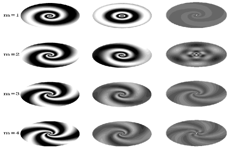
Figure 2: Potential perturbations and decomposed velocity fields. From top to bottom: the $m=1,2,3$ and 4 terms, from left to right : a. The potential perturbation, b. the residual velocity field (total velocity field minus circular velocity), showing mainly the $m-1$ component. No tilted-ring fit had to be made to find the circular velocity, since the circular velocity is a known input paramenter in these models. c. The residual field minus the $m-1$ component, revealing the $m+1$ component. To find this component a harmonic fit has been made. Normally, when creating residual fields, one would also subtract the kinematic $m=0$ term. In that case, the kinematic $m=0$ term in the top row, middle column, would be zero and one would only see the kinematic $m=2$ term. If the centre would be a free parameter in the tilted–ring fit, any kinematic $m=2$ component in the residual field would be zero as well. Finally, the alternating behaviour of the $m=3$ kinematic term (second row, third column) is due to the fact that in the tilted–ring fit the inclination is a free parameter. Therefore, the $c_{3}$ term is fitted to zero and only the $s_{3}$ term is visible.All plots are on the same scale. The potential ranges from $-80$ km² s^-2 to $80$ km² s^-2 , all velocity components from $-2$ km s^-1 to $2$ km s^-1. White denotes positive, black negative values.

In order to clarify the equations presented in Section 2 and in Appendix A, we present some example velocity fields in Figure 2. The different terms range from $m=1$ to $m=4$. For the phase of the fields, $\varphi_{m}(R)$, we chose a logarithmic spiral, $\varphi_{m}(R)=\ln({R}/{R_{\rm s}})/\tan p$. The amplitude of the perturbation has been taken constant throughout the field. In Table 1, we summarise the parameters used to create the model fields. The fields are then created using equations (5) and (2.1). Subsequently, these line-of-sight velocity fields were fitted as described in Section 3, revealing the two harmonic components that were hidden in them.

The example velocity fields are shown in Figure 2. We display from left to right

1. The potential containing the $m$ term perturbation.

2. The residual velocity field caused by this potential perturbation (i.e., the $m-1$ plus $m+1$ terms together).

3. The $m+1$ component of the velocity field.

Table 1: Parameters used for model fields

quantity	symbol	value
inclination	i	60°
obs. angle	$\phi_{\rm obs}$	$45\degr$
pattern speed	$\Omega_{p,m}$	0 km s-1 kpc-1
amplitude	$V_{m}$	80 km2 s2
circular velocity	$v_{c}$	150 km s-1
maximum radius	$R_{max}$	18 kpc
spiral scale length	$R_{s}$	10 kpc
pitch angle	p	$10\degr$

We see that indeed an $m$ term in the density causes $m-1$ and $m+1$ terms in the kinematics of the gas. Since the pattern speed $\Omega_{p}$ was taken zero for all models, the $m-1$ term will be dominant, see Section 2. The $m=2$ potential perturbation demonstrates the effect of fitting a circular model to a non-circular velocity field. The fitting procedure adapts the inclination until $c_{3}=0$ so that only the $s_{3}$ term remains. In our example, the $s_{3}$ term varies as a function of radius. If the field would have contained a global intrinsic ellipticity, $m=2,\varphi_{2}(R)=\mbox{const}$, the $s_{1}$ and $s_{3}$ terms would have been constant as a function of radius. Therefore, the measured $s_{3}$ would have been constant and non-zero as well, but no radially alternating pattern for $s_{3}$ would have been visible.

Since in the fitting procedure the centre was kept fixed, we also see a two-armed spiral in the $m=1$ case. If we would have taken the centre as a free parameter in the fit, it would have drifted in such a way as to make the $c_{2}$ and $s_{2}$ terms disappear.

We shall encounter the effects discussed above again while interpreting the data of NGC 2403 and NGC 3198.

5 NGC 2403

5.1 Data description

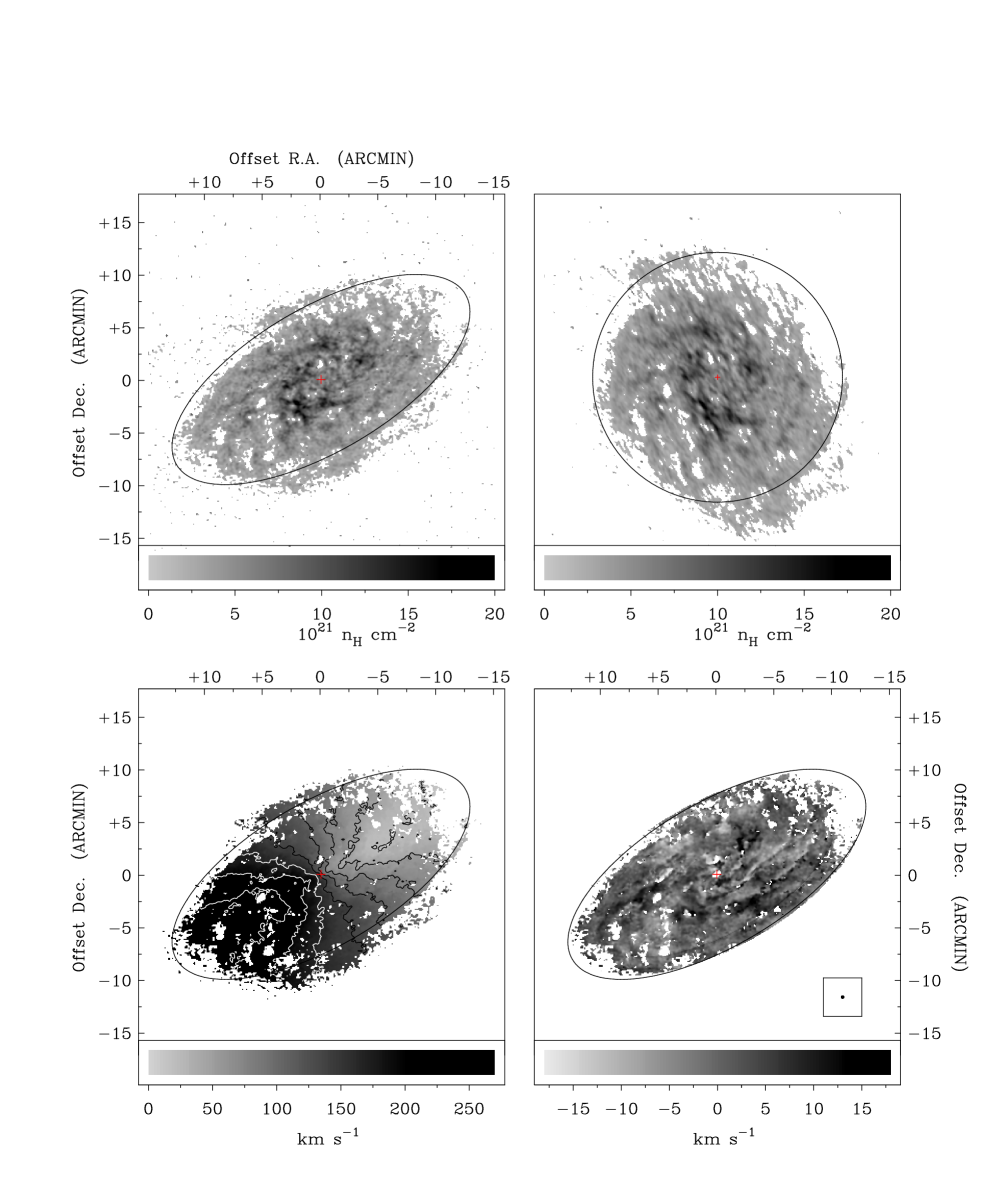
Figure 3: WSRT observations of NGC 2403. Top left: Map of the H i surface density. Some spiral-like structure is visible. The ellipse is the outermost ring fitted to the data in the tilted–ring decomposition. Top right: The deprojected H i image of NGC 2403 (deprojected with constant inclination). Bottom left: The velocity field. Systemic velocity is at 133.5 km s^-1. The contours range from 20 km s^-1 to 260 km s^-1 and are spaced 30 km s^-1 apart. Bottom right: The residual velocity field. Here we have subtracted the result of a tilted–ring fit from the original velocity field. Some structure can be seen. Note the small amplitude of the residuals (less than 10%) with respect to the original field. The beam size is indicated in the box in the lower right corner.

NGC 2403 is a nearby (3.25 Mpc Begeman 1987) Sc(s)III galaxy [Sandage & Tammann 1981]. It has been observed $4\times 12$ hours with the WSRT [Sicking 1997]. The data have been smoothed to a circular beam of 13 arcseconds. With this beam and a pixel size of $5\times 5.5$ arcseconds, the $\beta$-factor of equation (12) is $3.73$.

NGC 2403 is well suited for our analysis:

1. It has a large extent on the sky (Holmberg dimensions $29^{\prime}.0\times 15^{\prime}.0$)

2. It has a favourable inclination ($i\approx 62\degr$)

3. The data is of high signal/noise and has a small beam

4. The galaxy shows no obvious warp

Figure 3 shows the surface density map of the H i gas in the upper left corner. All data with a $\mbox{S/N}<3$ is clipped away, in order to have a reliable velocity field. The ellipse is the outermost ring ($R=858$ arcsec) fitted to the velocity and surface density fields. Outside this radius, the data has suffered too much from clipping to make a sensible harmonic decomposition possible. The centre of all the rings is indicated by a red cross and was kept fixed during the tilted–ring fit.

Next to this map we present the deprojected H i surface density map. We took an inclination of $62\degr$ to deproject the galaxy, the average value found by the tilted–ring fits. NGC 2403 seems to be a bit elongated in the direction of the (apparent) minor axis. Some traces of spiral arms can be seen.

At the bottom left the velocity field is shown. It is relatively regular apart from some small wiggles in the iso-velocity contours, probably caused by spiral arms. Next to the velocity map is the residual velocity field, created by subtracting the fitted circular velocity from the true velocity field. The residuals are not large ($<10$ km s^-1 in absolute magnitude) and appear to show some systematic, three-fold, structure. The beam shape is indicated in the lower right corner.

5.2 Results of the harmonic expansion

Figure 4: Harmonic expansion and ring parameters of NGC 2403 as a function of radius. Average values of the ring parameters are indicated by a dashed line. The points are separated by 26 arcsec ($2$ beams) and are therefore independent. The Holmberg radius is indicated by an arrow at the end of the box (at 870 arcsec). The amplitude of the $\hat{s}_{3}$ term is the largest with an amplitude $\approx 3$ km s^-1. This is about $2\%$ of the rotation velocity $\hat{c}_{1}$. At the bottom the average amplitude ($A_{i}=\sum_{j}(\hat{c}_{i}(j)^{2}+\hat{s}_{i}(j)^{2})^{1/2}/j$, $A_{1}=\sum_{j}\sqrt{\hat{s}_{1}^{2}(j)}/j$) of the harmonic terms is plotted.

The first step in our procedure is to expand the velocity field of NGC 2403 into individual concentric tilted–rings. The parameters $i$, $\Gamma$ and $v_{\rm sys}$ are measured locally for each ring, in order to be able to use the exact formalism of Appendix A3. We took the width of each ring to be 26 arcseconds, i.e., 2 beams. Therefore, the individual points in the plots of Figure 4 can be considered independent. Figure 4 presents the inclination, position angle and systemic velocity of each ring as a function of radius. The fluctuations in the inclination $i$ and position angle $\Gamma$ are most probably caused by an $m=2$ spiral arm in the density. In the case of $\varphi_{2}(R)\neq 0$, the measured inclination will in general not be equal to the true inclination, as mentioned before. This will cause the measured inclination to wiggle around its average value. We expect this average value to be very close to the true inclination. The fluctuations in the systemic velocity, $\hat{c}_{0}$, are of comparable magnitude as the $\hat{c}_{2},\hat{s}_{2}$ terms, as it should be according to Appendix 3.1 if these variations are caused by an $m=1$ term in the surface density. It should resemble $-\hat{c}_{2}$, but if $\hat{c}_{2}$ is also influenced by an $m=3$ term in the density, this need not exactly be the case. The weighted average values of the ring parameters are:

1. position angle: $124\aas@@fstack{\circ}2\pm 0\aas@@fstack{\circ}04$

2. inclination: $61\aas@@fstack{\circ}8\pm 0\aas@@fstack{\circ}18$

3. systemic velocity: $133.5\pm 0.09$ km s^-1

In Figure 4 we also present the result of the harmonic expansion of the tilted–rings. The arrow just beyond the last measured point denotes the Holmberg radius. This means that our H i observations are completely within the optical disk of NGC 2403.

After an initial rise, the rotation curve of NGC 2403 is relatively flat within errors. The $\hat{c}_{3}$ term has been fitted to zero by the tilted–ring fit, indicating that the inclination has been fitted correctly to the rings (but note again that in the case of an $m=2$ spiral arm, this inclination is not identical to the true inclination of the ring). There is some $\hat{c}_{4}$ at radii smaller than $400$ arcsec that may be caused by an $m=3$ component in the potential. This $m=3$ component may also influence the $\hat{c}_{2}$ and $\hat{s}_{2}$ harmonics. These $\hat{s}_{2}$ and $\hat{c}_{2}$ terms are relatively large and are probably caused by an $m=1$ component in the potential. The $\hat{s}_{3}$ term is the strongest harmonic found in NGC 2403. This term is negative at all radii. We can calculate $\epsilon_{\rm pot}\sin 2\varphi_{2}$ from $\hat{s}_{1}$ and $\hat{s}_{3}$ at each radius as (cf. eq. [9])

$$\epsilon_{\rm pot}\sin 2\varphi_{2}={(\hat{s}_{3}-\hat{s}_{1}){(1+2q^{2}+5q^{4})\over\hat{c}_{1}(1-q^{4})}}$$ (13)

Figure 5 shows $\epsilon_{\rm pot}\sin 2\varphi_{2}$ as a function of radius. It shows significant variations, but is negative at all radii. As we saw in the numerical examples of the previous paragraph, spiral arms would cause a radially alternating pattern of positive and negative values for the $\hat{s}_{3}$ kinematic term, whereas a global elongation would cause the $\hat{s}_{3}$ term to be constant and non-zero throughout the disk. A possible explanation for the behaviour of the measured $\hat{s}_{1}$,$\hat{s}_{3}$ is therefore that the average value of $\epsilon_{\rm pot}\sin 2\varphi_{2}$ is caused by a global elongation of the disk and that the wiggles superposed on it are due to spiral arms. The weighted average value of $\epsilon_{\rm pot}\sin 2\varphi_{2}$ is $-0.064\pm 0.003$. Since $\epsilon_{\rm pot}\sin 2\varphi_{2}$ has only physical meaning in the case of a more or less flat rotation curve, it should only be trusted outside about 200 arcsec. Harmonics higher than $m=5$ have small amplitudes.

Figure 5: The elongation measurement as calculated from the $\hat{s}_{1}$,$\hat{s}_{3}$ and inclination (eq. 13). It varies as a function of radius, but is negative throughout the galaxy. A possible explanation for this behaviour is that the average value of $\epsilon_{\rm pot}\sin 2\varphi_{2}$ is caused by some global elongation and the wiggling is caused by other effects like spiral arms. The average value is $-0.064\pm 0.003$

6 NGC 3198

6.1 Data description

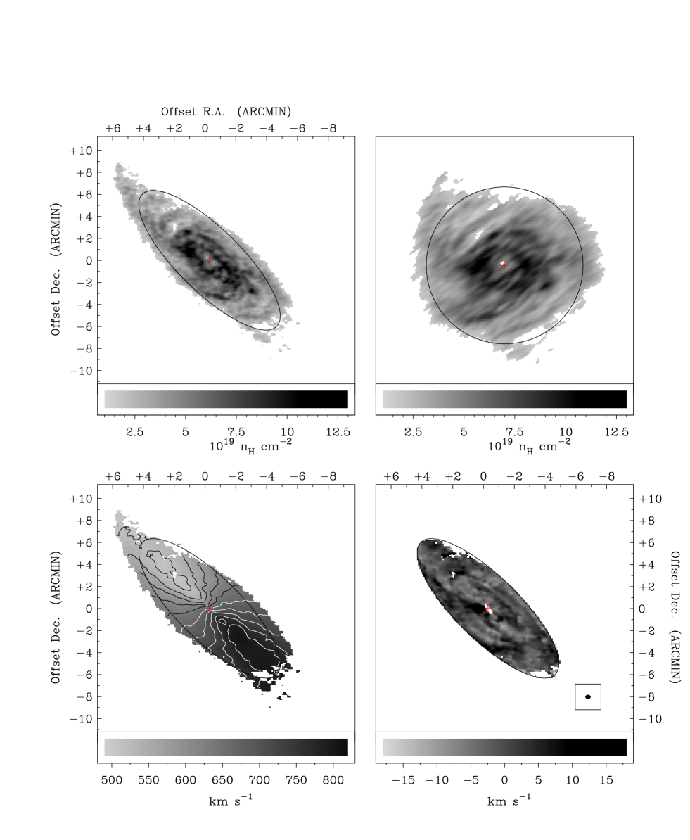
Figure 6: WSRT observations of NGC 3198. Top left: Map of the H i surface density. Some spiral-like structure is visible outside an H i ring-like structure. The ellipse is the outermost ring that has been fitted to the data. Top right: The deprojected H i image of NGC 3198 (deprojected with constant inclination). The structure and H i ring is better visible here. Bottom left: The velocity field. The systemic velocity is at 659.6 km s^-1. The contours range from 520 km s^-1 to 790 km s^-1 and are spaced 30 km s^-1 apart. Bottom right: The residual velocity field. Here we have subtracted the result of a tilted–ring fit from the original velocity field. There is some four-fold structure visible. The beam size is indicated in the box in the lower right corner.

The second relatively nearby (9.4 Mpc, Begeman 1987) spiral galaxy we will examine is the Sc(rs)I-II [Sandage & Tammann 1981] galaxy NGC 3198. This galaxy was observed $4\times 12$ hours with the WSRT [Sicking 1997]. The observations were subsequently reprojected to a circular beam with FWHM of $18$ arcsec. The $\beta$ factor, equation (12), for NGC 3198 is $4.6$.

NGC 3198 also meets our criteria:

1. It has large dimensions on the sky (Holmberg dimensions $11^{\prime}.9\times 4^{\prime}.9$)

2. The inclination is $i\approx 71\degr$

3. The data is of high S/N and has a small beam

4. NGC 3198 has no warp of significance

In Figure 6 we present the data for this galaxy. The data is of somewhat better quality than the data for NGC 2403, since the disk of NGC 3198 is completely filled, although the beam is larger. The surface density field shows a ring-like structure of a few arcminutes, with 3 spiral-like structures extending from it. The ellipses and the circle again indicate the outermost data used for the harmonic analysis ($450$ arcsec in this case). The cross indicates the position of the centre of the rings. The velocity field of NGC 3198 is quite regular and the amplitudes of the residual field are not very large, typically less than 10 km s^-1 in both the positive and negative direction. Even though these residuals are small, they do show some systematic structure. It is worth noting that the residuals are strongest near the centre of NGC 3198.

6.2 Results of the harmonic expansion

Figure 7: Harmonic decomposition and ring parameters of NGC 3198 as a function of radius. Average values are indicated as a dashed line. The points are seperated by $1.7$ beams and are therefore independent. The Holmberg radius is indicated by an arrow. The total amplitude, bottom graph, decreases as a function of harmonic number. The systemic velocity $\hat{c}_{0}$ varies a few km s^-1 over the galaxy, comparable in amplitude with the largest harmonics. The position angle $\Gamma$ varies a few degrees as a function of radius. The inclination $i$ is constant within measurement errors.

We fitted a set of concentric rings to the velocity field of NGC 3198. We present the results for the ring parameters in Figure 7. The systemic velocity, $c_{0}$, varies with an amplitude of a few km s^-1, about the same amplitude variation as the strongest terms in the harmonic decomposition. The inclination of the rings, $i$, is constant within errors. The position angle $\Gamma$ varies a few degrees. The weighted values of the ring parameters found are:

1. position angle: $216\aas@@fstack{\circ}0\pm 0\aas@@fstack{\circ}05$

2. inclination: $70\aas@@fstack{\circ}5\pm 0\aas@@fstack{\circ}20$

3. systemic velocity: $659.6\pm 0.15$ km s^-1

Figure 7 also presents the result of the subsequent harmonic fit. After an initial rise, the rotation curve is flat within errors up to the last measured point at 450 arcsec. This is not the outermost limit of the observed H i distribution (see Figure 6) but since the disk shows big gaps at radii larger than 450 arcsec, the harmonic expansion would become too unreliable. The arrows denote the Holmberg radius, so our measurements go out to about 1.3 Holmberg radii.

As predicted by the theory, the $\hat{c}_{3}$ term has been fitted to zero by the tilted–ring fit. Together with the fact that the inclination is constant as a function of radius, this tells us that NGC 3198 does not contain strong $m=2$ spiral arms, although a global elongation of the disk is still possible. The $\hat{c}_{2},\hat{s}_{2}$ terms are quite strong in the inner part of NGC 3198. The centre has been fixed at such a value as to minimize the $\hat{c}_{2},\hat{s}_{2}$ terms. As a consequence the $\hat{s}_{2},\hat{c}_{2}$ terms are relatively small in the outer part of NGC 3198. If the centre is left as a free parameter in the tilted-ring fit, it drifts by a few hundred parsec in order to make the $\hat{c}_{2},\hat{s}_{2}$ terms zero. In other words, NGC 3198 is somewhat lop-sided.

In the surface density map we saw that there appear to be three spiral-like structures in the H i . This would cause some non-zero $m=2$ and $m=4$ terms in the kinematic expansion of the velocity field. Indeed, we see that there is some power in the $\hat{c}_{4},\hat{s}_{4}$ terms that may be caused by an $m=3$ component in the H i field.

Finally, there is a strong $\hat{s}_{3}$ term, together with a less strong $\hat{s}_{1}$ term. From these two terms we deduce $\epsilon_{\rm pot}\sin 2\varphi_{2}$ as a function of radius, as plotted in Figure 8. The low amplitude of $\epsilon_{\rm pot}\sin 2\varphi_{2}$ is striking: its weighted average is $-0.019\pm 0.003$. This low value may be caused by $\epsilon_{\rm pot}$ itself being small, or the viewing angle $\varphi_{2}$ being such as to make $\sin 2\varphi_{2}$ much smaller than unity. The variation in $\epsilon_{\rm pot}\sin 2\varphi_{2}$ can be due to the variation of $\epsilon_{\rm pot}$ with radius, or $\varphi_{2}(R)$ is not completely zero, or a combination of both.

Figure 8: Elongation $\epsilon_{\rm pot}\sin 2\varphi_{2}$, as measured from the $\hat{s}_{1}$, $\hat{s}_{3}$ terms and inclination. Its radial variation is not very large within errors, indicating that global ellipticity might be the cause of the non-zero measurement, and its average amplitude is low ($-0.019\pm 0.003$). The arrow indicates the Holmberg radius.

7 Summary and discussion

We have extended the FvGdZ formalism for measuring elongation of potentials to the case of a slightly non-axisymmetric filled gas disk, which may contain spiral-like perturbations. All the details of this derivation can be found in the Appendix. This analysis assumes a stationary perturbation in the frame rotating with the perturbation, and closed stable orbits. According to this analysis, a perturbation in the potential of harmonic number $m$ causes an $m-1$ and $m+1$ perturbation in the radial velocity field. The $m-1$ component will be dominant in amplitude if $\Omega_{0}>\Omega_{b}$, otherwise the $m+1$ component will be dominant. Applicability to non-linear phenomena like spiral arms is limited. But a small global elongation of the overall potential, as is the case with a triaxial dark matter halo, can be analysed with our method. In the case of a triaxial potential, we have $m=2$, small pattern speed and no radial dependence of the phase of the $m=2$ perturbation. If we assume a flat rotation curve, we can deduce $\epsilon_{\rm pot}\sin 2\varphi_{2}$. Here, $\epsilon_{\rm pot}$ is equal to the ellipticity of the potential and $\varphi_{2}$ is the angle between the minor axis of the elliptical orbit plus a phase term and the viewing angle. The term $\epsilon_{\rm pot}\cos 2\varphi_{2}$ cannot be determined. In order to measure this $\epsilon_{\rm pot}\sin 2\varphi_{2}$ and other perturbations of velocity fields, we need to expand the gas disk into individual rings. This was done by fitting a tilted–ring model to the velocity fields. A tilted-ring model tries to fit a circular model to the velocity field. Given the rings found by the tilted–ring fit, we made a harmonic expansion of the velocity field along each ring. In that way we obtain the harmonic terms $\hat{c}_{n},\hat{s}_{n}$ as a function of $R$, where we took $n\leq 9$ for our fits. Given $\hat{s}_{1}(R)$ and $\hat{s}_{3}(R)$, we can calculate $\epsilon_{\rm pot}\sin 2\varphi_{2}$ as a function of radius. Other perturbations of the velocity field, like spiral arms, do not affect the elongation measurement, unless they contain some $m=2$ or $m=4$ component in the potential. In that case, the global elongation and the other perturbing effect cannot be uniquely disentangled. We propose that the absolute mean value of $\epsilon_{\rm pot}\sin 2\varphi_{2}$ is an upper limit of the true elongation and the wiggling is caused by spiral arms. Since the method relies on the fact that the velocity in each point in the velocity field is uniquely determined, the method cannot be applied in those parts of galaxies where strong warping is evident.

Two spiral galaxies with regular H i velocity fields were analysed with this method: NGC 2403 and NGC 3198. Both galaxies show less power in the higher order ($m>5$) terms than in the lower order terms.

NGC 2403 clearly shows spiral-like behaviour. Its $\hat{s}_{3}$ term is large and negative at all radii and the amplitude changes as a function of radius. Two effects can contribute to this measurement: a global elongation of the disk causing a constant non-zero $\hat{s}_{3}$ and spiral arms, as are visible in the surface density map, that cause the wiggles. The radially averaged $|\langle\epsilon_{\rm pot}\sin 2\varphi_{2}\rangle|$ is $0.064\pm 0.003$.

NGC 3198 shows signs of spiral arms in the $m=4$ kinematic mode (in the H i surface density map a three-armed spiral-like structure can be seen). The relatively large $\hat{s}_{2},\hat{c}_{2}$ terms in the central parts may be caused by lop-sidedness of the galaxy and the $\hat{s}_{1},\hat{s}_{3}$ terms are most probably caused by global elongation. The deduced value for $|\langle\epsilon_{\rm pot}\sin 2\varphi_{2}\rangle|$ is $0.019\pm 0.003$.

We conclude that both galaxies may show signs of small global elongation ($<0.1$), although it is hard to separate the effects of spiral arms, global elongation and viewing angles. On the other hand, the sum of the effects of spiral arms and global elongation is small, which means that the two galaxies are close to axisymmetry. But in order to quantify this result, more galaxies need to be analyzed in this way. Work along these lines is in progress (Schoenmakers et al., in prep.).

Appendix A Harmonic analysis of the velocity field of a filled gas disk

A.1 Deprojection of the line-of-sight velocity

Let $R$ and $\theta$ be polar coordinates in the rest frame of the galaxy and consider a rotating, non-axisymmetric potential in that frame. It can be written as:

$$V(R,\theta,t)=V_{0}(R)+\sum_{m}V_{m}(R)\cos\{m[\theta-\Omega_{p,m}t-\phi_{m}(R)]\}.$$ (14)

The potential of a single perturbation in a frame that rotates with the potential perturbation:

$$V(R_{\rm orbit},\phi_{\rm orbit})=V_{0}(R_{\rm orbit})+V_{m}(R_{\rm orbit})\cos\{m[\phi_{\rm orbit}-\phi_{m}(R_{\rm orbit})]\},$$ (15)

where $V_{0}(R_{\rm orbit})$ is the unperturbed potential and $V_{m}(R_{\rm orbit})\cos\{m[\phi_{\rm orbit}-\phi_{m}(R_{\rm orbit})]\}$ is the perturbation. The subscript ”orbit” denotes that these coordinates describe the point on the closed loop orbit with guiding centre on $(R_{0},\phi_{0})$.

The derivation given in this Appendix is also valid for a summation of perturbations and the final result is a linear addition of the results for the individual perturbations. There is some coupling between different terms that occurs when calculating $v_{\phi}$, equation (A.1), but this coupling occurs in second order equations only and can be ignored in first order calculations.

Following the treatment of Binney & Tremaine (1987, p. 146), we find that the solution for closed loop orbits is:

$$R_{\rm orbit} =R_{0}+\delta R= R_{0}\left(1-\textstyle{\frac{a_{1m}}{2}}\cos\eta-a_{2m}\sin\eta\right),$$

$$\phi_{\rm orbit} =\phi_{0}+\delta\phi= \phi_{0}+\textstyle{\frac{(a_{1m}+a_{3m})}{2m}}\sin\eta-a_{4m}\cos\eta,$$ (16)

$R_{0}$ and $\phi_{0}$ denote those solutions to the unperturbed problem that represent a circular orbit ($R=R_{0},\phi=\phi_{0}=(\Omega_{0}-\Omega_{p,m})t$). $\Omega_{0}$ is the circular frequency: $\Omega_{0}\equiv\sqrt{V_{0}^{\prime}/R}$ and $\Omega_{p,m}$ is the pattern speed of the particular perturbation. $\delta R$ and $\delta\phi$ denote the perturbations on the circular orbit. The extra terms with respect to the analysis of Binney & Tremaine arise from the additional phase term $\phi_{m}(R_{\rm orbit})$ in the potential. Furthermore:

$$\eta=\eta(m,R_{\rm orbit}) = m[(\Omega_{0}-\Omega_{p,m})t-\phi_{m}(R_{\rm orbit})]\equiv m[\phi_{0}-\phi_{m}(R_{\rm orbit})],$$

$$a_{1m} = \frac{2}{\Delta_{0}}\left[{2\Omega_{0}V_{m}\over R_{0}(\Omega_{0}-\Omega_{p,m})}+V_{m}^{\prime}\right],$$

$$a_{2m} = {mV_{m}\phi_{m}^{\prime}(R_{\rm orbit})\over\Delta_{0}},$$ (17)

$$a_{3m} = \frac{2}{\Delta_{0}}\left\{{V_{m}[(2+m^{2})\Omega_{0}^{2}+2(1-m^{2})\Omega_{0}\Omega_{p,m}+m^{2}\Omega_{p,m}^{2}-\kappa_{0}^{2}]\over R_{0}(\Omega_{0}-\Omega_{p,m})^{2}}+{(\Omega_{0}+\Omega_{p,m})\over(\Omega_{0}-\Omega_{p,m})}V_{m}^{\prime}\right\},$$

$$a_{4m} = {2\Omega_{0}V_{m}\phi_{m}^{\prime}(R_{\rm orbit})\over\Delta_{0}(\Omega_{0}-\Omega_{p,m})},$$

where differentiation with respect to $R$ is denoted as ^′, $\Delta_{0}=R_{0}\left[\kappa_{0}^{2}-m^{2}(\Omega_{0}-\Omega_{p,m})^{2}\right],$ and $\kappa_{0}^{2}\equiv 3\Omega_{0}^{2}+V_{0}^{\prime\prime}$, the usual epicycle frequency. These equations break down near resonances.

The velocities in a frame at rest with respect to the observer are:

$$v_{R} = mv_{c}(1-\omega_{m})\left(\textstyle{\frac{1}{2}}a_{1m}\sin\eta-a_{2m}\cos\eta\right),$$

$$v_{\phi} = v_{c}\left\{1+\textstyle{\frac{1}{2}}[(1-\omega_{m})a_{3m}-\omega_{m}a_{1m}]\cos\eta-[m(1-\omega_{m})a_{4m}-a_{2m}]\sin\eta\right\},$$ (18)

where $\omega_{m}\equiv{\Omega_{p,m}\over\Omega_{0}}$ and $v_{c}(R_{0})=R_{0}\Omega_{0}$, the circular velocity.

So far we only looked at what happens to a single orbit. A complete velocity field consists of many orbits and the circular velocity may be a function of radius. Suppose we are observing the point $(R,\phi)$ in the velocity field. What is the orbit that goes through this point, in other words, what is the $(R_{0},\phi_{0})$ that corresponds to $(R,\phi)$?

Let us write equation (A.1) as

$$R_{\rm orbit}(t,R_{0},\phi_{0})=R_{0}\left[1+r(R_{0},\phi_{0})\right], \phi_{\rm orbit}(t,R_{0},\phi_{0})=\phi_{0}+p(R_{0},\phi_{0}).$$ (19)

Then to first order the coordinates for the guiding centre of the orbit going through $(R,\phi)$ are

$$R_{0}=\frac{R}{1+r(R,\phi)}, \phi_{0}=\phi-p(R,\phi).$$ (20)

Then

$$v_{c}(R_{0}) = v_{c}(R)(1-r{d\ln v_{c}(R)\over d\ln R}),$$

$$\omega(R_{0}) = \omega(R)(1-r{d\ln\omega(R)\over d\ln R}).$$ (21)

Inserting these equations in equation A.1 and retaining only first order terms, we find

$$v_{R} = mv_{c}(R)[1-\omega_{m}(R)]\left(\textstyle{{1\over 2}}a_{1m}\sin\eta-a_{2m}\cos\eta\right),$$

$$v_{\phi} = v_{c}(R)\left\{1+\textstyle{{1\over 2}}[(1-\omega)a_{3m}+(\alpha-\omega_{m})a_{1m}]\cos\eta-[m(1-\omega_{m})a_{4m}-(1-\alpha)a_{2m}]\sin\eta\right\},$$ (22)

where $\alpha=\frac{d\ln v_{c}(R)}{d\ln R}$. The definition of $\alpha$ is such that the relation between the epicyclic frequency $\kappa_{0}$ and the circular frequency $\Omega_{0}$ can be written as $\kappa_{0}^{2}=2(1+\alpha)\Omega_{0}^{2}$.

We now project the velocity field on the sky. The line-of-sight velocity field is

$$v_{\rm los}(R)=[v_{R}\cos(\theta-\theta_{\rm obs})-v_{\phi}\sin(\theta-\theta_{\rm obs})]\sin i=[v_{R}\cos(\phi-\phi_{\rm obs})-v_{\phi}\sin(\phi-\phi_{\rm obs})]\sin i,$$ (23)

where $\phi_{\rm obs}$ is the angle between the line $\phi=0$ and the observer. The angle $i$ is the inclination of the plane of the disk with respect to the observer. Introduce the variable $\psi=\theta-\theta_{\rm obs}+{\pi\over 2}=\phi-\phi_{\rm obs}+{\pi\over 2}$. This coordinate is zero along the line of nodes. Then:

$$v_{\rm los}(R)=[v_{R}\sin\psi+v_{\phi}\cos\psi]\sin i.$$

Now replace $\phi\rightarrow\psi+\phi_{\rm obs}-{\pi\over 2}$ in the expressions for $v_{R}$ and $v_{\phi}$ and expand the line-of-sight velocity in multiple angles of $\psi$. Furthermore, define $v_{*}=v_{c}(R)\sin i$ and assume to first order $\phi_{0}\approx\phi$. After the expansion we find :

$$v_{\rm los}\!\! = \!\!c_{1}\cos\psi+s_{m-1}\sin(m\!-\!1)\psi+c_{m-1}\cos(m\!-\!1)\psi+s_{m+1}\sin(m\!+\!1)\psi+c_{m+1}\cos(m\!+\!1)\psi,$$ (24)

with

$$\!\!\!\!\!c_{1}\!\!\!\! = \!\!\!\!v_{*}$$

$$s_{m-1}\!\!\!\! = \!\!\!\!v_{*}(-\textstyle{\frac{1}{4}}\{[m\!-\!(m\!+\!1)\omega_{m}+\alpha]a_{1m}+(1\!-\!\omega_{m})a_{3m}\}\sin m\varphi_{m}\textstyle{+\frac{1}{2}}\left\{m(1\!-\!\omega_{m})a_{4m}+[m(1\!-\!\omega_{m})\!-\!1+\alpha]a_{2m}\right\}\cos m\varphi_{m}),$$

$$c_{m-1}\!\!\!\! = \!\!\!\!v_{*}(\textstyle{\frac{1}{4}}\{[m\!-\!(m\!+\!1)\omega_{m}+\alpha]a_{1m}+(1\!-\!\omega_{m})a_{3m}\}\cos m\varphi_{m}\textstyle{+\frac{1}{2}}\left\{m(1\!-\!\omega_{m})a_{4m}+[m(1\!-\!\omega_{m})\!-\!1+\alpha]a_{2m}\right\}\sin m\varphi_{m}),$$

$$s_{m+1}\!\!\!\! = \!\!\!\!v_{*}(\textstyle{\frac{1}{4}}\{[m\!-\!(m\!-\!1)\omega_{m}-\alpha]a_{1m}\!-\!(1\!-\!\omega_{m})a_{3m}\}\sin m\varphi_{m}\textstyle{+\frac{1}{2}}\left\{m(1\!-\!\omega_{m})a_{4m}-[m(1\!-\!\omega_{m})\!+\!1-\alpha]a_{2m}\right\}\cos m\varphi_{m}),$$ (25)

$$c_{m+1}\!\!\!\! = \!\!\!\!v_{*}(-\textstyle{\frac{1}{4}}\{[m\!-\!(m\!-\!1)\omega_{m}-\alpha]a_{1m}\!-\!(1\!-\!\omega_{m})a_{3m}\}\cos m\varphi_{m}\textstyle{+\frac{1}{2}}\left\{m(1\!-\!\omega_{m})a_{4m}-[m(1\!-\!\omega_{m})\!+\!1-\alpha]a_{2m}\right\}\sin m\varphi_{m}).$$

where $v_{*}=v_{c}\sin i$ and $\varphi_{m}=\phi_{\rm obs}-{\pi}/{2}-\phi_{m}(R)$.

A.2 Deprojection with incorrect viewing angles and incorrect centre

Now we investigate how the expansion of the line-of-sight velocity $v_{\rm los}=\sum_{i}c_{i}(R)\cos i\psi+s_{i}(R)\sin i\psi$ changes if an incorrect inclination $\hat{i}$, position angle $\hat{\Gamma}$ or centre $(\hat{x},\hat{y})$ is chosen. We will derive a general equation for the line-of-sight velocity which is also valid if a combination of these incorrect choices occur, since to first order we can simply add the contributions of the individual incorrect parameters.

Let us start with an incorrect inclination $\hat{i}=i+\delta i$, where $\delta i$ is the deviation from the correct value of the inclination $i$ and is assumed to be small. Then $\hat{q}=\cos(i+\delta i)=q+\delta q$. Using the equations for a projected circular orbit $x^{\prime\prime}=\hat{R}\cos\hat{\psi},y^{\prime\prime}=\hat{q}\hat{R}\sin\hat{\psi}$ and $\cos\psi=x^{\prime\prime}/R=x^{\prime\prime}/\sqrt{x^{\prime\prime 2}+y^{\prime\prime 2}/q^{2}}$ we find that the relation between $\cos\psi$ and $\cos\hat{\psi}$ is

$$\cos\psi=(1-\frac{\delta q}{4q})\cos\hat{\psi}+\frac{\delta q}{4q}\cos{3\hat{\psi}}.$$ (26)

Or, more general

$$\cos a\psi=\cos a\hat{\psi}+\frac{a\delta q}{4q}\left(\cos(a+2)\hat{\psi}-\cos(a-2)\hat{\psi}\right)+{\cal O}(\delta q^{2}).$$ (27)

and

$$R=\hat{R}[1+\frac{\delta q}{2q}(1-\cos 2\hat{\psi})]$$ (28)

Note that the amplitudes of the sine and cosine terms in equation (24) are first order, except the $\cos\psi$ term whose amplitude is $1$, and the corrections in equation (27) are first order too. Therefore, only the deprojection of the $\cos\psi$ term will give rise to first order contributions to the line-of-sight velocity.

Now define $\hat{\Gamma}=\Gamma+\delta\Gamma$, where $\Gamma$ is the correct position angle and $\delta\Gamma$ the deviation from it. In the same way as for the inclination we find

$$\cos\psi=\cos\hat{\psi}-{\delta\Gamma\over 4}\left[(3q+\frac{1}{q})\sin\hat{\psi}+(\frac{1}{q}-q)\sin 3\hat{\psi}\right].$$ (29)

More general

$$\cos a\psi=\cos a\hat{\psi}+\frac{a\delta\Gamma}{2q}\left\{\frac{(q^{2}-1)}{2}\left[\sin(a-2)\hat{\psi}+\sin(a+2)\hat{\psi}\right]-(1+q^{2})\sin a\hat{\psi}\right\}+{\cal O}(\delta\Gamma^{2}).$$ (30)

and

$$R=\hat{R}[1+\textstyle{\frac{1}{2}}(\textstyle{\frac{1}{q}}-q)\sin 2\hat{\psi}\delta\Gamma]$$ (31)

Again, only the deprojection of the $\cos\psi$ term will give rise to first order effects.

Finally let us consider an incorrect choice of the kinematic centre. Suppose the centre of the coordinate system is shifted from $(0,0)$ to $(x^{\prime},y^{\prime})$. Let us write this shift as $(\delta x,\delta y)$ where the $x$-axis coincides with the major axis of the projected orbit. Then

$$\cos\psi=\cos\hat{\psi}+{\delta x\over 2R}(1-\cos 2\hat{\psi})-{\delta y\over 2qR}\sin 2\hat{\psi}.$$ (32)

In general:

$$\cos a\psi=\cos a\hat{\psi}+{a\delta x\over{2R}}[\cos(a-1)\hat{\psi}-\cos(a+1)\hat{\psi}]+{a\delta y\over 2qR}\left[\sin(a-1)\hat{\psi}-\sin(a+1)\hat{\psi}\right]+{\cal O}(\delta x^{2},\delta y^{2}).$$ (33)

and

$$R=\hat{R}[1+{\delta x\over\hat{R}}\cos\hat{\psi}+{\delta y\over q\hat{R}}\sin\hat{\psi}]$$ (34)

Here too only the deprojection of the $\cos\psi$ term is important.

Define $dR=R-\hat{R}=\hat{R}[\textstyle{\frac{\delta q}{2q}}(1-\cos 2\hat{\psi})+\textstyle{\frac{1}{2}}(\textstyle{\frac{1}{q}}-q)\delta\Gamma\sin 2\hat{\psi}+{\delta x\over\hat{R}}\cos\hat{\psi}+{\delta y\over q\hat{R}}\sin\hat{\psi}]$ and substitute the relations between $\psi$ and $\hat{\psi}$ and $R$ and $\hat{R}$ into the expansion of $v_{\rm los}$. To first order $c_{i}(R)=c_{i}(\hat{R}+dR)=c_{i}(\hat{R})+dR(dc_{i}(\hat{R})/dR)$. Since ${dc_{i}/dR}$ is of the same order as $c_{i}$ and $dR$ is also small (order $\delta q$, $\delta\Gamma$, $\delta x,\delta y$), the only relevant term is $dc_{1}/dR$, the shape of the rotation curve (so this contribution is zero in the case of a flat rotation curve). Noting that $\hat{R}dc_{1}(\hat{R})/dR=v_{*}(\hat{R})\alpha$ we can expand the line-of-sight velocity in the case of incorrect viewing angles and centre as:

$$v_{\rm los} = v_{*}(\hat{R})\left\{(1+\alpha){\delta x\over 2R}-(1-\alpha){\delta q\over 4q}\cos\hat{\psi}-{\delta\Gamma\over 4}\left[(3q+{1\over q})-\alpha({1\over q}-q)\right]\sin\hat{\psi}-(1-\alpha){\delta x\over 2R}\cos 2\hat{\psi}\right.$$ (35)

$$\left.-(1-\alpha){\delta y\over 2qR}\sin 2\hat{\psi}+(1-\alpha){\delta q\over 4q}\cos 3\hat{\psi}-(1-\alpha){\delta\Gamma\over 4}({1\over q}-q)\sin 3\hat{\psi}\right\}+\sum_{i\geq 0}c_{i}(\hat{R})\cos i\hat{\psi}+s_{i}(\hat{R})\sin i\hat{\psi}.$$

If this is expanded into new harmonics, $v_{\rm los}=\sum_{i}\hat{c}_{i}(\hat{R})\cos i\hat{\psi}+\hat{s}_{i}(\hat{R})\sin i\hat{\psi}$, then $\hat{s}_{i}=s_{i},\hat{c}_{i}=c_{i}$, except for $i\leq 3$.

A.3 Deprojection under the assumption of a circular velocity field

Now we will calculate the errors in $\Gamma,i$ and centre if the general velocity field is deprojected under the assumption of a circular velocity field $v_{\rm los}=v_{*}\cos\hat{\psi}$. As a result, the $\chi^{2}$ deviation from the best fitting circular field is

$$\chi^{2}(\delta q,\delta\Gamma,\delta x,\delta y)\simeq\sum_{i\geq 0}(\hat{c}_{i}^{2}+\hat{s}_{i}^{2})-\hat{c}_{1}^{2},$$ (36)

where $\hat{s}_{i}$ and $\hat{c}_{i}$ are expressed in terms of the $\delta q$, $\delta\Gamma$, $\delta x$ and $\delta y$ in equation (35). The best fitting values of $\delta\Gamma$ and $\delta q$ are given by

$$\delta q=-\frac{4qc_{3}}{(c_{1}+c_{3})(1-\alpha)}, \delta\Gamma=4q{\left[(3q^{2}+1)-\alpha(1-q^{2})\right]s_{1}+(1-q^{2})(1-\alpha)s_{3}\over{\left\{[3q^{2}+1-(1-q^{2})\alpha]^{2}+(1-\alpha)^{2}(1-q^{2})^{2}]\right\}(c_{1}+c_{3})}}.$$ (37)

Equation (36) is minimized with respect to $\delta x$ and $\delta y$ when

$$\delta x=2Rc_{2}/(1-\alpha), \delta y=2qRs_{2}/(1-\alpha).$$ (38)

The resulting expressions for $\hat{c}_{i},\hat{s}_{i}$ under a circular fit are:

$$\hat{c}_{0}=c_{0}+{1+\alpha\over 1-\alpha}c_{2},$$

$$\hat{c}_{2}=0,$$ ^s_2 = 0,

$$\hat{c}_{1}=c_{1}[1\!-\!{\delta q\over 4q}(1\!-\!\alpha)]=c_{1}+c_{3},$$ ^s_1 = s_1 - c_1[(3q+1/q)-(1/q-q)α]δΓ/4, (39)

$$\hat{c}_{3}=c_{3}+(1-\alpha){\delta q\over 4q}c_{1}=0,$$ ^s_3 = s_3 - c_1(1/q - q)(1-α) δΓ/4.

A.3.1 Effect of $m=1$ distortion

For an $m=1$ distortion equation (A.1) gives the correct coefficients if the correct centre is chosen:

$$c_{0} = v_{*}{\textstyle{1\over 4}}\left[(1-2\omega_{1}+\alpha)a_{11}+(1-\omega_{1})a_{31}\right]\cos\varphi_{1}+{\textstyle{1\over 2}}[(1-\omega_{1})a_{41}+(\alpha-\omega_{1})a_{21}]\sin\varphi_{1},$$

$$c_{2} = -v_{*}{\textstyle{1\over 4}}\left[(1-\alpha)a_{11}-(1-\omega_{1})a_{31}\right]\cos\varphi_{1}+{\textstyle{1\over 2}}[(1-\omega_{1})a_{41}-(2-\omega_{1}-\alpha)a_{21}]\sin\varphi_{1},$$ (40)

$$s_{2} = v_{*}{\textstyle{1\over 4}}\left[(1-\alpha)a_{11}-(1-\omega_{1})a_{31}\right]\sin\varphi_{1}+{\textstyle{1\over 2}}[(1-\omega_{1})a_{41}-(2-\omega_{1}-\alpha)a_{21}]\cos\varphi_{1}.$$

If the velocity field itself is used to derive the centre, these equations reduce according to equation (A.3) to:

$$\hat{c}_{0} = v_{*}{\textstyle{1\over 2(\alpha-1)}}\left\{[(1-\alpha)\omega_{1}a_{11}-(1-\omega_{1})a_{31}]\cos\varphi_{1}-2[(1-\omega_{1})a_{41}+(\alpha\omega_{1}-1)a_{21}]\sin\varphi_{1}\right\},$$

$$\hat{c}_{2} = 0,$$ (41)

$$\hat{s}_{2} = 0.$$

These terms are not affected by an error in $q$ and $\Gamma$.

A.3.2 Effect of $m=2$ distortion

With $m=2$, equation (A.1) gives the coefficients if a correct inclination and position angle are chosen:

$$c_{1} = v_{*}\left\{1-\textstyle{\frac{1}{4}}\left[(2-3\omega_{2}+\alpha)a_{12}+(1-\omega_{2})a_{32}\right]\cos 2\varphi_{2}+\textstyle{\frac{1}{2}}\left[2(1-\omega_{2})a_{42}+(1-2\omega_{2}+\alpha)a_{22}\right]\sin 2\varphi_{2}\right\},$$

$$s_{1} = v_{*}\left\{-\textstyle{\frac{1}{4}}\left[(2-3\omega_{2}+\alpha)a_{12}+(1-\omega_{2})a_{32}\right]\sin 2\varphi_{2}+\textstyle{\frac{1}{2}}\left[2(1-\omega_{2})a_{42}+(1-2\omega_{2}+\alpha)a_{22}\right]\cos 2\varphi_{2}\right\},$$

$$c_{3} = v_{*}\left\{-\textstyle{\frac{1}{4}}\left[(2-\omega_{2}-\alpha)a_{12}-(1-\omega_{2})a_{32}\right]\cos 2\varphi_{2}+\textstyle{\frac{1}{2}}\left[2(1-\omega_{2})a_{42}-(3-2\omega_{2}-\alpha)a_{22}\right]\sin 2\varphi_{2}\right\},$$ (42)

$$s_{3} = v_{*}\left\{-\textstyle{\frac{1}{4}}\left[(-2+\omega_{2}+\alpha)a_{12}+(1-\omega_{2})a_{32}\right]\sin 2\varphi_{2}+\textstyle{\frac{1}{2}}\left[2(1-\omega_{2})a_{42}-(3-2\omega_{2}-\alpha)a_{22}\right]\cos 2\varphi_{2}\right\}.$$

When the velocity field itself is used to derive the position angle and inclination, we find using equation (A.3):

$$\hat{c}_{1} = v_{*}\left\{1+\textstyle{\frac{1}{2}}\left[(\alpha-\omega_{2})a_{12}+(1-\omega_{2})a_{32}\right]\cos 2\varphi_{2}+[2(1-\omega_{2})a_{42}+(\alpha-1)a_{22}]\sin 2\varphi_{2}\right\},$$

$$\hat{s}_{1} = v_{*}\left\{-\textstyle{\frac{1}{4}}\left[(2-3\omega_{2}+\alpha)a_{12}+(1-\omega_{2})a_{32}\right]\sin 2\varphi_{2}+\textstyle{\frac{1}{2}}[2(1-\omega_{2})a_{42}+(1-2\omega_{2}+\alpha)a_{22}]\cos 2\varphi_{2}-\right.$$

$$\left.-{[3q^{2}\!\!+\!\!1\!\!+\!\!\alpha(q^{2}\!\!-\!\!1)](\left\{2(1\!\!-\!\!\alpha)(\omega_{2}\!\!-\!\!\alpha)+2[2\!\!-\!\!\alpha^{2}\!\!-\!\!4\omega_{2}\!\!+\!\!\alpha(2\!\!+\!\!\omega_{2})]q^{2}\right\}a_{12}\!\!-\!\a_{32})\over{4[1+2q^{2}+5q^{4}+\alpha^{2}(1-q^{2})^{2}+2\alpha(q^{4}-1)]}}\sin 2\varphi_{2}-\right.$$

$$\left.-{[3q^{2}\!\!+\!\!1\!\!+\!\!\alpha(q^{2}\!\!-\!\!1)]\left\{4[1\!\!+\!\!q^{2}\!\!-\!\!\alpha(1\!\!-\!\!q^{2})](1\!\!-\!\!\omega_{2})a_{42}-2[1\!\!-\!\!(3\!\!-\!\!4\omega_{2})q^{2}\!\!-\!\!\alpha(1\!\!+\!\!q^{2})]a_{22}\right\}\over{4[1+2q^{2}+5q^{4}+\alpha^{2}(1-q^{2})^{2}+2\alpha(q^{4}-1)]}}\cos 2\varphi_{2}\right\},$$

$$\hat{c}_{3} = 0,$$ (43)

$$\hat{s}_{3} = v_{*}\left\{-\textstyle{\frac{1}{4}}\left[(\omega_{2}+\alpha-2)a_{12}+(1-\omega_{2})a_{32}\right]\sin 2\varphi_{2}+\textstyle{\frac{1}{2}}[2(1-\omega_{2})a_{42}-(3-2\omega_{2}-\alpha)a_{22}]\cos 2\varphi_{2}+\right.$$

$$\left.+{(1\!\!-\!\!\alpha)(1\!\!-\!\!q^{2})(\left\{2(1\!\!-\!\!\alpha)(\omega_{2}\!\!-\!\!\alpha)+2[2\!\!-\!\!\alpha^{2}\!\!-\!\!4\omega_{2}\!\!+\!\!\alpha(2\!\!+\!\!\omega_{2})]q^{2}\right\}a_{12}\!\!-\!\a_{32})\over 4{[1+2q^{2}+5q^{4}+\alpha^{2}(1-q^{2})^{2}+2\alpha(q^{4}-1)]}}\sin 2\varphi_{2}+\right.$$

$$\left.+{(1\!\!-\!\!\alpha)(1\!\!-\!\!q^{2})\left\{4[1\!\!+\!\!q^{2}\!\!-\!\!\alpha(1\!\!-\!\!q^{2})](1\!\!-\!\!\omega_{2})a_{42}\!\!-\!\!2[1\!\!-\!\!(3\!\!-\!\!4\omega_{2})q^{2}\!\!-\!\!\alpha(1\!\!+\!\!q^{2})]a_{22}\right\}\over{4[1+2q^{2}+5q^{4}+\alpha^{2}(1-q^{2})^{2}+2\alpha(q^{4}-1)]}}\cos 2\varphi_{2}\right\}.$$

These equations are independent of a small error in the position of the centre. For a triaxial non-rotating halo model, in which the potential is scale free, we have $\omega_{2}=0$, $\alpha=0$ (flat rotation curve), the phase of the perturbation is constant with radius $\varphi_{2}(R)\sim\mbox{const}$ (therefore $a_{42}=a_{22}=0$), $a_{32}=2a_{12}=2\epsilon_{\rm pot}$ (FvGdZ) and these equations simplify to the equations (2.2).

A.3.3 Solid body rotation

Let us finally consider the effect of solid body rotation, $\alpha=1$. Equations (37) and (38) show that in this case it is impossible to measure the inclination. Indeed, in solid body rotation, all iso-velocity contours are parallel and each inclination fits equally well. The position angle on the other hand can be determined, $\delta\Gamma={s_{1}\over q}$. Centre and systemic velocity cannot be determined uniquely. Therefore, assumptions for all these parameters have to be made in order to get a rotation velocity. It is not possible to interpret harmonic terms under these conditions in the way we did in this Appendix.

References

- [Barnes 1994] Barnes, J., 1994, in The Formation and Evolution of Galaxies, eds C. Munoz-Tunón & F. Sanchez (Cambridge Univ. Press), p. 401
- [Begeman 1987] Begeman K., PhD-thesis, University of Groningen, 1987
- [Binney 1978] Binney J., 1978, MNRAS, 183, 779
- [Binney & Tremaine 1987] Binney J., Tremaine S., Galactic Dynamics , 1987, Princeton University Press
- [Binney & de Vaucouleurs 1981] Binney J., de Vaucouleurs G., 1981, MNRAS, 194, 679
- [Canzian 1993] Canzian B., 1993, Ap.J., 414, 487
- [Cole & Lacey 1996] Cole S., Lacey C., MNRAS, 281, 716
- [Dubinski 1994] Dubinski J., 1994, Ap.J., 431, 617
- [Dubinski & Carlberg 1991] Dubinski J., Carlberg R.G., 1991, Ap.J., 378, 496
- [Fasano et al 1992] Fasano G., Amico P., Bertola F., Vio R., Zeilinger W.W., 1992, MNRAS, 262, 109
- [Franx & de Zeeuw 1992] Franx M.,de Zeeuw P.T., 1992, Ap.J., 392, L47
- [Franx, van Gorkom, de Zeeuw 1994] Franx M., van Gorkom J.M., de Zeeuw P.T., 1994, Ap.J., 436, 642 (FvGdZ)
- [Gradshteyn & Ryzhik 1965] Gradshteyn I.S., Ryzhik I.M., 1965, Table of Integrals, Series and Products, New York: Academic
- [Holmberg 1958] Holmberg E., 1958, Medd. Lund Obs. Ser. II, 136
- [van der Hulst et al. 1992] van der Hulst J.M., Terlouw J.P., Begeman K., Zwitser W., Roelfsema P.R., 1992, “The Groningen Image Processing System, GIPSY”, in: Astronomical Data Analysis Software and Systems I, (eds. D. M. Worall, C. Biemesderfer and J. Barnes), ASP Conf. series no. 25, p. 131.
- [Katz & Gunn 1991] Katz N., Gunn J.E., 1991, Ap.J., 377, 365
- [Kuijken & Tremaine 1994] Kuijken K., Tremaine S., 1994, Ap.J., 178, 421
- [Lambas et al 1992] Lambas D.G., Maddox S.J., Loveday J., 1992, MNRAS, 258, 404
- [van der Marel 1991] van der Marel R., 1991, MNRAS, 248, 515
- [Navarro, Frenk & White 1996] Navarro J.F., Frenk C.S., White S.D.M., 1996, Ap.J., 462, 563
- [Olling 1995a] Olling R.P., 1995a, AJ, 110, 591
- [Olling 1995b] Olling R.P., 1995b, BAAS, 187, 48.05
- [Rix & Zaritsky 1995] Rix H-W., Zaritsky D., 1995, Ap.J., 447, 82
- [Sackett et al. 1994] Sackett P.D., Rix H-W.,Jarvis B.J., Freeman K.C., 1994, Ap.J., 436, 629
- [Sackett & Sparke 1990] Sackett P.D., Sparke L.S., 1990, Ap.J., 361, 408
- [Sandage & Tammann 1981] Sandage A., Tammann G.A., 1981, Revised Shapley-Ames Catalogue of Bright Galaxies (Carnegie Inst. of Washington Pub. No. 635)
- [Sicking 1997] Sicking F.J., PhD-thesis, University of Groningen, 1997
- [Teuben 1991] Teuben P., 1991, in Warped Disks and Inclined Rings around Galaxies, (eds. S. Casertano, P.Sackett, F. Briggs), Cambridge Univ. Press.
- [Tohline, Simonson & Caldwell, 1982] Tohline J.E., Simonson G.F., Caldwell N., 1982, Ap.J., 252, 92
- [Warren et al. 1992] Warren M.S., Quinn P.J., Salmon J.K, Zurek W.H., 1992, Ap.J., 399, 405
- [Whitmore, McElroy & Schweizer 1987] Whitmore B.C., McElroy D., Schweizer F., 1987, Ap.J., 314, 439
- [Lin & Shu 19??]