TTF: A Flexible Approach to Narrowband Imaging

Abstract

The Taurus Tunable Filter (TTF) is a tunable narrowband interference filter covering wavelengths from 6300Å to the sensitivity drop-off of conventional CCDs ($\sim 9600$ Å), although a blue ‘arm’ (3700$-$6500Å) is to be added by the end of 1997. The TTF offers monochromatic imaging at the cassegrain foci of both the Anglo-Australian and William Herschel Telescopes, with an adjustable passband of between 6 and 60 Å. In addition, frequency switching with the TTF can be synchronized to movement of charge (charge shuffling) on the CCD which has important applications to many astrophysical problems. Here we review the different modes of TTF and suggest their use for follow-up narrowband imaging to the AAO/UKST Galactic Plane H$\alpha$ Survey.

¹ Anglo-Australian Observatory, P.O. Box 296, Epping, NSW 2121
jbh@aaossz.aao.gov.au
² Mount Stromlo & Siding Spring Observatories,
Private Bag, Weston Creek P.O., ACT 2611
dhj@mso.anu.edu.au

Keywords: instrumentation: detectors — methods: observational
   — techniques: interferometric

1 INTRODUCTION

The Taurus Tunable Filter (TTF), manufactured by Queensgate Instruments Pty. Ltd., has the appearance of a conventional Fabry-Perot etalon in that it comprises two highly polished glass plates. Unlike conventional Queensgate etalons, however, the TTF incorporates very large piezo-electric stacks (which determine the plate separation) and high performance coatings over half the optical wavelength range. Moreover, the plate separation can be tuned to spacings as small as 2$\mu$m (measured at the coating surfaces). The TTF is used in the collimated beam of the TAURUS-2 focal reducer available at both the 3.9 m Anglo-Australian (AAT) and 4.2 m William Herschel (WHT) telescopes. Field coverage is 10 arcmin at f/8 or 5 arcmin at f/15.

For the first time, TTF provides the capability to synchronize frequency switching with the movement of charge on a CCD, or charge shuffling. This has important benefits for many astrophysical experiments, not least for averaging out temporal variations due to the atmosphere or measurement apparatus. This instrument is an important step in changing the way that intermediate to narrowband imaging is performed at observatories.

The TTF has largely removed the need for buying arbitrary narrow and intermediate interference filters, as one can tune the bandpass and the centroid of the bandpass by selecting the plate spacing. The spacing of the plates is controlled to extremely high accuracy with a capacitance bridge (Jones & Richards 1968). This approach to tunable imaging has existed since the instrument of Atherton & Reay (1981), although TTF is the first of its kind in terms of both wavelength and bandpass accessibility. Since tunable filters have a periodic transmission profile, the instrument requires a limited number of blocking filters. At low resolution ($R=300$), conventional broadband $R$ and $I$ filters suffice. At high resolution ($R=1000$), eight intermediate band filters are used to sub-divide $R$ and $I$.

The highly polished plates are coated for optimal performance over 6300-9600 Å. The coating reflectivity (96 %) determines the shape and degree of order separation of the instrumental profile. This is fully specified by the coating finesse, $N$, which has a quadratic dependence on the coating reflectivity. The TTF was coated to a finesse specification of $N=40$ which means that the separation between periodic profiles is forty times the width of the instrumental profile. At such high values, the profile is Lorentzian to a good approximation. For a given wavelength, changes in plate spacing, $L$, correspond to different orders of interference, $m$. This in turn, dictates the resolving power $R=Nm$ according to the finesse.

In the following sections we summarise the different observing modes of TTF. Discussion is also made of phase effects in the field and their influence. The flexibility of TTF will see it well-suited to narrowband follow-up from the AAO/UKST Galactic Plane H$\alpha$ Survey, in lines such as H$\alpha$, [NII]$\lambda$6583, [SII]$\lambda$6717 and [SII]$\lambda$6731.

We maintain a WWW site (http://msowww.anu.edu.au/$\sim$dhj/ttf.html) describing all aspects of TTF and its operation. In addition to general use, the instrument is available for AAT service time (http://www.aao.gov.au/local/www/jmc/service/service.html) if observations are shorter than 3 hours.

2 CCD CHARGE SHUFFLING

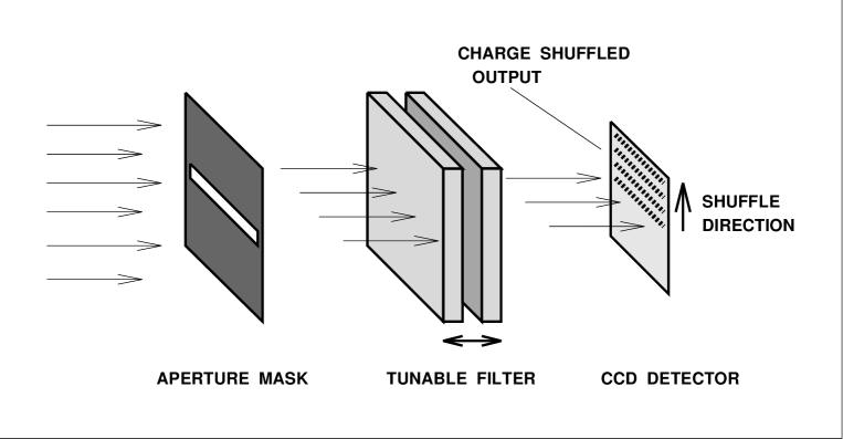
Figure 1: Simplified view of how the CCD chip is illuminated and shuffled. The mask aperture size controls the amount of the CCD exposed and therefore the number of different images fit on to an individual frame. Charge can be shuffled in both up and and down the chip.

Central to almost all modes of TTF use is charge shuffling. Charge shuffling is movement of charge along the CCD between multiple exposures of the same frame, before the image is read out (Clemens & Leach 1987, Cuillandre et al. 1994). An aperture mask ensures only a section of the CCD frame is exposed at a time. For each exposure, the tunable filter is systematically moved to different gap spacings in a process called frequency-switching. This way, a region of sky can be captured at several different wavelengths on the one image (Fig. 1). Alternatively, the TTF can be kept at fixed frequency and charge shuffling performed to produce time-series exposures. Each of these modes is described in the following section.

The TTF plates can be switched anywhere over the physical range 2 to 12 $\mu$m at rates in excess of 100 Hz, although in most applications, these rates rarely exceed 0.1 Hz. If a shutter is used, this limits the switching rate to about 1 Hz. Charge on a large format CCD can be moved over the full area at rates approaching 10 Hz: it is only when the charge is read out through the amplifiers that this rate is greatly slowed down. The TTF exploits the ability of certain large format CCDs to move charge up and down many times before significant signal degradation occurs (Yang et al. 1989). In this way, it is possible to form discrete images taken at different frequencies where each area of the detector may have been shuffled into view many times to average out temporal effects.

The field of view available in shuffle mode depends on the number of frequencies being observed. When we move the charge upwards, say, information in pixels at the top of the field is rolled off the top and lost. For example, two frequencies requires that we divide the CCD into three vertical partitions where information in one of the outer partitions is lost in the shuffle process. In the limit of $n$ frequencies, where $n$ is large, only half the available detector area is used to store information. The new MIT-LL 4096 x 2048 (rows $\times$ columns) format CCDs will increase the detector area available for shuffling by a factor of 4 compared to the present Tek 1024$\times$1024 CCD. This is because the instrument field of view projects to an aperture 1024 pixels in diameter and shuffling is only possible in the vertical direction.

One application of charge shuffling that does not sacrifice detector area is time-series imaging (Section 3.3, below). This is because the imaging region is relatively small and able to be read out as the time-series progresses.

3 OBSERVING MODES OF TTF

There are several technical problems driving the development of tunable filters for narrowband imaging over standard fixed interference filters. First, it is difficult and very expensive for manufacturers to produce high performance narrow passbands, particularly at resolving powers approaching 1000. This problem is largely circumvented by use of TTF in conjunction with a 5-cavity, intermediate bandpass blocking filter. Secondly, the TTF instrumental function has identical form at all wavelengths and all bandpasses. A comparison of two discrete bands at different wavelengths is moderated only by the blocking filter transmission at those wavelengths (which is normally flat in any case), and the ratio of the gap spacings. Thirdly, the same optical path is used at all frequencies. Furthermore, the ability to shuffle charge allows one to average out all temporal variations: atmospheric transparency, the contribution from atmospheric lines, seeing, detector and electronic instabilities.

We now describe some of the advantages to be had from the TTF shuffle capability in imaging emission-line sources.

3.1 Tuning to a Specific Wavelength and Bandpass

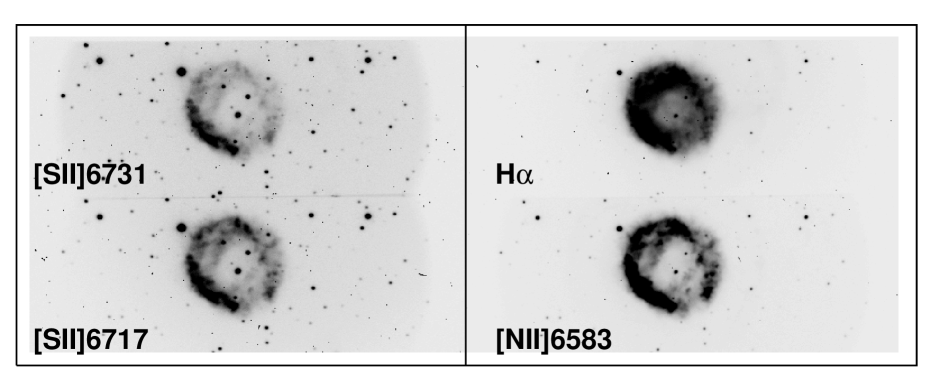
(a) (b)
(c)

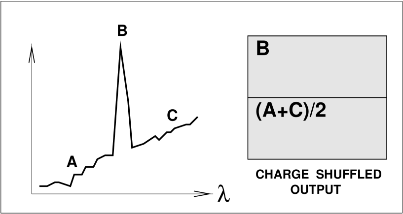
Figure 2: ($a$) Charge shuffled image of the planetary nebula NGC 2438 in [SII]$\lambda$6371 (top) and [SII]$\lambda$6717 (bottom). The TTF was frequency-switched 18 times during the 12 min exposure and the charge shuffled back and forth in concert. A 10 Å bandpass was used. ($b$) Charge shuffle time-series imaging of V2116 Oph, an x-ray pulsar in orbit around a red giant. V2116 Oph is to the right, reference stars are at the centre and left. TTF was tuned to a 7 Å bandpass centred on the [OI]$\lambda$8446 line, which is suspected to vary with the pulsar period of 120 s. Each exposure was 12 s. ($c$) Charge shuffling either side of an emission-line to average out the effect of a steeply sloping continuum. Equal time is spent collecting continuum from both sides of the emission line.

This allows us to obtain images of obscure spectral lines at arbitrary redshifts (see e.g. Jones & Bland-Hawthorn 1997a). We can also optimize the bandpass to accomodate the line dispersion and to suppress the sky background. The off-band frequency can be chosen to avoid night-sky lines and can be much wider so that only a fraction of the time is spent on the off-band image. Fig. 2($a$) shows a charge-shuffled image of the planetary nebula NGC 2438 in [SII] lines at 6731 and 6717 Å. During this 12 min exposure, TTF was switched between the two frequencies 18 times while the charge was shuffled back and forth accordingly. In this way, temporal variations in atmospheric transmission are equally shared between each passband over the entire exposure time.

3.2 Shuffling Between On and Off-band Frequencies

With the new MIT-LL chips, we are able to image the full 10 arcmin field for two discrete frequencies. We can also choose a narrow bandpass for the on-band line and a much broader bandpass (factor of 4-5) for the off-band image so that we incur only a 20 % overhead for the off-band image. As with specific tuning (Section 3.1, above), multiple frequencies can be imaged in a single frame, the number of which is entirely arbitrary.

3.3 Time-Series Imaging

For time-varying sources, we can step the charge in one direction while only switching between a line and a reference frequency. For example, a compact variable source imaged through a narrow aperture in the focal plane forms a narrow image at the detector. We can switch between the line and a reference frequency many times forming a set of narrow interleaved images at the detector. The reference frequency is a measure of the atmospheric stability during the time series. Alternatively, if nearby reference stars are available for photometric calibration, then charge shuffling can be done at a single fixed frequency as demonstrated in Fig 2($b$). For example, some x-ray binaries produce strong emission lines that vary on 0.1 Hz timescales.

An important difference between time-series and multi-frequency shuffles is that the former does not sacrifice any detector area. This is possible only when charge shuffling occurs in the same direction as normal CCD read out. For example, with a slit only 4 pixels wide, we can obtain 500 images in the emission line, interleaved with a further 500 images at a reference frequency.

3.4 Adaptive Frequency Switching with Charge Shuffling

When imaging spectral lines that fall between OH bandheads or on steeply rising continua, a powerful feature is the ability to shuffle between on and off bands but where the off band is alternated between two or more frequencies either side of the on-band frequency. As illustrated in Fig. 2, this can be used to average out either rapid variations in blocking filters or the underlying spectral continuum.

3.5 Shuffling Charge in One Direction with a Narrow Focal Plane Slit

This allows us to produce a long-slit spectrum of an extended source. While this is vastly less efficient than using a long-slit spectrograph, this is a fundamental requirement for establishing the parallelism of reflecting mirrors at few micron spacings (Jones & Bland-Hawthorn 1997b). Conventional methods are an order of magnitude slower.

4 PHASE EFFECTS

The primary goal of a tunable filter is to provide a monochromatic field over as large a detector area as possible. With the present TTF, however, the field of view is not strictly monochromatic. The effect is most acute at high orders of interference. Fig. 3($a$) shows how wavelength gradients (or phase effects) are evident from a ring pattern of atmospheric OH emission lines across the TTF field.

Wavelengths are longest at the centre and get bluer the further one moves off-axis. For instruments such as TTF, the wavelength as a function of off-axis angle $\theta$ is

$$\lambda(\theta)=\lambda_{\rm centre}\cdot\Bigl{(}1-\frac{\theta^{2}}{2}\Bigr{)}.$$ (1)

Here $\lambda_{\rm centre}$ is the on-axis wavelength, equal to $2L/m$ (for an air gap), where $L$ is the physical plate spacing and $m$ is the order of interference.

It follows from Eqn. (1) that the change in wavelength $\lambda_{\phi}$ across an angle $\theta$ from the centre is given by

$$\lambda_{\phi}(\theta)=\lambda_{\rm centre}\cdot\frac{\theta^{2}}{2}.$$ (2)

Since $\theta\leq 0.14$ for the current Tektronix CCD, then $\lambda_{\phi}/\lambda_{\rm centre}$ is always $\lower 2.15277pt\hbox{$\,\buildrel<\over{\sim}\,$}10^{-2}$. It also follows that $\lambda_{\phi}/\lambda_{\rm centre}$ remains fixed over a given radius, irrespective of order $m$. Bland & Tully (1989) derive similar equations in the context of a higher order conventional etalon.

We define our monochromatic field by the size of the Jacquinot spot, the central region of the ring pattern. By definition, the Jacquinot spot is the region over which the wavelength changes by no more than $\sqrt{2}$ of the etalon bandpass, $\delta\lambda$. For wavelength, $\lambda$, the bandpass relates directly to the order $m$ such that

$$\delta\lambda=\lambda/Nm=\lambda/(40\times m).$$ (3)

Here, $N$ is the effective finesse of the etalon, which in the case of TTF is approximately 40. Combining Eqns. (1) and (3) we find that the angle subtended by the Jacquinot spot is

$${\theta_{\rm Jac}}^{2}=2\sqrt{2}/Nm{\rm\,\,}=1/(14.1\times m).$$ (4)

For a particular etalon, the size of the Jacquinot spot depends on order $m$ alone. Eqn. (4) shows how the spot covers increasingly larger areas on the detector as the filter is used at lower orders order of interference. The absolute wavelength change across the detector remains the same, independently of order. However, its effect relative to the bandpass diminishes as $m$ decreases. Fig. 3($b$) demonstrates how the effects of atmospheric emission can be removed during reduction.

The TTF is the most straightforward application of tunable filter technology. Other, more sophisticated techniques such as acousto-optic filters exist, (see Bland-Hawthorn & Cecil 1996 for a review), although all are currently considerably more expensive. In future TTF-type instruments, phase effects will be eliminated from the outset by bowed plates. One advantage of such a design is that the TTF will no longer have to be tilted to deflect ghost reflections. Furthermore, interference coatings are notorious for bowing plates and this can be factored into the plate curvature specification. Other possible improvements are additional cavities to square up the instrument profile. All of these modifications are currently being explored.

5 SUMMARY

We have discussed details of the Taurus Tunable Filter (TTF) instrument and its use. When used in conjunction with a CCD charge shuffling technique, TTF is well-suited for multi-narrowband imaging of emission-line sources. As such, it is ideal for follow-up imaging to the AAO/UKST Galactic Plane H$\alpha$ Survey, for sources that are $\sim 10$ arcmin or smaller. The analysis of tunable filter data is more straightforward than traditional Fabry-Perot imaging as all regions of the field are close to a common wavelength.

The present TTF instrument exhibits some phase effects at high resolving powers. We have demonstrated that these effects are tolerable for most applications ($\lambda_{\phi}/\lambda_{\rm centre}\lower 2.15277pt\hbox{$\,\buildrel<\over{\sim}\,$}10^{-2}$) and the side-effects correctable through software. The commissioning of TTF has marked the start of an exciting period of new imaging instruments for optical astronomy.

References

Atherton, P. D. and Reay, N. K. 1981 MNRAS 197, 507

Bland, J. and Tully, R. B. 1989 AJ 98(2), 723

Bland-Hawthorn, J. and Cecil, G. N. 1996 in Atomic, Molecular and Optical Physics: Atoms and Molecules, vol. 29B, ch. 18, eds. Dunning, F. B. and Hulet, R. G., Academic Press, (astro-ph/9704142)

Clemens, D. P. and Leach, R. W. 1987 Opt. Eng. 26, 9

Cuillandre, J. C., Fort, B., Picat, J. P., Soucail, G., Altieri, B., Beigbeder, F., Dupin, J. P., Pourthie, T. and Ratier, G. 1994, Astron. Astrophys. 281, 603

Jones, H. and Bland-Hawthorn, J. 1997a PASA, 14, 8

Jones, D. H. and Bland-Hawthorn, J. 1997b Appl. Opt., in prep.

Jones, R. V. and Richards, J. C. S. 1973 J. Phys. E. 6, 589

Yang, F. H., Blouke, M. M., Heidtmann, D. L., Corrie, B., Riley, L. D.  and Marsh, H. H. 1989 in Optical Sensors and Electronic Photography (Proc. SPIE), eds. Blouke, M. M. and Pophal, D., SPIE – International Society for Optical Engineering, 213

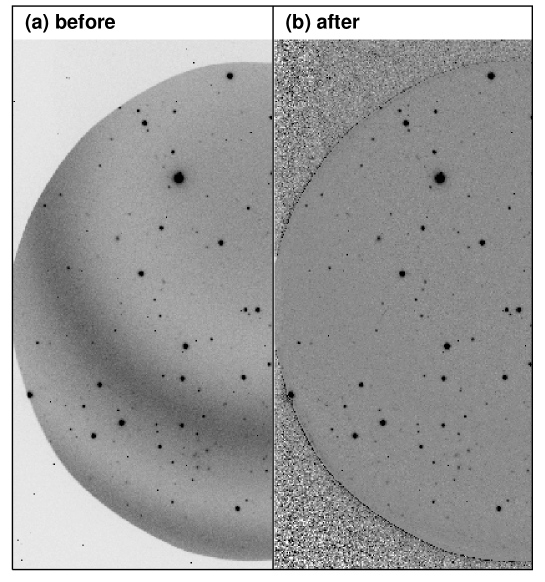
Figure 3: Images showing the removal of the atmospheric OH emission lines from a raw TTF image before ($a$) and after ($b$) cleaning. Only half the full TTF field is shown in each case.