RESCEU-26/97

OCHA-PP-100

UTAP-265/97

ACCURACY OF NONLINEAR APPROXIMATIONS IN SPHEROIDAL COLLAPSE
— Why are Zel’dovich-type approximations so good? —

Ayako Yoshisato¹, Takahiko Matsubara^2,3 and Masahiro Morikawa¹

¹Department of Physics, Ochanomizu University, 2-2-1, Otsuka, Bunkyo-ku 112, Japan.

²Department of Physics, The University of Tokyo, Tokyo 113, Japan.

²Research Center for the Early Universe, Faculty of Science, The University of Tokyo, Tokyo 113, Japan.

ABSTRACT

Among various analytic approximations for the growth of density fluctuations in the expanding Universe, Zel’dovich approximation and its extensions in Lagrangian scheme are known to be accurate even in mildly non-linear regime. The aim of this paper is to investigate the reason why these Zel’dovich-type approximations work accurately beyond the linear regime from the following two points of view: (1) Dimensionality of the system and (2) the Lagrangian scheme on which the Zel’dovich approximation is grounded. In order to examine the dimensionality, we introduce a model with spheroidal mass distribution. In order to examine the Lagrangian scheme, we introduce the Padé approximation in Eulerian scheme. We clarify which of these aspects supports the unusual accuracy of the Zel’dovich-type approximations. We also give an implication for more accurate approximation method beyond the Zel’dovich-type approximations.

Subject headings: cosmology: theory — galaxies: clustering — gravitation — large-scale structure of universe

1 Introduction

As an analytic approximation for the growth of density fluctuations in the expanding Universe, Zel’dovich approximation (ZA hereafter) is known to be unusually accurate even in mildly non-linear regime for unknown reason (Zel’dovich 1970; 1973). Recently the extensions of this ZA (Post- and Post-post- Zel’dovich Approximations, PZA and PPZA hereafter) have been developed (e.g., Bernardeau 1994; Buchert 1994; Bouchet et al. 1995). These Zel’dovich-type approximations are confirmed to be far better than any other analytic approximations in Munshi, Sahni & Starobinsky (1994), Sahni & Shandarin (1995) and Sahni & Coles (1996) using a spherical-collapse model. However so far, there has been no clear explanation why these Zel’dovich-type approximations are so accurate beyond their range of applicability. In this paper, we would like to address this issue from limited aspects and with limited models.

In the Zel’dovich-type approximations, we work on the Lagrangian coordinate scheme in which the location of a mass element ${\bf x}$ of the fluid is expressed by the initial location ${\bf q}$ and the time dependent displacement vector $\Psi$ as

$${\mbox{\boldmath$x$}}({\mbox{\boldmath$q$}},t)={\mbox{\boldmath$q$}}+{\mbox{\boldmath$\Psi$}}({\mbox{\boldmath$q$}},t).$$ (1.1)

Then the density contrast $\delta[{\mbox{\boldmath$x$}}({\mbox{\boldmath$q$}},t),t]=\det[\partial x_{i}/\partial q_{j}]^{-1}-1$ is determined by solving the equation of motion

$$\frac{d^{2}{\mbox{\boldmath$\Psi$}}}{dt^{2}}+2H\frac{d{\mbox{\boldmath$\Psi$}}}{dt}=-\nabla_{x}\Phi({\mbox{\boldmath$x$}},t),$$ (1.2)

$$\nabla_{x}^{\,2}\Phi=\frac{3}{2}H^{2}\Omega\delta({\mbox{\boldmath$x$}},t),$$ (1.3)

where $\nabla_{x}$ is the spatial derivative with respect to Eulerian coordinates $x$. This nonlinear equation for $\Psi$ can be solved by the method of iteration considering $\partial{\mit\Psi}_{i}/\partial q_{j}$ to be a small parameter. The first iteration corresponds to the ZA. With further iterations, PZA and PPZA are considered to improve the accuracy.

There seem to be at least two possible grounds for the Zel’dovich-type approximations:

• In the plain parallel mass distribution, equations (1.2) and (1.3), with $\delta=1/(1+{\mit\Psi}^{\prime})-1$, reduce to

  $$\frac{d^{2}{\mit\Psi}^{\prime}}{dt^{2}}+2H\frac{d{\mit\Psi}^{\prime}}{dt}=\frac{3}{2}H^{2}\Omega{\mit\Psi}^{\prime},$$ (1.4)

  where ${\mit\Psi}^{\prime}=\partial{\mit\Psi}/\partial q$. This differential equation (1.4) is exactly the same as that for the linear density contrast $\delta_{\rm L}$, thus ${\mit\Psi}^{\prime}\propto\delta_{\rm L}$.Therefore, in this case, ZA becomes exact at least before shell crossings occur. This one-dimensional-exact property is considered to support the validity of this approximation also in three-dimensional systems.

• ZA is unique in the sense that it is based on the Lagrange coordinate scheme while all the other nonlinear approximations are based on the Eulerian coordinate scheme. This fact may make the ZA extraordinary excellent.

In this paper, we would like to clarify the reason why Zel’dovich-type approximations are so good from the above limited points of view.

In order to elucidate the aspect (1), we introduce a model of spheroidal collapse. In the previous analytical work (Munshi et al. 1994; Sahni & Shandarin 1995; Bouchet et al. 1995) only spherical symmetric models, which are analytically solvable, have been used to examine the validity of the Zel’dovich-type approximations. By changing the axes ratio in our spheroidal model, we can freely control the effective dimensionality of the system. For example, a prolate collapse is effectively dimension two and an oblate collapse is effectively dimension one. Therefore, if the one-dimensional-exact property in the first aspect (1) in the above gives the very reason for the Zel’dovich-type approximations, their accuracy would be the best in oblate collapse and may be better in prolate collapse than in spherical collapse.

In order to explore the aspect (2), we introduce the Padé approximation in Eulerian coordinate scheme. This is not a simple polynomial expansion with a small parameter but a rational polynomial expansion. In this paper, we compare this sophisticated approximation in the Eulerian scheme with Zel’dovich-type approximations in Lagrangian scheme. If the aspect (2) gives the very reasoning for the Zel’dovich-type approximations, their accuracy is far better than this Padé approximation.

In the course of our study, we need to establish the hierarchy of accuracy in various nonlinear approximations. Therefore we examine the other known nonlinear approximations in Eulerian scheme such as (a) linear perturbation and higher order perturbation approximations, (b) frozen-flow approximation, and (c) linear-potential approximation, as well as Zel’dovich-type approximations and the Padé approximation.

The organization of this paper is as follows: In section two, we summarize various nonlinear approximations in gravitational instability theory. They are applied to the spheroidal perturbation model in section three. The first aspect is examined in this section. In section four, we introduce the Padé approximation in Eulerian scheme. The second aspect is examined in this section. In section five, we clarify which aspects are supported from our analysis. In the last section six, we conclude our analysis and briefly mention the possibility of the approximation scheme beyond the Zel’dovich-type approximations.

2 Nonlinear Approximations in Gravitational Instability Theory

2.1 Equations of motion and linear perturbation scheme

In the gravitational instability theory, the non-relativistic matter with zero pressure in an Einstein-de Sitter universe is described by the following set of equations (see e.g., Peebles 1980),

$$\dot{\delta}+\nabla\cdot[(1+\delta){\mbox{\boldmath$v$}}]=0,$$ (2.1)

$$\dot{{\mbox{\boldmath$v$}}}+2H{\mbox{\boldmath$v$}}+({\mbox{\boldmath$v$}}\cdot\nabla){\mbox{\boldmath$v$}}+\nabla\Phi=\bf 0,$$ (2.2)

$$\nabla^{2}\Phi=\frac{3}{2}H^{2}\delta,$$ (2.3)

where $x$, ${\mbox{\boldmath$v$}}({\mbox{\boldmath$x$}},t)$, $\Phi({\mbox{\boldmath$x$}},t)$ are respectively position, peculiar velocity, peculiar potential in comoving coordinate, which correspond to $a{\mbox{\boldmath$x$}}$, $a{\mbox{\boldmath$v$}}$, $a^{2}\Phi$ in physical coordinate. An over dot denotes the time derivative and $\nabla\equiv\partial/\partial{\mbox{\boldmath$x$}}$ denotes the spatial derivative with respect to comoving coordinates. The scale factor $a$ varies as $a\propto t^{2/3}$ and the Hubble parameter is $H=\dot{a}/a=2/(3t)$. Although we consider Einstein-de Sitter universe throughout this paper, it is straightforward to generalize our analysis to $\Omega\neq 1,\Lambda\neq 0$ universes.

For these non-linear equations, we show various approximations in the following. In the linear regime ($\delta\ll 1$), we can safely neglect the nonlinear terms and obtain relatively simple solution (see, e.g., Peebles 1980). Neglecting decaying mode, the solution is

$$\delta_{\rm L}({\mbox{\boldmath$x$}},t)=\frac{a(t)}{a_{\rm in}}\delta_{\rm in}({\mbox{\boldmath$x$}}),$$ (2.4)

$$\Phi_{\rm L}({\mbox{\boldmath$x$}},t)=\frac{3}{2}H^{2}\triangle^{-1}\delta_{\rm L},$$ (2.5)

$${\mbox{\boldmath$v$}}_{\rm L}({\mbox{\boldmath$x$}},t)=-\frac{2}{3H}\nabla\Phi_{\rm L},$$ (2.6)

where $\triangle^{-1}$ is the inverse Laplacian:

$$\triangle^{-1}F({\mbox{\boldmath$x$}})\equiv-\frac{1}{4\pi}\int d^{3}x^{\prime}\frac{F({\mbox{\boldmath$x$}}^{\prime})}{|{\mbox{\boldmath$x$}}^{\prime}-{\mbox{\boldmath$x$}}|}.$$ (2.7)

These quantities simply evolve as $\delta_{\rm L}\propto a,\quad\Phi_{\rm L}\propto a^{-2},\quad{\mbox{\boldmath$v$}}_{\rm L}\propto a^{-1/2}$.

For the later convenience, we introduce the peculiar potential $\phi=a^{2}\Phi$. In Einstein-de Sitter universe, the linear peculiar potential is constant, $\phi_{\rm L}({\mbox{\boldmath$x$}},t)={\rm const.}\equiv\phi({\mbox{\boldmath$x$}})$.

2.2 Higher order perturbation methods in Eulerian scheme

In higher order perturbation methods, nonlinear correction terms are added to the linear solution; $\delta=\delta_{\rm L}+\delta^{(2)}+\delta^{(3)}+\cdots$, $\Phi=\Phi_{\rm L}+\Phi^{(2)}+\Phi^{(3)}+\cdots$, ${\mbox{\boldmath$v$}}={\mbox{\boldmath$v$}}_{\rm L}+{\mbox{\boldmath$v$}}^{(2)}+{\mbox{\boldmath$v$}}^{(3)}+\cdots$, where $\delta^{(n)}$ $\Phi^{(n)}$ ${\mbox{\boldmath$v$}}^{(n)}$ is assumed to be of order $(\delta_{\rm L})^{n}$. This expansion enables us to solve the nonlinear equations (2.1)-(2.3) order by order. The second-order expression of the perturbation is relatively simple (e.g., see Peebles 1980; Fry 1984):

$$\delta=\delta_{\rm L}+\frac{5}{7}\delta_{\rm L}^{\,2}+\delta_{{\rm L},i}\varphi_{{\rm L},i}+\frac{2}{7}\varphi_{{\rm L},ij}\varphi_{{\rm L},ij}$$ (2.8)

where $\varphi=\triangle^{-1}\delta_{\rm L}$. However, the expression of higher order is complicated. For the detailed expression of the third and fourth-order solution in Fourier space, see Goroff et al. (1986). The explicit expression for the higher order is not necessary for our analysis, so is not quoted here.

2.3 Frozen flow and linear potential approximations

Matarrese et al. (1992) introduced the frozen flow approximation (FF, hereafter). In this approximation, the velocity field ${\mbox{\boldmath$v$}}({\mbox{\boldmath$x$}},t)$ is kept fixed to the value of linear perturbation scheme:

$${\mbox{\boldmath$v$}}_{\rm FF}\left({\mbox{\boldmath$x$}},t\right)=-\frac{2}{3a^{2}H}\nabla_{x}\phi_{\rm L}({\mbox{\boldmath$x$}}),$$ (2.9)

A particle in FF moves simply along the line determined by the fixed linear velocity fields (2.9), i.e., the position of each particle, ${\mbox{\boldmath$x$}}(t)$, is described by the differential equation,

$$\frac{d{\mbox{\boldmath$x$}}}{dt}=-\frac{2}{3a^{2}H}\nabla_{x}\phi_{\rm L}({\mbox{\boldmath$x$}}(t)).$$ (2.10)

where $d/dt$ is the Lagrangian time derivative. It is convenient to rewrite the equations as follows:

$$\frac{d{\mbox{\boldmath$x$}}}{da}=-\frac{2}{3a^{3}H^{2}}\nabla_{x}\phi_{\rm L}({\mbox{\boldmath$x$}}).$$ (2.11)

On the other hand, Brainerd, Scherrer & Villumsen (1993) and Bagla & Padmanabham (1994) introduced linear potential approximation (LP, hereafter) which is based on the assumption that the gravitational potential evolves according to the linear perturbation scheme. As a result, particles effectively move along the lines of force of the initial potential $\phi_{\rm in}$. Thus the position of each particle ${\mbox{\boldmath$x$}}(t)$ is described by the differential equation,

$$\frac{d^{2}{\mbox{\boldmath$x$}}}{dt^{2}}+2H\frac{d{\mbox{\boldmath$x$}}}{dt}=-\frac{1}{a^{2}}\nabla_{x}\phi_{\rm L}({\mbox{\boldmath$x$}}).$$ (2.12)

This equation is also rewritten as follows:

$$\frac{d^{2}{\mbox{\boldmath$x$}}}{da^{2}}+\frac{3}{2a}\frac{d{\mbox{\boldmath$x$}}}{da}+\frac{1}{a^{4}H^{2}}\nabla_{x}\phi_{\rm L}({\mbox{\boldmath$x$}})=0.$$ (2.13)

2.4 Zel’dovich approximation and higher order perturbation methods in Lagrangian scheme

In the Lagrangian perturbation methods (see, e.g., Bernardeau 1994; Buchert 1994; Bouchet et al. 1995; Catelan 1995) we consider the motion of mass elements labelled by unperturbed Lagrangian coordinates $q$. The comoving Eulerian position of mass element $q$ at time $t$ is denoted by ${\mbox{\boldmath$x$}}({\mbox{\boldmath$q$}},t)$. The displacement field ${\mbox{\boldmath$\Psi$}}({\mbox{\boldmath$q$}},t)$ defined by equation (1.1) is the dynamical variable in this formulation. Taking divergence and rotation of the equations of motion (1.2), (1.3), we obtain the equations of motion for ${\mbox{\boldmath$\Psi$}}({\mbox{\boldmath$q$}},t)$,

$$\left[\frac{d^{2}{\mit\Psi}_{i,j}}{dt^{2}}+2H\frac{d{\mit\Psi}_{i,j}}{dt}\right]\left(J^{-1}\right)_{ji}+\frac{3}{2}H^{2}\Omega\left(J^{-1}-1\right)=0,$$ (2.14)

$$\epsilon_{ijk}\left[\frac{d^{2}{\mit\Psi}_{j,l}}{dt^{2}}+2H\frac{d{\mit\Psi}_{j,l}}{dt}\right]\left(J^{-1}\right)_{lk}=0$$ (2.15)

where $d/dt$ is Lagrangian time derivative, $J_{ij}=\partial x_{i}/\partial q_{j}=\delta_{ij}+{\mit\Psi}_{i,j}$, $J=\det J_{ij}$, and we used the relation $(\nabla_{x})_{i}=(J^{-1})_{ji}(\nabla_{q})_{j}$. In usual treatment of Lagrangian perturbation methods, one assumes an additional condition, i.e., vorticity-free condition $\nabla_{x}\times{\mbox{\boldmath$v$}}=\bf 0$, which is equivalent to

$$\epsilon_{ijk}\frac{d{\mit\Psi}_{j,l}}{dt}\left(J^{-1}\right)_{lk}=0,$$ (2.16)

which replaces equation (2.15). The solutions with this vorticity-free condition form a subclass of the all general solutions [rotational perturbation is argued by Buchert (1992) and Buchert & Ehlers (1993)]. Therefore, equations (2.14) and (2.16) are solved perturbatively for derivatives of displacement field ${\mit\Psi}_{i,j}={\mit\Psi}_{i,j}^{(1)}+{\mit\Psi}_{i,j}^{(2)}+{\mit\Psi}_{i,j}^{(3)}+\cdots$, keeping only terms of leading time-dependence [see Buchert & Ehlers (1993), Buchert (1994), Bouchet et al. (1995), and Munshi et al. (1994) for detail]. In Einstein-de Sitter universe, the time dependence of each terms is separated from its spatial dependence:

$${\mbox{\boldmath$\Psi$}}^{(n)}=\left(\frac{2}{3a^{2}H^{2}}\right)^{n}{\mbox{\boldmath$\psi$}}^{(n)}\left({\mbox{\boldmath$q$}}\right)$$ (2.17)

The resulting perturbative solutions, up to third-order, are

$$\psi^{(1)}_{i}=-\partial_{i}\phi_{\rm L}({\mbox{\boldmath$q$}}),$$ (2.18)

$$\psi^{(2)}_{i}=-\frac{3}{14}\partial_{i}\triangle^{-1}\left(\psi^{(1)}_{j,j}\psi^{(1)}_{k,k}-\psi^{(1)}_{j,k}\psi^{(1)}_{j,k}\right),$$ (2.19)

$$\psi^{(3)}_{i}=-\frac{5}{9}\partial_{i}\triangle^{-1}\left(\psi^{(1)}_{j,j}\psi^{(2)}_{k,k}-\psi^{(1)}_{j,k}\psi^{(2)}_{k,j}\right)-\frac{1}{3}\partial_{i}\triangle^{-1}{\rm det}\left[\psi^{(1)}_{j,k}\right]$$

$$\qquad\qquad-\frac{1}{3}\partial_{j}\triangle^{-1}\left(\psi^{(1)}_{k,j}\psi^{(2)}_{i,k}-\psi^{(1)}_{k,i}\psi^{(2)}_{j,k}\right).$$ (2.20)

The first-order solution is equivalent to the ZA. While the first- and second-order displacement field is irrotational, the third-order solution has both the rotational part (the last term) and the irrotational part (first two terms).

3 Spheroidal perturbation

In this section, we examine our aspect (1), one-dimensional exact property of Zel’dovich-type approximations applying various non-linear approximations summarized in the previous section to the spheroidal collapse model.

3.1 Equation of motion of an ellipsoid

A particle motion in an Einstein-de Sitter universe is described by the following equation of motion:

$$\frac{d^{2}{\mbox{\boldmath$x$}}}{dt^{2}}+2H\frac{d{\mbox{\boldmath$x$}}}{dt}=-\nabla_{x}\Phi({\mbox{\boldmath$x$}},t),$$ (3.1)

$$\nabla_{x}^{\,2}\Phi=\frac{3}{2}H^{2}\delta({\mbox{\boldmath$x$}},t),$$ (3.2)

where $d/dt$ is the Lagrangian time derivative as before. In a homogeneous ellipsoid, the density perturbation $\delta({\mbox{\boldmath$x$}},t)$ is given by

$$\delta({\mbox{\boldmath$x$}},t)=\delta_{\rm e}(t)\,\,\,\Theta\left(1-\frac{x_{1}^{\,2}}{\alpha_{1}^{\,2}(t)}-\frac{x_{2}^{\,2}}{\alpha_{2}^{\,2}(t)}-\frac{x_{3}^{\,2}}{\alpha_{3}^{\,2}(t)}\right),$$ (3.3)

where $\alpha_{i}$ are the half-length of the principal axes of the ellipsoid and $\Theta$ is a step function. The solution of the Poisson equation (3.2) inside the homogeneous ellipsoid is known (see, e.g., Kellogg 1953; Binney & Tremaine 1987),

$$\triangle^{-1}\Theta\left(1-\frac{x_{1}^{\,2}}{\alpha_{1}^{\,2}}-\frac{x_{2}^{\,2}}{\alpha_{1}^{\,2}}-\frac{x_{3}^{\,2}}{\alpha_{1}^{\,2}}\right)=\frac{1}{4}\sum^{3}_{i=1}A_{i}x_{i}^{\,2},$$ (3.4)

$$\qquad\qquad\qquad({\it r.h.s.}\ {\rm is\ only\ for\ inside\ the\ ellipsoid})$$

where

$$A_{i}=\alpha_{1}\alpha_{2}\alpha_{3}\int_{0}^{\infty}(\alpha_{i}^{\,2}+\lambda)^{-1}\prod_{j=1}^{3}(\alpha_{j}^{\,2}+\lambda)^{-1/2}d\lambda.$$ (3.5)

These coefficients $A_{i}$ automatically satisfy the following constraint

$$\sum_{i=1}^{3}A_{i}=2.$$ (3.6)

Thus, the solution of equation (3.2) becomes

$$\Phi=\frac{3}{8}H^{2}\delta_{\rm e}\sum_{i=1}^{3}A_{i}(t)x_{i}^{\,2}.$$ (3.7)

The quadratic form of the potential (3.7) implies that there exists a solution that retain homogeneity of the ellipsoid if the initial velocity field is linear in space and if the homogeneity of outer region is assumed. (Lynden-Bell 1962; 1964; Lin, Mestel & Shu 1965; Icke 1973)

Combining the equations (3.1) and (3.7),we obtain

$$\ddot{x}_{i}+2H\dot{x}_{i}=-\frac{3}{4}H^{2}\delta_{\rm e}A_{i}x_{i},$$ (3.8)

which describes the motion of the particles inside the ellipsoid. Generally, the variables $\delta_{\rm e}$ and $A_{i}$’s depend on the position of other particles, i.e., volume and shape of the ellipsoid. Fortunately in our model, it is sufficient to consider only three particles at the coordinates $(\alpha_{1}(t),0,0)$, $(0,\alpha_{2}(t),0)$ and $(0,0,\alpha_{3}(t))$ because these three particles completely characterize the motion of the entire ellipsoid. The density contrast of the ellipsoid is given by

$$\delta_{\rm e}=\frac{a^{3}}{a_{\rm in}^{\,3}}(1+\delta_{\rm in})\frac{\alpha_{\rm in1}\alpha_{\rm in2}\alpha_{\rm in3}}{\alpha_{1}\alpha_{2}\alpha_{3}}-1,$$ (3.9)

where $\alpha_{\rm in}=\alpha(t_{\rm in})$, $a_{\rm in}=a(t_{\rm in})$ and $t_{\rm in}$ is the initial time. The equation of motion for the three points are given by

$$\ddot{\alpha}_{i}+2H\dot{\alpha}_{i}=-\frac{3}{4}H^{2}\delta_{\rm e}A_{i}\alpha_{i}.$$ (3.10)

The above equations (3.5), (3.9) and (3.10) are the closed set of equations of motion which describe the motion of the entire ellipsoid. Because of the simplicity, the homogeneous ellipsoid model can be used as an approximation for protoobjects in structure formation in the universe (White & Silk 1979; Eisenstein & Loeb 1995; Bond & Myers 1996).

We numerically solve these equations. For the initial condition of the numerical integration, we adopt $\delta_{\rm in}=10^{-5}$–$10^{-9}$ and the ZA for velocity field. For sufficiently small value of $\delta_{\rm in}$, it is accurate enough to adopt ZA to prepare the initial velocity field. Actually, adopting PZA or PPZA does not change the results and the simple ZA is sufficient. In this paper, we adopt spheroidal symmetry, $\alpha_{1}=\alpha_{2}$, in which case, $A_{i}$’s have analytic forms as follows (Peebles 1980):

$$A_{1}=A_{2}=\frac{2}{3}(1+h),\qquad A_{3}=\frac{2}{3}(1-2h),$$ (3.11)

where

$$h=\left\{\begin{array}[]{lll}\displaystyle\frac{3}{2}\frac{\sqrt{1-e^{2}}}{e^{3}}\sin^{-1}e-\frac{3-e^{2}}{2e^{2}},&\displaystyle e=\sqrt{1-\left(\frac{\alpha_{3}}{\alpha_{1}}\right)^{2}}&\displaystyle\left(\alpha_{1}=\alpha_{2}>\alpha_{3}\right)\\[8.5359pt] \displaystyle\frac{3}{4}\frac{1-\bar{e}^{2}}{\bar{e}^{3}}\ln\left(\frac{1-\bar{e}}{1+\bar{e}}\right)+\frac{3-\bar{e}^{2}}{2\bar{e}^{2}},&\displaystyle\bar{e}=\sqrt{1-\left(\frac{\alpha_{1}}{\alpha_{3}}\right)^{2}}&\displaystyle\left(\alpha_{1}=\alpha_{2}<\alpha_{3}\right)\end{array}\right.$$ (3.12)

This spheroidal symmetric model is sufficient to study the dimensionality of the system.

3.2 Linear perturbation scheme

The evolution of spheroidal perturbations in linear perturbation scheme is simple:

$$\delta_{\rm L}({\mbox{\boldmath$x$}},t)=\frac{a}{a_{\rm in}}\delta_{\rm in}\,\,\,\Theta\left(1-\frac{x_{1}^{\,2}}{\alpha_{{\rm in}1}^{\,2}}-\frac{x_{2}^{\,2}}{\alpha_{{\rm in}2}^{\,2}}-\frac{x_{3}^{\,2}}{\alpha_{{\rm in}3}^{\,2}}\right),$$ (3.13)

which reduces to

$$\delta_{\rm L}({\mbox{\boldmath$x$}},t)=\pm a\,\,\,\Theta\left(1-\frac{x_{1}^{\,2}}{\alpha_{{\rm in}1}^{\,2}}-\frac{x_{2}^{\,2}}{\alpha_{{\rm in}2}^{\,2}}-\frac{x_{3}^{\,2}}{\alpha_{{\rm in}3}^{\,2}}\right),$$ (3.14)

after the normalization of scale factor $a$ as $a_{\rm in}=|\delta_{\rm in}|$. Here and after, upper sign corresponds to the positive perturbations $\delta_{\rm e}>0$, and the lower sign corresponds to the negative perturbations $\delta_{\rm e}<0$. Solving Poisson equation by equation (3.4), linear peculiar potential inside the spheroid is given by

$$\phi_{\rm L}({\mbox{\boldmath$x$}})=\pm\frac{a^{3}H^{2}}{4}\left[(1+h_{\rm in})(x_{1}^{2}+x_{2}^{2})+(1-2h_{\rm in})x_{3}^{2}\right].$$ (3.15)

In Figures 1–5, we plot $\delta_{\rm L}$ against the numerically solved true density contrast $\delta_{\rm true}$ for various axis-ratios and for positive and negative perturbations.

3.3 Frozen flow approximation

We now derive the evolution of spheroidal perturbation in FF. Linear peculiar potential inside the spheroid is given by equation (3.15) and the differential equation (2.11) reduces to

$$\frac{\partial x_{(1,2)}}{\partial a}=\mp\frac{1}{3}(1+h_{\rm in})x_{(1,2)},\quad\frac{\partial x_{3}}{\partial a}=\mp\frac{1}{3}(1-2h_{\rm in})x_{3}.$$ (3.16)

where (1,2) denotes the subscript 1 or 2 in this order. The solution of these equations are

$$x_{(1,2)}=q_{(1,2)}\exp\left(\mp\frac{1+h_{\rm in}}{3}a\right),\quad x_{3}=q_{3}\exp\left(\mp\frac{1-2h_{\rm in}}{3}a\right),$$ (3.17)

where $q_{i}$’s are constants of integration which correspond to the initial condition, $x_{i}\rightarrow q_{i}$ as $a\rightarrow 0$. Because $\delta\rightarrow 0$ as $a\rightarrow 0$, and $\rho\propto(x_{1}x_{2}x_{3})^{-1}$, evolution of the density contrast is

$$\delta=\frac{q_{1}q_{2}q_{3}}{x_{1}x_{2}x_{3}}-1=\exp(\pm a)-1.$$ (3.18)

It should be noted that the solution (3.18) does not depend on the parameter $h_{\rm in}$, and has the same evolution as in the spherical model, $h_{\rm in}=0$. In Figures 1–5, we plot the evolution of FF with thin dot-dotted dash lines against $\delta_{\rm true}$.

3.4 Linear potential approximation

Similarly, the solution of LP for homogeneous spheroids is obtained as follows. Equations (2.13) and (3.15) imply the equation of motion of particles in LP:

$$\left\{\begin{array}[]{lll}\displaystyle\frac{d^{2}x_{(1,2)}}{da^{2}}+\displaystyle\frac{3}{2a}\frac{dx_{(1,2)}}{da}\pm\displaystyle\frac{1}{2a}(1+h_{\rm in})x_{(1,2)}=0,\\[5.69046pt] \displaystyle\frac{d^{2}x_{3}}{da^{2}}+\frac{3}{2a}\frac{dx_{3}}{da}\pm\frac{1}{2a}(1-2h_{\rm in})x_{3}=0.\end{array}\right.$$ (3.21)

The solutions of these equations are

$$\left\{\begin{array}[]{lll}x_{(1,2)}&=&\displaystyle\frac{q_{(1,2)}}{\sqrt{2(1+h_{\rm in})a}}\sin\sqrt{2(1+h_{\rm in})a}\\[5.69046pt] x_{3}&=&\displaystyle\frac{q_{3}}{\sqrt{2(1-2h_{\rm in})a}}\sin\sqrt{2(1-2h_{\rm in})a}\end{array}\right.\;\;(\delta>0),$$ (3.24)

$$\left\{\begin{array}[]{lll}x_{(1,2)}&=&\displaystyle\frac{q_{(1,2)}}{\sqrt{2(1+h_{\rm in})a}}\sinh\sqrt{2(1+h_{\rm in})a}\\[5.69046pt] x_{3}&=&\displaystyle\frac{q_{3}}{\sqrt{2(1-2h_{\rm in})a}}\sinh\sqrt{2(1-2h_{\rm in})a}\end{array}\right.(\delta<0).$$ (3.27)

The evolution of density contrast is, therefore,

$$\delta=\left\{\begin{array}[]{rr}\displaystyle\frac{2\sqrt{2}(1+h_{\rm in})(1-2h_{\rm in})^{1/2}a^{3/2}}{\sin^{2}\sqrt{2(1+h_{\rm in})a}\sin\sqrt{2(1-2h_{\rm in})a}}-1&(\delta>0)\\[14.22636pt] \displaystyle\frac{2\sqrt{2}(1+h_{\rm in})(1-2h_{\rm in})^{1/2}a^{3/2}}{\sinh^{2}\sqrt{2(1+h_{\rm in})a}\sinh\sqrt{2(1-2h_{\rm in})a}}-1&(\delta<0)\end{array}\right..$$ (3.30)

In the spherical model ($h_{\rm in}$ = 0), the expression reduces to

$$\delta=\left\{\begin{array}[]{rr}\left(\displaystyle\frac{\sqrt{2a}}{\sin\sqrt{2a}}\right)^{3}-1&(\delta>0)\\[14.22636pt] \left(\displaystyle\frac{\sqrt{2a}}{\sinh\sqrt{2a}}\right)^{3}-1&(\delta<0)\end{array}\right.,$$ (3.33)

which corresponds to the result already derived by Brainerd et al. (1993). In Figures 1–5, we plot the evolution of LP with thin short-dashed lines against $\delta_{\rm true}$.

3.5 Zel’dovich approximation and higher order Lagrangian perturbation methods

In ZA, the particle motion is described by the equation (2.18). Using equation (3.15) for spheroidal case, we obtain

$${}\left\{\begin{array}[]{lll}\psi^{(1)}_{(1,2)}=\mp\displaystyle\frac{a^{3}H^{2}q_{(1,2)}}{2}(1+h_{\rm in})\\[5.69046pt] \psi^{(1)}_{3}=\mp\displaystyle\frac{a^{3}H^{2}q_{3}}{2}(1-2h_{\rm in})\end{array}\right..$$ (3.36)

As for the second-order term (2.19), the inverse Laplacian can be calculated by equation (3.4), because we assume that there is no fluctuation outside the spheroid all the time, i.e., $\delta=0$ outside the spheroid in q-space. Thus in the Lagrangian perturbation scheme, we can easily identify the boundary of the spheroid. This is the point that the Lagrangian perturbation scheme is technically advantageous than the Eulerian perturbation scheme. We will return to this argument later. Thus equation (2.19) implies

$$\left\{\begin{array}[]{lll}\psi^{(2)}_{(1,2)}=-\displaystyle\frac{3a^{6}H^{4}q_{(1,2)}}{28}(1+h_{\rm in}-h_{\rm in}^{2}-h_{\rm in}^{3}),\\[5.69046pt] \psi^{(2)}_{3}=-\displaystyle\frac{3a^{6}H^{4}q_{3}}{28}(1-2h_{\rm in}-h_{\rm in}^{2}+2h_{\rm in}^{3}).\end{array}\right.$$ (3.39)

Similarly, we can calculate the third-order terms according to the equation (2.20):

$$\left\{\begin{array}[]{lll}\psi^{(3)}_{(1,2)}=\mp\displaystyle\frac{a^{9}H^{6}q_{(1,2)}}{504}\left(23+23h_{\rm in}-39h_{\rm in}^{2}-25h_{\rm in}^{3}+44h_{\rm in}^{4}+30h_{\rm in}^{5}\right)\\[5.69046pt] \psi^{(3)}_{3}=\mp\displaystyle\frac{a^{9}H^{6}q_{3}}{504}\left(23-46h_{\rm in}-39h_{\rm in}^{2}+92h_{\rm in}^{3}+2h_{\rm in}^{4}-60h_{\rm in}^{5}\right)\end{array}\right..$$ (3.42)

The density contrast in these Zel’dovich-type approximations is given by

$$\delta=\frac{1}{(1+{\mit\Psi}_{1}/q_{1})(1+{\mit\Psi}_{2}/q_{2})(1+{\mit\Psi}_{3}/q_{3})}-1,$$ (3.43)

where ${\mit\Psi}_{i}={\mit\Psi}^{(1)}_{i}$ for ZA, ${\mit\Psi}_{i}={\mit\Psi}^{(1)}_{i}+{\mit\Psi}^{(2)}_{i}$ for PZA, and ${\mit\Psi}_{,i}={\mit\Psi}^{(1)}_{i}+{\mit\Psi}^{(2)}_{i}+{\mit\Psi}^{(3)}_{i}$ for PPZA. The relation between $\psi$ and ${\mit\Psi}$ is given by (2.17)

In the spherical case, $h_{\rm in}=0$, the equation (3.43) reduces to

$$\delta=\left(1\mp\displaystyle\frac{a}{3}\right)^{-3}-1,$$ (3.44)

$$\delta=\left(1\mp\displaystyle\frac{a}{3}-\frac{a^{2}}{21}\right)^{-3}-1,$$ (3.45)

$$\delta=\left(1\mp\displaystyle\frac{a}{3}-\frac{a^{2}}{21}\mp\frac{23a^{3}}{1701}\right)^{-3}-1,$$ (3.46)

for, respectively, ZA, PZA and PPZA, which correspond to the result by Munshi et al. (1994). The Lagrangian perturbation methods for ellipsoidal collapse with respect to mass function is considered by Monaco (1997).

In Figures 1-5, we plot the evolution of ZA, PZA and PPZA against $\delta_{\rm true}$.

3.6 Second- and third-order perturbation methods in Eulerian scheme

In contrast to Lagrangian perturbation methods, the surface of the spheroid cannot be explicitly expressed in Eulerian perturbation methods. This problem makes the calculation of the spheroidal perturbation difficult in Eulerian perturbation methods. We circumvent this difficulty by transforming the expression already obtained in Lagrangian perturbation scheme to that in Eulerian perturbation scheme. In doing so, we compare the small expansion parameter in both schemes. It is $\Psi_{i,j}$ in Lagrangian perturbation scheme and the density contrast $\delta$ in Eulerian perturbation scheme. We notice these two parameters are the same order, i.e., $\delta\sim{\cal O}(\Psi_{i,j})$. We also notice the $n$-th order perturbative solution in Eulerian scheme, $\delta^{(n)}$ is of order $(\delta_{\rm L})^{n}$ and $\Psi^{(n)}_{i,j}\sim{\cal O}(\Psi^{(1)}_{i,j})^{n}$ in Lagrangian scheme. Therefore $\Psi^{(n)}_{i,j}\ \sim\delta^{(n)}$.

Thus, to obtain the perturbative series up to $n$-th order of density contrast in Eulerian scheme, it is sufficient to expand the density contrast of $n$-th order in Lagrangian scheme by parameters $\Psi^{(1)}_{i,j}$ and re-express it in terms of $\delta_{\rm L}$. In our case, $\Psi^{(n)}\propto a^{n}$, so Eulerian perturbative series can be simply obtained by expanding equation (3.43) in terms of expansion factor $a$. The result is

$$\delta = \pm a+\left(\frac{17}{21}+\frac{4}{21}h_{\rm in}^{2}\right)a^{2}\pm\left(\frac{341}{567}+\frac{74}{189}h_{\rm in}^{2}-\frac{4}{81}h_{\rm in}^{3}-\frac{8}{189}h_{\rm in}^{4}\right)a^{3}.$$ (3.47)

Although we adopt the above method in this paper, this is not the unique choice. Actually, we can straightforwardly obtain the Eulerian perturbation expansion independently from the Lagrangian perturbation scheme. However in the Eulerian scheme, our assumption “ there is no fluctuation outside of the spheroid” becomes ambiguous. This is because, in Eulerian coordinate scheme, the location of the surface of the spheroid cannot be explicitly described as mentioned above. In Lagrangian scheme, we assumed that there is no fluctuation outside the evolved surface of the spheroid in section 3.5. In Eulerian space, on the other hand, it seems technically favorable to assume that there is no fluctuation outside the initial surface of the spheroid. This is because the inverse Laplacian (3.4) is easily solved for the latter assumption but is difficult for the former assumption. The sole ambiguity in our model comes from how to fix the fluctuation outside the spheroid. This fixing is necessary for us to obtain the numerically exact solutions for the evolution of density contrast. For comparison, we quote the result adopting latter assumption in Eulerian space, no fluctuation outside the initial suffice of the spheroid:

$$\delta = \pm a+\left(\frac{17}{21}+\frac{4}{21}h_{\rm in}^{2}\right)a^{2}\pm\left(\frac{341}{567}+\frac{38}{105}h_{\rm in}^{2}-\frac{8}{405}h_{\rm in}^{3}+\frac{16}{945}h_{\rm in}^{4}\right)a^{3}.$$ (3.48)

These two expressions above are very similar in the following two aspects. Firstly the spherical terms (i.e., terms independent of $h_{\rm in}$) are the same in both expressions. This is because for the spherical perturbation, the evolution of density contrast at a point is determined only by the inside of the spherical shell on which the point is located; the artificial fixing of fluctuations outside the shell does not affect the evolution of density contrast at the point. Secondly the two expressions agree with each other up to the second-order. This can be understood as follows. In linear perturbation scheme, the artificial fixing of fluctuation outside the spheroid is not necessary simply because $\delta\propto a$ and the perturbation is uniform in the spheroid. In second-order methods, the fluctuation outside the spheroid does not generally vanish however we force it to vanish artificially. This artificial fixing does not affect the evaluation of the density contrast inside of spheroid within the second-order perturbation scheme because the second-order density contrast is determined as the non-local functional of density contrast of linear perturbation scheme. The artificial fixing, however, affects the evaluation of the third and higher order calculations. Thus the artificial fixing of fluctuations results in the difference of third and higher order perturbation terms.

In Figures 1-5, we plot the evolution of second- and third-order result (3.47 thin graph) against $\delta_{\rm true}$.

Figure 1: Density contrast in various approximations for spherical density perturbations. Vertical axis is the density contrasts $\delta_{\rm approx}$ of various nonlinear approximations and the horizontal axis is the true solution $\delta_{\rm true}$ in spherical collapse model. The true solution corresponds to the diagonal straight line. The distance to this line represents the accuracy of each approximation. Fig. 1(a) is for a case of positive perturbation and Fig. 1(b) is for a case of negative perturbation. Some of lines in this figure is previously appeared in Munshi et al. (1994) and Sahni & Shandarin (1996).

Figure 2: Density contrast in various approximations for oblate density perturbations. The same figure as in Fig. 1, but for oblate spheroidal collapse. Fig. 2(a) is the case with the initial axis-ratio $\alpha_{\rm in3}/\alpha_{\rm in1}=0.8$, and Fig. 2(b) is with $\alpha_{\rm in3}/\alpha_{\rm in1}=0.3$.

Figure 3: Density contrast in oblate spheroidal collapse of negative perturbation. Same figure as Fig. 2 but for negative perturbations. Fig. 3(a) is the case with the initial axis-ratio $\alpha_{\rm in3}/\alpha_{\rm in1}=0.8$, and Fig.3(b) is with $\alpha_{\rm in3}/\alpha_{\rm in1}=0.3$.

Figure 4: Density contrast in prolate spheroidal collapse of positive perturbation. The same figure as in Fig. 2, but for prolate spheroidal collapse. Fig. 4(a) is the case with the initial axis-ratio $\alpha_{\rm in3}/\alpha_{\rm in1}=1.2$, and Fig. 4(b) is with $\alpha_{\rm in3}/\alpha_{\rm in1}=3$.

Figure 5: Density contrast in prolate spheroidal collapse of negative perturbation. Same figure as Fig. 3 but for prolate spheroidal collapse. Fig. 5(a) is the case with the initial axis-ratio $\alpha_{\rm in3}/\alpha_{\rm in1}=1.2$, and Fig.5(b) is with $\alpha_{\rm in3}/\alpha_{\rm in1}=3$.

4 Padé approximation

In this section, we examine the aspect (2), Lagrange scheme, for the validity of Zel’dovich-type approximations. The Zel’dovich-type approximations are unique in the sense that they are grounded on the Lagrangian coordinate scheme. It is advantageous to use this Lagrangian scheme because the inertia term is linearized in velocity. Is Lagrangian scheme the indispensable reason why Zel’dovich-type approximations work accurately beyond the linear regime? For the purpose of addressing this issue, we introduce now the Padé approximation (see, e.g., Press et al. 1992) in Eulerian coordinate scheme. This is an approximation for some unknown underlying function $f(x)$ with rational function whose power series expansion agrees with a given power series of $f(x)$ to the highest possible order. Padé approximation can even simulate the poles of the underlying function $f(x)$ and is generally better than simple polynomial approximations.

Padé approximation for a given unknown function $f(x)$ is expressed as the ratio of two polynomials.

$$R(x)\equiv\frac{\displaystyle\sum_{k=0}^{M}a_{k}x^{k}}{1+\displaystyle\sum_{k=1}^{N}b_{k}x^{k}},$$ (4.1)

where $a_{k}$ and $b_{k}$ are constant coefficients. Suppose we already know the first $M+N$ coefficients $c_{k}$ of a series expansion of the function $f(x)$ around $x=0$.

$$\sum_{k=0}^{M+N}c_{k}x^{k}.$$ (4.2)

Then the above coefficients $a_{k}$ and $b_{k}$ are determined so that the first $M+N$ coefficients of a series expansion of $R(x)$ agree with the coefficients $c_{k}$. This condition

$$c_{0}=a_{0},$$

$$\sum_{m=1}^{N}b_{m}c_{N-m+k} = -c_{N+k},\qquad k=1,\cdots,N$$

$$\sum_{m=0}^{k}b_{m}c_{k-m} = a_{k},\qquad\qquad k=1,\cdots,N$$

fixes the coefficients $a_{k}$ and $b_{k}$.

Now we use Padé approximation with the perturbative expansions in Eulerian coordinate scheme. The density contrast in the spheroidal model up to the third-order perturbation is given by equation (3.47). The corresponding Padé approximation is given by

$$\delta = \frac{\pm a}{1\mp\displaystyle\frac{17+4h_{\rm in}^{2}}{21}a+\left(\displaystyle\frac{214}{3969}-\frac{110}{1323}h_{\rm in}^{2}+\frac{4}{81}h_{\rm in}^{3}+\frac{104}{1323}h_{\rm in}^{4}\right)a^{2}}.$$ (4.3)

The second-order Padé approximation is obtained discarding the $a^{2}$ term in the denominator of the above equation.

These approximations are already superposed on top of the previous approximations in Figures 1-5. At a glance, the Padé procedure dramatically improves the accuracy of the naive perturbation approximations. This accuracy is almost the same order as Zel’dovich-type approximations.

The limit of one-dimensional collapse is achieved by setting $e\rightarrow 1$ in equation (3.12) i.e. $h_{\rm in}\rightarrow-1$. In this limit, the equation (4.3) reduces to the exact solution, $\delta=\pm a/(1\mp a)$. Therefore the Padé approximation in the present model also has the one-dimensional-exact property as ZA.

5 Why are Zel’dovich-type approximations so good?

In this section, we now discuss the main theme of this paper “why are Zel’dovich-type approximations so good?” based on the preceding two sections.

As we can observe in Figures 1-5, the curves of approximations are almost smooth and the accuracy of each approximation can be observed at any density contrast. Therefore, we decide to measure the accuracy of each approximation with each initial axis-ratio by the quantity $\delta_{\rm approx}/\delta_{\rm true}$ at $\delta_{\rm true}=4$, well within the nonlinear regime. This measure of accuracy, in logarithmic scale, is plotted in Fig. 6, where the horizontal axis is the initial axis-ratio of spheroidal perturbations. In the similar way, we plot the measure of accuracy $\delta_{\rm approx}/\delta_{\rm true}$ at $\delta_{\rm true}=-0.6$ for negative density perturbations (voids) in Fig. 7.

These figures 6 and 7 summarize all of our analysis. We observe from them the following facts:

• Zel’dovich-type approximations are far better than any Eulerian approximations (except the Padé approximation) in the spheroidal model as in the spherical model. Higher order Zel’dovich-type approximations are definitely better than lower order Zel’dovich-type approximations all the time.

• The hierarchy in accuracy of each approximation remains the same for all initial axis-ratio of spheroidal positive as well as negative perturbations .

• The accuracy of Zel’dovich-type approximations becomes better in both prolate and oblate initial conditions compared with the spherical symmetric perturbations. Moreover the accuracy in oblate initial conditions is better than that in prolate initial conditions. All the other Eulerian approximations except Padé approximation, on the other hand, have exactly the opposite tendency; the accuracy of them becomes worse in both prolate and oblate initial conditions. Moreover the accuracy in oblate initial conditions is worse than that in prolate initial conditions.

• Padé approximations are better than any other Eulerian approximations. Higher order Padé approximations are definitely better than lower order Padé approximations all the time. Padé approximations also have the one-dimensional-exact property.

• The accuracy of Zel’dovich-type approximations and that of Padé approximations are almost the same.

• Zel’dovich-type approximations and the Padé approximations approach the exact solution from opposite directions. For example in Fig. 6, all the Padé approximations overestimate the exact solution while all the Zel’dovich-type approximations underestimate the exact solution. Similarly in Fig. 7, PPZA overestimate the exact solution while the corresponding third-order Padé approximation underestimate the exact solution.

Results (i) and (ii) make us confirm the excellence of the Zel’dovich-type approximations also in the spheroidal perturbations. We also confirm the consistency of the higher order Zel’dovich-type approximations; higher order iteration always yields better accuracy. Result (iii) supports our first aspect that the validity of the Zel’dovich-type approximations is grounded on the one-dimensional-exact property of them. Actually, the Zel’dovich-type approximations gradually become much accurate when the system gradually deviates from the spherical symmetry. They are most accurate in oblate collapse, which is effectively dimension one. They are second most accurate in prolate collapse, which is effectively dimension two. Result (iv) reminds us of the potentiality and the consistency of the Eulerian scheme. Result (v) disproves our second aspect that the validity of Zel’dovich-type approximations is grounded on their Lagrangian scheme. Result (vi) signifies that Zel’dovich-type approximations and Padé approximations are definitely different scheme despite their similar behavior in Figs. 6 and 7 and their similar appearance in their expansions [(3.46) and (4.3)].

Therefore our results support the aspect (2) that the validity of the Zel’dovich-type approximations is due to the one-dimensional-exact property of them and disfavor the aspect (1) that the validity is grounded on the Lagrangian scheme of them.

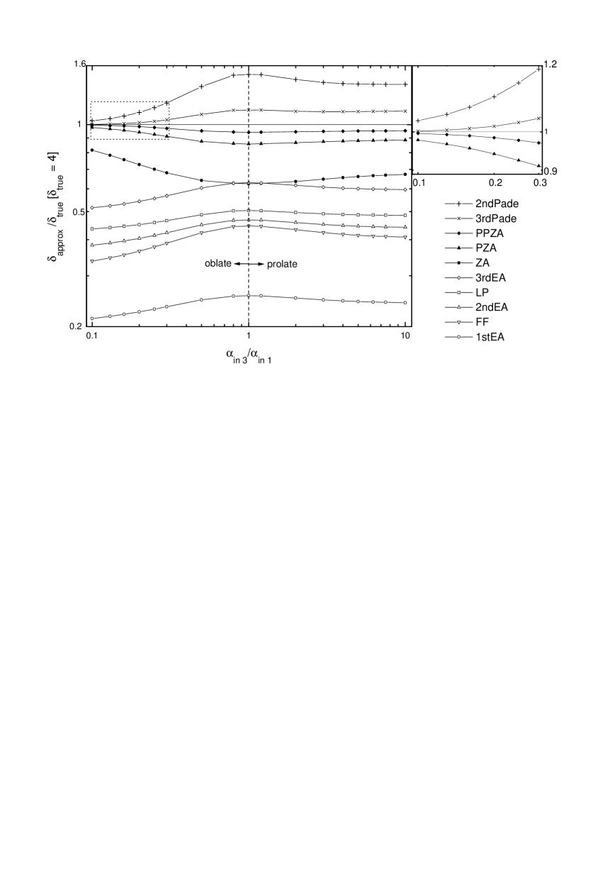
Figure 6: Density contrast of various approximations in spheroidal collapse of positive perturbations. This figure summarizes all the positive perturbations with various initial axis-ratios. The horizontal axis represents the initial axis-ratio $\alpha_{\rm in3}/\alpha_{\rm in1}$ and the vertical axis represents the ratio of density contrast $\delta_{\rm approx}/\delta_{\rm true}$ evaluated at $\delta_{\rm true}=4$.Both the axis ratio and density ratio are in logarithmic scale in this figure. The right square panel is the magnification of the part surrounded by the dotted line.

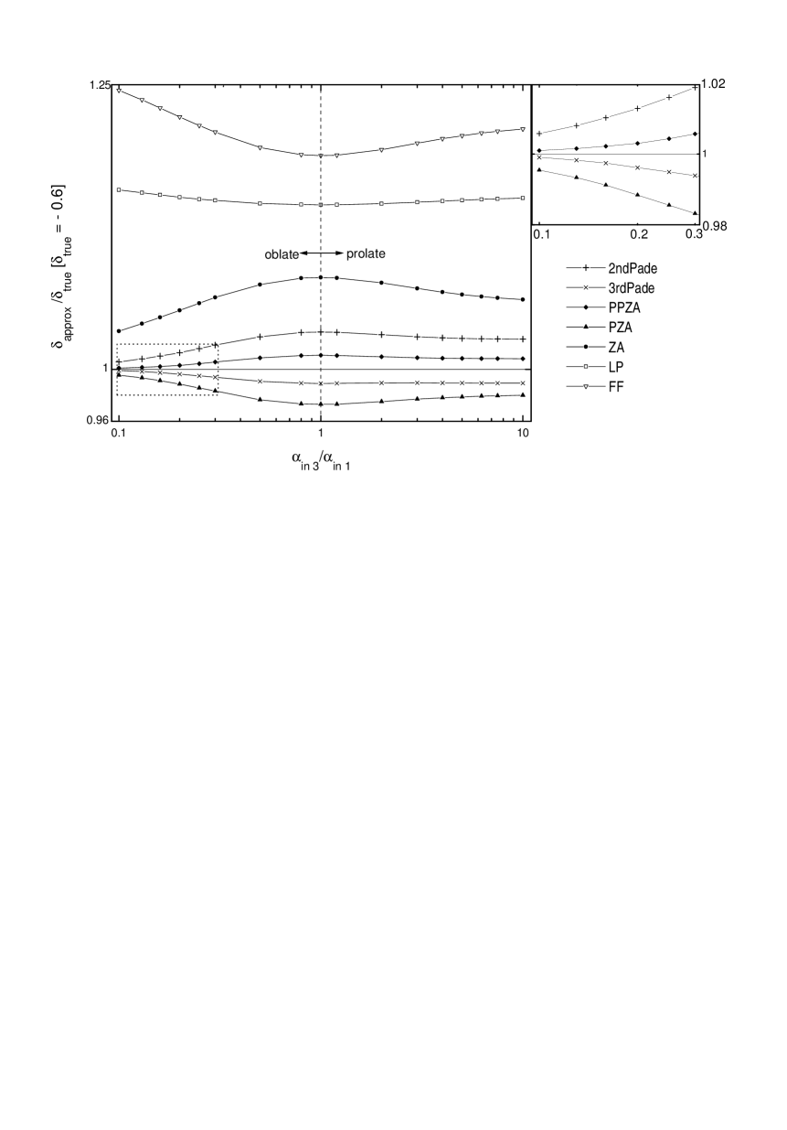
Figure 7: Density contrast of various approximations in spheroidal collapse of negative perturbations. This is the same as Fig. 6 but for negative perturbations. The horizontal axis represents the initial axis-ratio $\alpha_{\rm in3}/\alpha_{\rm in1}$ and the vertical axis represents the ratio of density contrast $\delta_{\rm approx}/\delta_{\rm true}$ evaluated at $\delta_{\rm true}=-0.6$. Both the axis ratio and density ratio are in logarithmic scale in this figure. The 1st $\sim$ 3rd Eulerian approximations are so bad that they are outside of this figure.

6 Conclusions and Discussions

In this paper, we have discussed the validity of the Zel’dovich-type approximations from the two aspects; (1) the dimensionality of the model and (2) the Lagrangian scheme on which the Zel’dovich-type approximations grounded. We introduced a model of spheroidal mass perturbations and compared several nonlinear approximations as well as Zel’dovich-type approximations.

We found the following facts from the spheroidal models. The accuracy of Zel’dovich-type approximations and Padé approximations becomes better in both prolate (effective dimension two) and oblate (effective dimension one) initial conditions compared with the spherical symmetric perturbations. Moreover the accuracy in oblate initial conditions is better than that in prolate initial conditions. These results may show that the Zel’dovich-type approximations are more accurate in lower dimensional collapse. All the other Eulerian approximations, on the other hand, have exactly the opposite tendency; the accuracy of them becomes worse in both prolate and oblate initial conditions. Moreover the accuracy in oblate initial conditions is worse than that in prolate initial conditions.

The above facts are consistent with the aspect (1) that the validity of the Zel’dovich-type approximations is due to the one-dimensional-exact property of them. On the other hand, the above facts conflict with the aspect (2) that the validity is grounded on the Lagrangian scheme of them. For the final confirmations of the aspect (1), we need further analysis on much wider class of models.

The last fact (vi) in the previous section suggests a possibility to construct a better approximation beyond Zel’dovich-type approximations by applying Padé method. Since Zel’dovich-type and Padé approximations are definitely different things, we may obtain new information when the Padé procedure is applied on the Zel’dovich-type approximations. The considerations on this possibility will be affirmatively reported in our separate publications.

For the actual analysis of observational quantities in the Universe, it is advantageous to use Eulerian scheme rather than Lagrangian scheme because the technique of classical field theory is most naturally applied in the former scheme. In this context, Padé approximations in Eulerian scheme, as they are accurate as Zel’dovich-type approximations, may open new perspective in the analysis of growth of density fluctuations in the expanding Universe. Of course we should keep in mind that the validity of the Padé approximation has not yet been fully established and therefore we should avoid blind applications of Padé method in cosmology.

We thank Masaaki Morita for helpful discussions on the dimensionality at the occasion of Tokyo Seminar at Mitaka National Observatory May 1997. We also thank Oki Nagahara for many suggestions in numerical calculations.

REFERENCES

Bagla, J. S., & Padmanabham, T. 1994, MNRAS, 266, 227

Bernardeau, F. 1994, ApJ, 427, 51

Bond, J. R., & Myers, S. T. 1996, ApJ, 103, 1

Brainerd, T. G., Scherrer, R. J., & Villumsen, J. V. 1993, ApJ, 418, 570

Binney, J., & Tremaine, S. 1987, Galactic Dynamics ( Princeton, NJ: Princeton Univ. Press)

Bouchet, F. R., Colombi, S., Hivon, E., & Juszkiewicz, R. 1995, A & A, 296, 575

Buchert, T. 1992, A & A, 223, 9

Buchert, T. 1994, MNRAS, 267, 811

Buchert, T., & Ehlers, J. 1993, MNRAS, 264, 375

Catelan, P. 1995, MNRAS, 276, 115

Eisenstein, D. J., & Loeb, A. 1995, ApJ, 439, 520

Fry, J. N. 1984, ApJ, 279, 499

Goroff, M. H., Grinstein, B., Rey S.-J., & Wise M. B. 1986, ApJ, 311, 6

Icke, V. 1973, A & A, 27, 1

Kellogg, O. 1953, Foundation of Potential Theory (New York: Dover)

Lin, C. C., Mestel, L., & Shu, F. H. 1965, ApJ, 142, 1431

Lynden-Bell, D. 1962, Proc. Cambridge Phil. Soc., 50, 709

Lynden-Bell, D. 1964, ApJ, 139, 1195

Matarrese, S., Lucchin, F., Moscardini, L., & Saez, D. 1992, MNRAS, 259, 437

Monaco, P. 1997, MNRAS, in press

Munshi, D., Sahni, V., & Starobinsky, A. A. 1994, ApJ, 436, 517

Peebles, P. J. E. 1980, The Large-Scale Structure of Universe ( Princeton, NJ: Princeton Univ. Press)

Press, W. H., Teukolsky, S. A., Vetterling, W. T., & Flannery, B. P. 1992, Numerical Recipes in Fortran ( 2nd ed.; Cambridge: Cambridge Univ. Press)

Sahni, V., & Coles, P. 1995, Phys. Rep., 262, 1

Sahni, V., & Shandarin, S. 1996, MNRAS, 282, 641

White, S. D. M., & Silk, J. 1979, ApJ, 231, 1

Zel’dovich, Ya. B. 1970, A & A, 5, 84

Zel’dovich, Ya. B. 1973, Astrophysics, 6, 164